© ESO, 2016

1. Introduction

It is well known that lags between gamma-ray burst (GRB) light curves observed in different spectral bands are a direct consequence of spectral evolution (Kocevski & Liang 2003; Schaefer 2004; Ryde 2005; Hakkila & Preece 2011). Obviously, with an invariant spectrum, all light curves would simply be proportional, therefore yielding zero lag. Lags provide an insight into the spectral evolution in GRBs from a temporal perspective. Moreover spectral lags have been found to correlate with burst luminosity and can be used as distance indicators (Norris et al. 2000; Norris 2002). In the present Swift and Fermi era more lags have been obtained in bursts with known distance, which allows the testing of the lag-luminosity relation with larger samples (Ukwatta et al. 2010, 2012; Bernardini et al. 2015; Heussaff 2015) or with better spectral coverage in individual events showing several pulses of different intensities (Zhang 2012; Shenoy et al. 2013).

Spectral evolution in GRBs generally goes from hard to soft within each pulse of the light curve. As a result, the pulse peaks earlier at high energy than at low energy, which corresponds (by definition) to a positive lag. Various mechanisms have been proposed to explain the spectral evolution, from a geometric origin resulting from the curvature of the emitting shells in the ejecta (Shen et al. 2005; Lu et al. 2006) to an intrinsic effect related to a true decrease of the peak energy with time (Kocevski & Liang 2003; Daigne & Mochkovitch 2003) or both (Peng et al. 2011).

To clarify the relationship between lags and spectral evolution Hafizi & Mochkovitch (2007) and Boçi et al. (2010) developed a simple analytical approach where the lag for a given pulse in the light curve is obtained from a linear expansion of the spectral parameters at pulse maximum. It appears from their result that the lag depends on the full spectral evolution, including E_p and the spectral indices α and β at low and high energy. In addition, the pulse shape and duration also affect the lag value for a given spectral evolution.

In the present work we use this approach to (i) analyse in some detail the lags measured with Fermi in the first pulse of the very bright burst GRB 130427A (Preece et al. 2014) and (ii) to statistically study a sample of lags obtained from the analysis of 70 Swift bursts (49 with known peak energy and luminosity). In Sect. 2 we present our analytical model and summarize its main results; the model is confronted with data in Sect. 3 and Sect. 4 is our conclusion.

2. A simple theory of lags

2.1. Analytical approach

The result obtained by Hafizi & Mochkovitch (2007) can be summarized by the following expression: $\mathit{\delta }{\mathit{t}}_{\mathrm{12}}\mathrm{=}\frac{{\mathit{f}}_{\mathrm{12}\mathit{,}{\mathit{E}}_{\mathrm{p}}}\hspace{0.17em}{\mathit{ė}}_{\mathrm{p}}\mathrm{+}{\mathit{f}}_{\mathrm{12}\mathit{,\alpha }}\hspace{0.17em}\mathit{ȧ}\mathrm{+}{\mathit{f}}_{\mathrm{12}\mathit{,\beta }}\hspace{0.17em}\mathit{ḃ}}{{\mathit{C}}_{\mathrm{1}}}\mathit{,}$(1)where the lag δt₁₂ between two energy bands 1[E_1,min,E_1,max] and 2[E_2,min,E_2,max] is defined as the difference in time between the pulse maxima in the two bands. This relation clearly establishes the link between lags and spectral evolution through the three quantities ė_p, ȧ, and ḃ, which are the logarithmic time derivatives of the peak energy E_p, and low and high energy spectral indices α and β, evaluated at pulse maximum t₁ in the low energy band 1. The three functions f_12,X in Eq. (1) are defined by${\mathit{f}}_{\mathrm{12}\mathit{,}\mathrm{X}}\mathrm{=}\frac{\mathit{\partial }\mathrm{Log}\hspace{0.17em}{\mathrm{ℱ}}_{\mathrm{12}}}{\mathit{\partial }\mathrm{Log}\hspace{0.17em}\mathit{X}}{|}_{{\mathit{t}}_{\mathrm{1}}}\mathit{,}$(2)where ${\mathrm{ℱ}}_{\mathrm{12}}\hspace{0.17em}\mathrm{\left(}{\mathit{E}}_{\mathrm{p}}\mathit{,\alpha ,\beta }\mathrm{\right)}\mathrm{=}\frac{{\mathrm{\int }}_{{\mathit{E}}_{\mathrm{2}\mathit{,}\min }\mathit{/}{\mathit{E}}_{\mathrm{p}}}^{{\mathit{E}}_{\mathrm{2}\mathit{,}\max }\mathit{/}{\mathit{E}}_{\mathrm{p}}}{\mathrm{ℬ}}_{\mathit{\alpha \beta }}\mathrm{\left(}\mathit{x}\mathrm{\right)}\hspace{0.17em}\mathrm{d}\mathit{x}}{{\mathrm{\int }}_{{\mathit{E}}_{\mathrm{1}\mathit{,}\min }\mathit{/}{\mathit{E}}_{\mathrm{p}}}^{{\mathit{E}}_{\mathrm{1}\mathit{,}\max }\mathit{/}{\mathit{E}}_{\mathrm{p}}}{\mathrm{ℬ}}_{\mathit{\alpha \beta }}\mathrm{\left(}\mathit{x}\mathrm{\right)}\hspace{0.17em}\mathrm{d}\mathit{x}}\mathit{,}$(3)and ℬ_αβ(x) is the spectral shape¹, which we approximate by a modified Band function $\mathrm{ℬ}\mathrm{\left(}\mathit{x}\mathrm{\right)}\mathrm{=}\{\begin{array}{c}\\ {\mathit{x}}^{\mathit{\alpha }}\hspace{0.17em}\exp \mathrm{[}\mathrm{-}\mathrm{(}\mathit{\alpha }\mathrm{+}\mathrm{2}\mathrm{)}{\frac{{\mathit{x}}^{\mathit{n}}}{\mathit{n}}}^{\mathrm{]}}\mathrm{for}\mathit{x}\mathrm{\le }{\mathit{x}}_{\mathrm{L}}\mathrm{=}{\mathrm{(}{\frac{\mathit{\alpha }\mathrm{-}\mathit{\beta }}{\mathit{\alpha }\mathrm{+}\mathrm{2}}}^{\mathrm{)}}}^{\mathrm{1}\mathit{/}\mathit{n}}\\ {\mathit{x}}^{\mathit{\beta }}\hspace{0.17em}{\mathit{x}}_{\mathrm{L}}^{\mathit{\alpha }\mathrm{-}\mathit{\beta }}\hspace{0.17em}\exp \hspace{0.17em}\mathrm{(}{\frac{\mathit{\beta }\mathrm{-}\mathit{\alpha }}{\mathit{n}}}^{\mathrm{)}}\mathrm{otherwise}\mathit{.}\end{array}$(4)The case with n = 1 represents the original Band function while n> 1 (resp. n< 1) corresponds to a narrower (resp. broader) transition between the two power laws as shown in Fig. 1, in which we represented x²ℬ(x) for n = 1, 2 and 0.67.

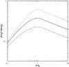Fig. 1 x2ℬ(x) spectra (with x = E/Ep) for α = −1, β = −2.3 and n = 1 in Eq. (4) (original Band function; full line), n = 2 (dotted line), and n = 0.67 (dashed line).

Finally, the C₁ parameter in Eq. (1) is the curvature of the pulse at time t₁${\mathit{C}}_{\mathrm{1}}\mathrm{=}\frac{{\begin{array}{c}\mathrm{¨}\\ \mathit{N}\end{array}}_{\mathrm{1}}\mathrm{\left(}{\mathit{t}}_{\mathrm{1}}\mathrm{\right)}}{{\mathit{N}}_{\mathrm{1}}\mathrm{\left(}{\mathit{t}}_{\mathrm{1}}\mathrm{\right)}}\mathit{,}$(5)where N₁(t) is the photon flux in band 1.

We can rewrite Eq. (1) in dimensionless form by introducing the pulse duration t_p, $\frac{\mathit{\delta }{\mathit{t}}_{\mathrm{12}}}{{\mathit{t}}_{\mathrm{p}}}\mathrm{=}\frac{{\mathit{f}}_{\mathrm{12}\mathit{,}{\mathit{E}}_{\mathrm{p}}}\hspace{0.17em}\mathit{\delta }{\mathit{e}}_{\mathrm{p}}\mathrm{+}{\mathit{f}}_{\mathrm{12}\mathit{,\alpha }}\hspace{0.17em}\mathit{\delta a}\mathrm{+}{\mathit{f}}_{\mathrm{12}\mathit{,\beta }}\hspace{0.17em}\mathit{\delta b}}{C_{\mathrm{1}}}\mathit{,}$(6)where δx = ẋ × t_p and $C_{\mathrm{1}}\mathrm{=}{\mathit{C}}_{\mathrm{1}}\mathrm{\times }{\mathit{t}}_{\mathrm{p}}^{\mathrm{2}}$. Equation (6) then shows that, for a given spectral evolution over the duration of the pulse (represented by the δx values), the lag is proportional to the pulse duration and inversely proportional to the “spikiness” C₁. Equation (6) therefore provides a simple explanation for the fact that short bursts generally have small lags.

2.2. Lags as a function of energy

2.2.1. Fixed E_p, different energy bands

We first consider a pulse with a Band spectrum of peak energy E_p, spectral indices, α and β, and temporal properties represented by the ratio t_p/C of the pulse duration to the curvature at pulse maximum (in a low energy band [10–20] keV). We compute the lag between this band and another band covering the interval [E–1.25E], where E is varied from 15 keV to 10 MeV. We adopt E_p = 500 keV, α = −1, β = −2.3, and t_p/ C = 0.3 s, and we consider three cases of spectral evolution with δe_p = −0.5 and δa = δb = 0, 0.1, and 0.2. The results are shown in Fig. 2a. The low energy band is always in the α part of the spectrum so that a change of behaviour takes place when the high energy band crosses E_p. The evolution of α (resp. β) mainly affects the lag below (resp. above) the break at E ≈ E_p. For a fixed spectral evolution, δe_p = −0.5 and δa = δb = 0.1, we also show in Fig. 2b the results for a modified Band spectrum with n = 2 and n = 0.67 in Eq. (4) and for the case of a power law with an exponential cut-off.

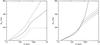Fig. 2 a)Left panel: lags between the low energy band [10–20] keV and a moving band [E-1.25E] as a function of E (in keV) for a pulse with tp/ C = 0.3 s and a Band spectrum (n = 1 in Eq. (4)) with Ep = 500 keV, α = −1, β = −2.3 for three different cases of spectral evolution: δep = −0.5 and δa = δb = 0 (dotted line), 0.1 (full line), and 0.2 (dashed line); b) right panel: same as a) for the case δep = −0.5 and δa = δb = 0.1 (full line), but also with a modified Band spectrum with n = 2 (dotted line) and n = 0.67 (dashed line). The full line with no break at 500 keV corresponds to a power-law spectrum with α = −1 and an exponential cut-off.

2.2.2. Fixed energy bands, different E_p

We now fix the two energy bands, 1 [100–150] keV and 2 [200–250] keV, which were used to obtain the lags in the source frame by Ukwatta et al. (2012), Bernardini et al. (2015), and Heussaff (2015), and in Fig. 3a we represent the lag as a function of the peak energy of the pulse spectrum. We first adopt a Band spectrum with α = −1, β = −2.3 and t_p/ C = 0.3 s and consider the same three cases of spectral evolution, δe_p = −0.5, δa = δb = 0, 0.1 and 0.2. As expected the lag is maximum when the peak energy lies just between the two bands, at about E_{p, ∗} = 175 keV. If the spectral evolution is limited to the peak energy (i.e. δa = δb = 0) the lag vanishes at low or high E_p values when the two energy bands are both in the same power-law part of the spectrum. Then the hardness ratio ℱ₁₂ (E_p,α,β) does not depend on E_p any more (see Eq. (3)) so that f_12,Ep = 0, leading to a zero lag if α and β do not evolve. Conversely, if the spectral evolution also affects the spectral indices (which is generally the case) the lag at low (resp. high) E_p is fixed by the evolution of β (resp. α). Then in Fig. 3b we show, for δe_p = −0.5, δa = δb = 0.1, the results for a modified Band spectrum with n = 2 or n = 0.67 and for a power law with an exponential cut-off. In this last case, the lag steadily rises at low E_p. This runaway feature however corresponds to the situation in which the flux in the high energy band shrinks owing to the exponential cut-off in the spectrum, which in practice would make the lag measurement very difficult.

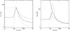Fig. 3 a)Left panel: lags between the two bands, [100–150] and [200–250] keV, as a function of the peak energy of the pulse spectrum. The spectral indices at low and high energy are α = −1 and β = −2.3. The curves correspond to the same three cases of spectral evolution considered in Fig. 2; b) right panel: same as a) for the case δep = −0.5 and δa = δb = 0.1 (full line), but also with a modified Band spectrum with n = 2 (dotted line) and n = 0.67 (dashed line). The full line that continuously rises at low Ep corresponds to a power-law spectrum with α = −1 and an exponential cut-off.

2.3. Comparison to a pulse model

To check the validity of the previous first order derivation of the spectral lag, we constructed a simple pulse model with a typical fast rise and an exponential decay luminosity profile 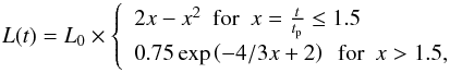$\mathit{L}\mathrm{\left(}\mathit{t}\mathrm{\right)}\mathrm{=}{\mathit{L}}_{\mathrm{0}}\mathrm{\times }\{\begin{array}{c}\\ \mathrm{2}\mathit{x}\mathrm{-}{\mathit{x}}^{\mathrm{2}}\mathrm{for}\mathit{x}\mathrm{=}\frac{\mathit{t}}{{\mathit{t}}_{\mathrm{p}}}\mathrm{\le }\mathrm{1.5}\\ \mathrm{0.75}\hspace{0.17em}\exp \mathrm{(}\mathrm{-}\mathrm{4}\mathit{/}\mathrm{3}\mathit{x}\mathrm{+}{\mathrm{2}}^{\mathrm{)}}\mathrm{for}\mathit{x}\mathit{>}\mathrm{1.5}\mathit{,}\end{array}$(7)so that the luminosity and its first derivative are continuous at x = 1.5 and where the spectral evolution takes the form 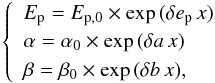$\{\begin{array}{c}\\ {\mathit{E}}_{\mathrm{p}}\mathrm{=}{\mathit{E}}_{\mathrm{p}\mathit{,}\mathrm{0}}\mathrm{\times }\exp \hspace{0.17em}\mathrm{\left(}\mathit{\delta }{\mathit{e}}_{\mathrm{p}}\hspace{0.17em}\mathit{x}\mathrm{\right)}\\ \mathit{\alpha }\mathrm{=}{\mathit{\alpha }}_{\mathrm{0}}\mathrm{\times }\exp \hspace{0.17em}\mathrm{\left(}\mathit{\delta a}\hspace{0.17em}\mathit{x}\mathrm{\right)}\\ \mathit{\beta }\mathrm{=}{\mathit{\beta }}_{\mathrm{0}}\mathrm{\times }\exp \hspace{0.17em}\mathrm{\left(}\mathit{\delta b}\hspace{0.17em}\mathit{x}\mathrm{\right)}\mathit{,}\end{array}$(8)where δe_p, δa, and δb have been defined in Eq. (6). From Eqs. (7) and (8) and assuming a Band spectrum (n = 1 in Eq. (4)), it is possible to compute the pulse profile in any spectral band. The results are shown in Fig. 4 for E_p,0 = 1000 keV, α₀ = −1, β₀ = −2.3, δe_p = −0.5, and δa = δb = 0.1, and the two bands 1 [10–20] and 2 [100–125] keV. The spectral lag δt₁₂ is calculated as the time difference between the pulse maxima at t_max,1 = 1.34 t_p and t_max,2 = 1.22 t_p, so that δt₁₂ = 0.12 t_p.

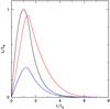Fig. 4 Light curves for the pulse model. The black curve shows the luminosity while the red and blue curves represent the photon flux in the [10–20] and [100–125] keV range, respectively. The flux unit is arbitrary, but the flux ratio between the two bands is respected.

We used this pulse model to check the analytical results. A comparison is shown in Fig. 5 for the lag-energy relation. As the analytical expression of the lag is obtained from a linear expansion around pulse maximum in the low energy band, we use in Eq. (6) the values of E_p, α, and β at t = t_max,1 = 1.34 s (i.e. assuming t_p = 1 s), which gives E_p = 512 keV, α = −1.14 and β = −2.63. The curvature is computed from the pulse model. We obtain | C₁ | = 3.1, which is somewhat larger than the curvature of the luminosity light curve | C_L | = 2, resulting from Eq. (7). It can be seen from Fig. 5 that the accuracy of the analytical expression is satisfactory, as the error does not exceed 20%, even at the large energy difference between the two spectral bands.

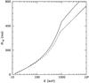Fig. 5 Lags between the low energy band [10–20] keV and a moving band [E–1.25E] as a function of E (in keV); comparison of the result from the pulse model (full line) and analytical expression (Eq. (1); dashed line).

2.4. The lag-luminosity relation

From the relation between the lag and peak energy at pulse maximum shown in Fig. 3, it is possible to obtain a lag-luminosity relation (LLR) if E_p is linked to the luminosity by a Yonetoku-like relation (Yonetoku et al. 2004) of the form ${\mathit{E}}_{\mathrm{p}}\mathrm{=}{\mathit{E}}_{\mathrm{0}}\hspace{0.17em}{\mathit{L}}_{\mathrm{52}}^{\mathit{ϵ}}\mathit{.}$(9)Adopting E₀ = 300 keV and ϵ = 0.5, we can directly transform Fig. 3a into the LLR shown in Fig. 6a. The LLR has two branches at low (L<L_∗) and high (L>L_∗) luminosity, where L_∗ ~ 3.4 × 10⁵¹ erg is the luminosity corresponding to E_p = E_{p, ∗} = 175 keV. If the spectral indices do not vary (δa = δb = 0), the lag in the low luminosity branch vanishes when the two considered spectral bands both lie above E_p. Then, the Band function simply reduces to a power law and f_12,Ep = 0. If δb ≠ 0, the lag takes the fixed value $\mathit{\delta }{\mathit{t}}_{\mathrm{12}}\mathrm{=}\frac{{\mathit{f}}_{\mathrm{12}\mathit{,\beta }}\hspace{0.17em}\mathit{\delta b}}{C_{\mathrm{1}}}\hspace{0.17em}{\mathit{t}}_{\mathrm{p}}\mathit{.}$(10)The situation is different when the spectrum is a power law with an exponential cut-off. In this case, the lag at low luminosity continuously increases. However (as already mentioned in Sect. 2.2.2 above) the flux in the high energy Band then becomes very low, making the lag measurement very difficult in practice.

In the high luminosity branch (i.e. at large E_p), the function f_12,Ep behaves as ${\mathit{E}}_{\mathrm{p}}^{-1}$ so that, if δa = 0, we get $\mathit{\delta }{\mathit{t}}_{\mathrm{12}}\mathrm{\propto }{\mathit{L}}^{\mathrm{-}\mathit{ϵ}}\mathit{.}$(11)If δa> 0 the LLR is steeper, becoming quasi-vertical when δa> 0.2. Finally, the variation of the LLR when the curvature of the spectrum is changed is shown in Fig. 6b for δe_p = −0.5, δa = δb = 0.1, and three values of n = 1, 0.67 and 2 in Eq. (4).

Fig. 6 a)Left panel: lag-luminosity relation for α = −1, β = −2.3, tp/ C = 0.3 s, δep = 0.5, and δa = δb = 0 (dotted line), 0.1 (full line), and 0.2 (dashed line). The full line that extends to large lag values at low luminosity corresponds to a power-law spectrum with α = −1 and an exponential cut-off; b) right panel: same as a) for the case δep = −0.5 and δa = δb = 0.1 (full line), but also with a modified Band spectrum with n = 2 (dotted line) and n = 0.67 (dashed line).

3. Comparison to observations

3.1. Lags of pulses and global lags

A potential problem in the comparison between data and model predictions comes from the fact that in the case of a complex burst, the measured lag is generally obtained by cross correlation of the light curves in the two considered spectral bands, while our model focuses on the lag of a single pulse, which is obtained as the time difference between the maxima in the two bands.

We first checked that for a single pulse this simple approach gives results that are close (within 10%) to those obtained by cross corelation. Then, in a complex burst with many pulses, where the global lag represents some average of the individual lags, we want to estimate the weight of each pulse in this average.

This can be carried out in a simple way when the pulses in the light curve do not overlap. Then for each pulse i the cross-correlation function of the profiles in two spectral bands 1 and 2 can be expanded around the maximum, ${\mathit{C}}_{\mathit{i}}\mathrm{\left(}\mathit{\delta t}\mathrm{\right)}\mathrm{\approx }{\mathit{C}}_{\mathit{i}}\mathrm{\left(}\mathit{\delta }{\mathit{t}}_{\mathrm{12}\mathit{,i}}\mathrm{\right)}\mathrm{-}{\mathit{N}}_{\mathrm{1}\mathit{,i}}{\mathit{N}}_{\mathrm{2}\mathit{,i}}\frac{\mathrm{(}\mathit{\delta t}\mathrm{-}\mathit{\delta }{\mathit{t}}_{\mathrm{12}\mathit{,i}}{\mathrm{)}}^{\mathrm{2}}}{\mathrm{2}{\mathit{t}}_{\mathrm{p}\mathit{,i}}}\hspace{0.17em}{C}_{\mathit{i}}\mathit{,}$(12)where N_1,i and N_2,i are the peak photon fluxes, δt_12,i is the spectral lag (for which C_i(δt) is maximum), t_p,i is the duration of the pulse, and C_i, a dimensionless measure of the pulse curvature (see Eq. (6)). The cross correlation for a profile with several well-separated pulses can be approximated by the sum of the individual functions, $\mathit{C}\mathrm{\left(}\mathit{\delta t}\mathrm{\right)}\mathrm{\approx }\sum _{\mathit{i}}{\mathit{C}}_{\mathit{i}}\mathrm{\left(}\mathit{\delta t}\mathrm{\right)}\mathit{.}$(13)The global lag δt₁₂ is then obtained by finding the maximum of C(δt), yielding 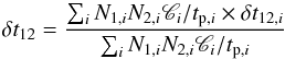$\mathit{\delta }{\mathit{t}}_{\mathrm{12}}\mathrm{=}\frac{{\sum }_{\mathit{i}}{\mathit{N}}_{\mathrm{1}\mathit{,i}}{\mathit{N}}_{\mathrm{2}\mathit{,i}}{C}_{\mathit{i}}\mathit{/}{\mathit{t}}_{\mathrm{p}\mathit{,i}}\mathrm{\times }\mathit{\delta }{\mathit{t}}_{\mathrm{12}\mathit{,i}}}{{\sum }_{\mathit{i}}{\mathit{N}}_{\mathrm{1}\mathit{,i}}{\mathit{N}}_{\mathrm{2}\mathit{,i}}{C}_{\mathit{i}}\mathit{/}{\mathit{t}}_{\mathrm{p}\mathit{,i}}}$(14)so that each individual lag appears in the average with a weight proportional to N_1,iN_2,iC_i/t_p,i. A bright, short or/and spiky pulse in a complex burst therefore imposes its lag on the whole event. In practice, the lag of brightest pulse generally dominates; see Hakkila et al. (2008). The global lag is averaged, however, in the case of several pulses with comparable weights, which can increase the dispersion of the LLR when it is generalized from individual pulses to the whole temporal history.

3.2. Detailed study of spectral lags in individual bursts: GRB 130427A

In some events, spectral lags have been obtained in several energy bands making possible a detailed comparison with the model and an estimate of the magnitude of spectral evolution. The best example is probably provided by the first pulse in GRB 130427A (Preece et al. 2014), where the high signal-to-noise ratio enabled a lag analysis from a few tens of keV to several MeV. Table 1 summarizes the results (transported in the burst rest frame). For the six lag value in Table 1 we also give the corresponding functions f_12,X that appear in Eq. (6)², where 1 represents the low energy band centred at 30 keV and 2 represents the high energy band (from 100 keV to 5 MeV). From Preece et al. (2014) we get the spectral parameters at pulse maximum in the low energy band (at t_obs = 0.5 s): E_p = 650 keV (rest frame), α = −0.57, and β = −3; the value β is not available for the first pulse and the adopted value corresponds to the whole event.

We then obtain estimates of the three quantities, x_e = δe_p/Q, x_a = δa/Q, and x_b = δb/Q, where Q = C₁/t_p, by minimizing the difference between the model results given by Eq. (6) and the observations $\mathrm{\Delta }\mathrm{=}\sum _{\mathrm{1}}^{\mathit{N}}\hspace{0.17em}{\left[\mathit{\delta }{\mathit{t}}_{\mathit{i}}\mathrm{-}\left({\mathit{f}}_{\mathrm{12}\mathit{,}{\mathrm{E}}_{\mathrm{p}}}^{\mathit{i}}\hspace{0.17em}{\mathit{x}}_{\mathit{e}}\mathrm{+}{\mathit{f}}_{\mathrm{12}\mathit{,\alpha }}^{\mathit{i}}\hspace{0.17em}{\mathit{x}}_{\mathit{a}}\mathrm{+}{\mathit{f}}_{\mathrm{12}\mathit{,\beta }}^{\mathit{i}}\hspace{0.17em}{\mathit{x}}_{\mathit{b}}\right)\right]}^{\hspace{0.17em}\mathrm{2}}\mathit{,}$(15)where the lags δt_i and the functions ${\mathit{f}}_{\mathrm{12}\mathit{,}\mathrm{X}}^{\mathit{i}}$ are given in Table 1. We began by considering only the first three lags (N = 3), which do not depend on β and its evolution since the high energy spectral band is still in the α part of the Band function. These lags also have values that are much smaller than the pulse duration, which allows us to use the linear approach of Eq. (6). We then included all six lag values (N = 6), which is more constraining but also possibly less accurate because the lag for the highest energy band is not much smaller than the pulse duration and the adopted high energy index β = −3 is just an average over the whole burst duration. In the first case, the resulting values are x_e = 0.087 and x_a = −0.065 (x_b is not constrained), while in the second we obtain x_e = 0.06, x_a = −0.08 and x_b = −0.025, showing a difference of 35% in x_e and of 20% in x_a. These values are then used to obtain the lag-energy relation, which is shown for the two cases in Fig. 7 together with the data points.

The time-resolved spectral analysis available for the first pulse partially allows us to test the consistency of the results. At pulse maximum one finds from the data that δe_p ≃ −1 and δa ≃ 0.6. Then with t_p = 0.5 s / (1 + z) ≈ 0.37 s (rest-frame value), we get ${\mathit{x}}_{\mathit{e}}\mathrm{\simeq }\mathrm{-}\mathrm{0.09}{}^{\mathrm{\right(}}\frac{\mathrm{4}}{C_{\mathrm{1}}}^{\mathrm{\left)}}$ and ${\mathit{x}}_{\mathit{a}}\mathrm{\simeq }\mathrm{0.055}{}^{\mathrm{\right(}}\frac{\mathrm{4}}{C_{\mathrm{1}}}^{\mathrm{\left)}}$. With C₁ = 4, which seems reasonable even if a highly accurate measure of the curvature is difficult, the results obtained from the first three lags are in very good agreement with the observed spectral evolution. When all six lag values are included in the analysis, the agreement is less satisfactory, probably from the combined effects of using Eq. (6) out of its domain of validity and the uncertainty in β.

3.3. Monte Carlo approach to the observed lag-luminosity relation

Ukwatta et al. (2012), Bernardini et al. (2015), and Heussaff (2015) recently constructed samples of rest-frame lags for long bursts with known redshift observed with the Swift satellite. From the 49 (of 70) long GRBs in the Heussaff (2015) sample (see Table 2), which have a measured peak energy and luminosity, 20 have a positive lag while the error bars for the others only allow us to fix an upper limit to the lag (in one case, this upper limit is negative). For comparison with our analytical results, we developed a simple Monte Carlo approach, in which the spectral and temporal parameters of the generated events are drawn according to the following distributions³:

• The low energy spectral index α has a normal distribution centred at α = −1 with a standard deviation σ_α = 0.25 (Kaneko et al. 2006).

• The high energy spectral index β has a truncated normal distribution centred at β = −2.3 with the same standard deviation but truncated to exclude all values of β> −2 (Kaneko et al. 2006).

• The pulse duration also follows a log-normal distribution with ⟨Log t_p⟩ = 0 and σ_Logtp = 0.35 (Nakar & Piran 2002).

• The peak energy follows a log-normal distribution with ⟨Log E_p⟩ = 2.7 (rest frame) and σ_LogEp = 0.25 (Kaneko et al. 2006; Ghirlanda et al. 2012).

• The luminosity is obtained from the peak energy using the Yonetoku relation (Eq. (9)) where we added a dispersion of 0.5 in Log L.

The parameters controlling the spectral evolution, δe_p, δa, and δb, and the spikiness C, are weakly constrained. We first fix their values to δe_p = −0.5, δa = δb = 0, 0.1, or 0.2 and | C| = 3.33 (so that ⟨t_p⟩ / | C | ≃ 0.3 . We then draw the burst parameters according to the above rules and get the corresponding lag using Eq. (6). The slope of the resulting LLR strongly depends on the adopted value for δa, going from −2.4 for δa = 0 to −5 for δa = 0.1 and −7.5 for δa = 0.2. These slopes (especially for δa ≠ 0) appear too steep when compared to the data. One possible way to solve this discrepancy is to introduce some kind of variability-luminosity relation of the form 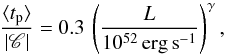$\frac{\mathrm{⟨}{\mathit{t}}_{\mathrm{p}}\mathrm{⟩}}{\mathrm{\left|}C\mathrm{\right|}}\mathrm{=}\mathrm{0.3}\hspace{0.17em}{\left(\frac{\mathit{L}}{{\mathrm{10}}^{\mathrm{52}}\hspace{0.17em}{\mathrm{erg}\hspace{0.17em}\mathrm{s}}^{-1}}\right)}^{\mathit{\gamma }}\mathit{,}$(16)with γ ~ 0.1–0.2, i.e. corresponding to a situation where the pulses become narrower or/and spikier as their luminosity increases. A few observational studies have suggested these relations (Reichart et al. 2001; Hakkila et al. 2008), but they would clearly need further confirmation. Adopting γ = 0.15, the three slopes are reduced to −0.4, −2.6, and −3.1 for δa = 0, 0.1 and 0.2, respectively. The case with δa = 0.1 is shown in Fig. 8, where we represented the LLR together with the cumulative and differential distribution of lags. These lags are compared to the data from Heussaff (2015). It can be seen that the main difference comes from observed bursts with negative lags that are not produced by the simulation.

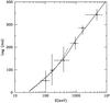Fig. 7 Lags as a function of energy in GRB 130427A. The six measured values (Preece et al. 2014) are fitted using our model with Ep = 650 keV, α = −0.57, β = −3 and xe = 0.061, xa = −0.08, xb = −0.025 (full line) and xe = 0.087, xa = 0.065 (dashed line); see text for details.

If we suppose that these negative lags result from measurement uncertainties and can be ignored, the model fits the data well. Conversely, if the existence of negative lags is confirmed (see Chen et al. 2005; Roychoudhury et al. 2014 for details) one simple way to produce them would be to suppose that the time derivative of the low energy spectral index α at pulse maximum can be positive (i.e. δa negative in Eq. (6) corresponding to a soft to hard evolution for α). For example, adopting for δa a normal distribution centred at 0 with a dispersion of 0.15, 15% of the lags are negative. The corresponding LLR and distribution of lags are shown in Fig. 9 (the negative lags do not appear in the LLR owing to the logarithmic scale) showing an excellent agreement with the data; a KS test indicates that the difference of 0.157 between the observed and predicted cumulative distribution functions has a probability of 17% of happening from random fluctuations.

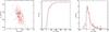Fig. 8 Lag-luminosity relation, cumulative, and differential distributions of lags for δep = 0.5, δa = δb = 0.1, and ⟨tp⟩ / |C | given by Eq. (15) with γ = 0.15; left panel: 250 simulated events (red circles) and data points from Heussaff (2015; black dots); middle panel: cumulative distribution of lags; right panel: differential distribution of lags. In the middle and right panels the observed distribution is binned in interval of 10 ms.

Fig. 9 Same as Fig. 8 but δa now has a normal distribution with ⟨δa⟩ = 0 and a dispersion of 0.15.

The above results were obtained with a Band spectrum (n = 1 in Eq. (4)) but we checked how they are modified when we adopt (i) a power law with an exponential cut-off or (ii) a value of n different from unity. In the first case, the effect is moderate since, for a majority of the simulated spectra, the two considered spectral bands lie below E_p whose central value is 500 keV (rest frame) in our simulation. In the second case, we tested the value n = 2, corresponding to an increased curvature at the peak. It allows us to obtain the same slopes for the LLR with γ = 0.05 only, i.e. practically without supposing the variability-luminosity relation of Eq. (15).

4. Conclusions

Based on our previous work (Hafizi & Mochkovitch 2007; Boçi et al. 2010), we compared the results from a simple analytical expression of the spectral lags in GRBs to data collected by the Swift and Fermi satellites. This expression (Eq. (6)) explicitly connects the lag of a pulse in the light curve to its spectral (E_p, α, β, and their time derivatives) and temporal (pulse duration and curvature at the peak) parameters. We checked the accuracy of the analytical expression with a pulse model. It proved to be accurate within 20% even when the two considered spectral bands are wide apart. For the two bands [100–150] and [200–250] keV, we obtained the lag as a function of the peak energy of the spectrum (Fig. 3). Then, assuming a Yonetoku-like relation between the peak energy at pulse maximum and the luminosity, we derived a theoretical LLR (Fig. 6). When the spectral evolution is limited to variations of the peak energy (α and β staying constant) the lag is given by a power law, δt ∝ L^{− ϵ} at high luminosity, where ϵ is the exponent of the Yonetoku-like relation E_p ∝ L^ϵ. If the spectral indices also vary (from hard to soft within a pulse), the LLR becomes steeper than L^ϵ.

We first tested the relation between lags and energy using Fermi data for the first pulse in the light curve of GRB 130427A. The fit of six lag values allows us to constrain the evolution of both E_p and the spectral indices, and the consistency of the results can be tested with the time-resolved spectral analysis available for this event. We then used a Monte Carlo approach where the spectral and temporal parameters were drawn according to the observed distributions and the results were compared to the lag analysis of 49 Swift bursts with known peak energy and luminosity performed by Heussaff (2015). The synthetic LLR appears steeper than the observed LLR, which can be corrected if the duration t_p or/and curvature C of the pulses are correlated to the luminosity. We presented results with a moderate correlation ⟨t_p⟩ / | C | ∝ L^0.15, which are in good agreement with the data except for the fact that the synthetic distribution does not show any negative lag contrary to the observed distribution. If these negative lags are real, a simple way to produce them in the model would be to allow the low energy spectral index to evolve from soft to hard in some cases.

Both the observational and model LLRs show that the lags globally decrease with increasing luminosity. However the correlation is rather steep and has a large dispersion, which probably prevents from using lags as an accurate distance indicator. In Fig. 8, with fixed values of δe_p, δa, and δb, the typical luminosity interval for a given lag typically spans one order of magnitude already. With a dispersion added for δa (Fig. 9, left panel) this interval rises to 1.5 orders of magnitude. At low luminosity (below 10⁵¹ erg s^-1, where very limited data is available) a variety of behaviours are possible, as shown in Fig. 6. If the spectrum is a genuine or modified Band function, the lag vanishes if the high energy spectral index does not vary or takes a fixed value in the opposite (more realistic) case. If the spectrum is a power law with an exponential cut-off, the lag continuously increases but the low flux in the high energy band makes it difficult to measure in practice.

The comparison between our model and the data relied on a collection bursts mostly observed by Swift. As a result of the

limited spectral coverage of the BAT instrument, the interval between the spectral bands used to obtain the lags is reduced, which results in small lag values that are easily affected by uncertainties. With Fermi and the future Chinese-French SVOM mission (Cordier et al. 2015) better lag estimates can and will be obtained using more separated spectral bands that will better constrain the spectral evolution, as illustrated here in the case of GRB 130427. In addition, SVOM will be able to provide the lags and the reshift simultaneously, which will allow for better testing of the LLR and its value as a distance indicator.

Acknowledgments

It is a pleasure to thank Frédéric Daigne for helpful discussions and the anonymous referee for valuable comments, which helped to improve the manuscript.

References

All Tables

All Figures

	Fig. 1 x2ℬ(x) spectra (with x = E/Ep) for α = −1, β = −2.3 and n = 1 in Eq. (4) (original Band function; full line), n = 2 (dotted line), and n = 0.67 (dashed line).
In the text

Fig. 2 a)Left panel: lags between the low energy band [10–20] keV and a moving band [E-1.25E] as a function of E (in keV) for a pulse with tp/ C = 0.3 s and a Band spectrum (n = 1 in Eq. (4)) with Ep = 500 keV, α = −1, β = −2.3 for three different cases of spectral evolution: δep = −0.5 and δa = δb = 0 (dotted line), 0.1 (full line), and 0.2 (dashed line); b) right panel: same as a) for the case δep = −0.5 and δa = δb = 0.1 (full line), but also with a modified Band spectrum with n = 2 (dotted line) and n = 0.67 (dashed line). The full line with no break at 500 keV corresponds to a power-law spectrum with α = −1 and an exponential cut-off.

In the text

Fig. 3 a)Left panel: lags between the two bands, [100–150] and [200–250] keV, as a function of the peak energy of the pulse spectrum. The spectral indices at low and high energy are α = −1 and β = −2.3. The curves correspond to the same three cases of spectral evolution considered in Fig. 2; b) right panel: same as a) for the case δep = −0.5 and δa = δb = 0.1 (full line), but also with a modified Band spectrum with n = 2 (dotted line) and n = 0.67 (dashed line). The full line that continuously rises at low Ep corresponds to a power-law spectrum with α = −1 and an exponential cut-off.

In the text

	Fig. 4 Light curves for the pulse model. The black curve shows the luminosity while the red and blue curves represent the photon flux in the [10–20] and [100–125] keV range, respectively. The flux unit is arbitrary, but the flux ratio between the two bands is respected.
In the text

	Fig. 5 Lags between the low energy band [10–20] keV and a moving band [E–1.25E] as a function of E (in keV); comparison of the result from the pulse model (full line) and analytical expression (Eq. (1); dashed line).
In the text

Fig. 6 a)Left panel: lag-luminosity relation for α = −1, β = −2.3, tp/ C = 0.3 s, δep = 0.5, and δa = δb = 0 (dotted line), 0.1 (full line), and 0.2 (dashed line). The full line that extends to large lag values at low luminosity corresponds to a power-law spectrum with α = −1 and an exponential cut-off; b) right panel: same as a) for the case δep = −0.5 and δa = δb = 0.1 (full line), but also with a modified Band spectrum with n = 2 (dotted line) and n = 0.67 (dashed line).

In the text

	Fig. 7 Lags as a function of energy in GRB 130427A. The six measured values (Preece et al. 2014) are fitted using our model with Ep = 650 keV, α = −0.57, β = −3 and xe = 0.061, xa = −0.08, xb = −0.025 (full line) and xe = 0.087, xa = 0.065 (dashed line); see text for details.
In the text

Fig. 8 Lag-luminosity relation, cumulative, and differential distributions of lags for δep = 0.5, δa = δb = 0.1, and ⟨tp⟩ / |C | given by Eq. (15) with γ = 0.15; left panel: 250 simulated events (red circles) and data points from Heussaff (2015; black dots); middle panel: cumulative distribution of lags; right panel: differential distribution of lags. In the middle and right panels the observed distribution is binned in interval of 10 ms.

In the text

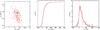	Fig. 9 Same as Fig. 8 but δa now has a normal distribution with ⟨δa⟩ = 0 and a dispersion of 0.15.
In the text

References

- Bernardini, M. G., Ghirlanda, G., Campana, S., et al. 2015, MNRAS, 446, 1129 [NASA ADS] [CrossRef] [Google Scholar]
- Boçi, S., Hafizi, M., & Mochkovitch, R. 2010, A&A, 519, A76 [NASA ADS] [CrossRef] [EDP Sciences] [Google Scholar]
- Chen, L., Lou, Y.-Q., Wu, M., et al. 2005, ApJ, 619, 983 [NASA ADS] [CrossRef] [Google Scholar]
- Cordier, B., Wei, J., Atteia, J.-L., et al. 2015, ArXiv e-prints [arXiv:1512.03323] [Google Scholar]
- Daigne, F., & Mochkovitch, R. 2003, MNRAS, 342, 587 [NASA ADS] [CrossRef] [Google Scholar]
- Ghirlanda, G., Nava, L., Ghisellini, G., et al. 2012, MNRAS, 420, 483 [NASA ADS] [CrossRef] [Google Scholar]
- Hafizi, M., & Mochkovitch, R. 2007, A&A, 465, 67 [NASA ADS] [CrossRef] [EDP Sciences] [Google Scholar]
- Hakkila, J., & Preece, R. D. 2011, ApJ, 740, 104 [NASA ADS] [CrossRef] [Google Scholar]
- Hakkila, J., Giblin, T. W., Norris, J. P., Fragile, P. C., & Bonnell, J. T. 2008, ApJ, 677, L81 [NASA ADS] [CrossRef] [Google Scholar]
- Heussaff, V. 2015, Ph.D. Thesis, Université Toulouse III, Paul Sabatier [Google Scholar]
- Kaneko, Y., Preece, R. D., Briggs, M. S., et al. 2006, ApJS, 166, 298 [NASA ADS] [CrossRef] [Google Scholar]
- Kocevski, D., & Liang, E. 2003, ApJ, 594, 385 [NASA ADS] [CrossRef] [Google Scholar]
- Lu, R.-J., Qin, Y.-P., Zhang, Z.-B., & Yi, T.-F. 2006, MNRAS, 367, 275 [NASA ADS] [CrossRef] [Google Scholar]
- Nakar, E., & Piran, T. 2002, MNRAS, 331, 40 [NASA ADS] [CrossRef] [Google Scholar]
- Norris, J. P. 2002, ApJ, 579, 386 [NASA ADS] [CrossRef] [Google Scholar]
- Norris, J. P., Marani, G. F., & Bonnell, J. T. 2000, ApJ, 534, 248 [NASA ADS] [CrossRef] [Google Scholar]
- Peng, Z. Y., Yin, Y., Bi, X. W., Bao, Y. Y., & Ma, L. 2011, Astron. Nachr., 332, 92 [NASA ADS] [CrossRef] [Google Scholar]
- Preece, R., Burgess, J. M., von Kienlin, A., et al. 2014, Science, 343, 51 [NASA ADS] [CrossRef] [Google Scholar]
- Reichart, D. E., Lamb, D. Q., Fenimore, E. E., et al. 2001, ApJ, 552, 57 [NASA ADS] [CrossRef] [Google Scholar]
- Roychoudhury, A., Sarkar, S. K., & Bhadra, A. 2014, ApJ, 782, 105 [NASA ADS] [CrossRef] [Google Scholar]
- Ryde, F. 2005, A&A, 429, 869 [NASA ADS] [CrossRef] [EDP Sciences] [Google Scholar]
- Schaefer, B. E. 2004, ApJ, 602, 306 [NASA ADS] [CrossRef] [Google Scholar]
- Shen, R.-F., Song, L.-M., & Li, Z. 2005, MNRAS, 362, 59 [NASA ADS] [CrossRef] [Google Scholar]
- Shenoy, A., Sonbas, E., Dermer, C., et al. 2013, ApJ, 778, 3 [NASA ADS] [CrossRef] [Google Scholar]
- Ukwatta, T. N., Stamatikos, M., Dhuga, K. S., et al. 2010, ApJ, 711, 1073 [NASA ADS] [CrossRef] [Google Scholar]
- Ukwatta, T. N., Dhuga, K. S., Stamatikos, M., et al. 2012, MNRAS, 419, 614 [NASA ADS] [CrossRef] [Google Scholar]
- Yonetoku, D., Murakami, T., Nakamura, T., et al. 2004, ApJ, 609, 935 [NASA ADS] [CrossRef] [Google Scholar]
- Zhang, F.-W. 2012, Ap&SS, 339, 123 [NASA ADS] [CrossRef] [Google Scholar]
All Tables
Spectral lags (in burst rest frame) between a low energy band centred at 30 keV and six other spectral bands for the first pulse in GRB 130427A; the corresponding functions f12,X evaluated at pulse maximum in the low energy band are also given.
The 49 bursts with redshift and measured peak energy and luminosity in Heussaff (2015).