| Issue |
A&A
Volume 592, August 2016
|
|
|---|---|---|
| Article Number | A62 | |
| Number of page(s) | 12 | |
| Section | Numerical methods and codes | |
| DOI | https://doi.org/10.1051/0004-6361/201527143 | |
| Published online | 25 July 2016 | |
Comparison of black hole growth in galaxy mergers with gasoline and ramses
1 CEA-Saclay, IRFU, SAp, 91191 Gif-sur-Yvette, France
e-mail: This email address is being protected from spambots. You need JavaScript enabled to view it.
2 Institut d’Astrophysique de Paris,
UMR 7095 CNRS, Université Pierre et Marie Curie, 98bis Bd Arago, 75014
Paris,
France
3 Center for Theoretical Astrophysics
and Cosmology, Institute for Computational Science, University of Zurich,
Winterthurerstrasse
190, 8057
Zurich,
Switzerland
4 Department of Astrophysics,
American Museum of Natural History,
Central Park West at 79th Street, New York, NY
10024,
USA
5 Astronomy Department, University of
Washington, Box
351580, Seattle,
WA
98195-1580,
USA
Received:
8
August
2015
Accepted:
22
April
2016
Abstract
Supermassive black hole dynamics during galaxy mergers is crucial in determining the rate of black hole mergers and cosmic black hole growth. As simulations achieve higher resolution, it becomes important to assess whether the black hole dynamics is influenced by the treatment of the interstellar medium in different simulation codes. We compare simulations of black hole growth in galaxy mergers with two codes: the smoothed particle hydrodynamics code gasoline, and the adaptive mesh refinement code ramses. We seek to identify predictions of these models that are robust despite differences in hydrodynamic methods and implementations of subgrid physics. We find that the general behavior is consistent between codes. Black hole accretion is minimal while the galaxies are well-separated (and even as they fly by within 10 kpc at the first pericenter). At late stages, when the galaxies pass within a few kpc, tidal torques drive nuclear gas inflow that triggers bursts of black hole accretion accompanied by star formation. We also note quantitative discrepancies that are model dependent: our ramses simulations show less star formation and black hole growth, and a smoother gas distribution with larger clumps and filaments than our gasoline simulations. We attribute these differences primarily to the subgrid models for black hole fueling, feedback, and gas thermodynamics. The main conclusion is that differences exist quantitatively between codes, and this should be kept in mind when making comparisons with observations. However, both codes capture the same dynamical behaviors in terms of triggering black hole accretion, star formation, and black hole dynamics, which is reassuring.
Key words: galaxies: active / galaxies: evolution / galaxies: formation / galaxies: interactions / galaxies: star formation
© ESO 2016
1. Introduction
Galaxy mergers are thought to be transformational events in galaxy evolution. Mergers transform stellar disks into spheroids (e.g., Toomre & Toomre 1972; Gerhard 1981; Negroponte & White 1983; Barnes & Hernquist 1996). Via tidal torques, they tend to compress gas into the central regions of galaxies, triggering powerful starbursts (e.g., Sanders et al. 1988; Barnes & Hernquist 1991; Mihos & Hernquist 1996). The increase in nuclear gas is also thought to fuel growth in galaxies’ central supermassive black holes, resulting in active galactic nuclei (AGNs, e.g., Sanders et al. 1988; Hernquist 1989; Di Matteo et al. 2005).
Correlations between supermassive black hole mass and global galaxy properties (see Kormendy & Ho 2013, and references therein) suggest a possible evolutionary link between black holes and galaxy growth (e.g., Silk & Rees 1998; Wyithe & Loeb 2003). The energetic output from AGNs may provide a physical driver for this link; in some cases, they emit sufficient energy to heat up all the cold gas in a galaxy, and they may trigger powerful outflows (e.g., Crenshaw et al. 2003; Di Matteo et al. 2005; Rupke & Veilleux 2011; Gabor & Bournaud 2014). Active galactic nuclei sometimes power radio jets that can heat intergalactic and intracluster gas (e.g., Fabian et al. 2000; Voit & Donahue 2005; Randall et al. 2011). AGNs have been invoked in many models of galaxy evolution as a primary actor in regulating the star formation rates (SFRs) and stellar masses of the most massive galaxies (e.g., Hopkins et al. 2006; Croton et al. 2006; Somerville et al. 2008).
Numerical hydrodynamic simulations have led to many advances in our understanding of galaxy mergers and black hole fueling, but we have not yet developed a complete understanding of how the results depend on the details of these models. Different studies have used various treatments of hydrodynamics and feedback processes (such as supernova and AGN output), as well as different resolution. Details of the feedback treatment can have an important effect on black hole growth and its impact on galaxies (e.g., Debuhr et al. 2011; Wurster & Thacker 2013b,a; Newton & Kay 2013).
Differences in hydrodynamic method can also lead to differences in simulated galaxy (and intergalactic) properties in various contexts. Recent work shows that smoothed particle hydrodynamics (SPH; Lucy 1977; Gingold & Monaghan 1977), historically a commonly used method in extragalactic astrophysics for solving the equations of hydrodynamics, is inaccurate in certain circumstances, for example in resolving shocks and in Kelvin-Helmholtz and Rayleigh-Taylor instabilities (Agertz et al. 2007). Grid techniques such as adaptive mesh refinement (AMR; Berger & Colella 1989) generally improve these problems (Agertz et al. 2007), but with drawbacks including advection errors, angular momentum conservation, and numerical diffusion (e.g., Wadsley et al. 2008; Hahn et al. 2010; see discussion and references in Hopkins 2014). More recent hybrid techniques employing a moving mesh (Springel 2010) or no mesh at all (Hopkins 2014) can help resolve these difficulties.
In cosmological simulations, traditional SPH as implemented in the gadget code (Springel 2005) tends to allow a smaller quantity of gas to cool and to fuel galaxies than mesh-based codes, leading to smaller gas disks (Kereš et al. 2012; Vogelsberger et al. 2012; Scannapieco et al. 2012). The apparently suppressed cooling in SPH relative to moving mesh methods also allows the formation of more prominent hot halos in idealized merger simulations, along with clumps and filaments in those halos (Hayward et al. 2014). This is true even though – in cosmological SPH simulations – a smaller proportion of gas accreting onto galaxies passes through a hot phase (Nelson et al. 2013)1. Despite these important differences, it appears that differences in feedback implementations cause more prominent changes than differences in the numerical method for hydrodynamics (Scannapieco et al. 2012). Moving forward, large code-comparison projects like AGORA (Kim et al. 2014) should help clarify these issues in the context of galaxy evolution. With the exception of Hayward et al. (2014), the impact of different codes and numerical techniques on supermassive black hole fueling and feedback has not been studied.
In this work, we compare high-resolution simulations of black hole growth in galaxy mergers with two codes, the gasoline SPH code and the ramses AMR code. While many authors have used SPH codes to study black holes in idealized galaxy mergers, relatively few have used AMR codes (see, e.g., Kim et al. 2011). We use standard physical recipes in both codes for star formation, black hole growth, and stellar and black hole feedback. In Sect. 2 we describe the simulations. Then we highlight similarities and differences, and attempt to explain them, in Sect. 3. We conclude in Sect. 4.
2. Simulations
For our analysis, we focus on four representative simulations of galaxy mergers, two run with gasoline and two with ramses. The merging galaxies have mass ratios of 2:1 and 4:1, gas fractions of 30%, and disks oriented coplanar with their orbits. We also ran some resolution tests and simulations with other mass ratios and orbital configurations (see Capelo et al. 2015), which give similar results. In this paper we focus on the 4:1 merger simulation as a representative case. Below we give the numerical details of the gasoline simulations and include details of the initial conditions, and then we describe the ramses simulations.
2.1. Methods: GASOLINE
We use a subset of the suite of gasoline merger simulations described fully in Capelo et al. (2015). We summarize the simulations here. gasoline (Wadsley et al. 2004), an N-body SPH code, is based on pkdgrav (Stadel 2001), which uses a tree method to calculate gravitational dynamics among particles. We note that these simulations do not include recent improvements in the SPH method (Keller et al. 2014). As a Lagrangian particle code, the resolution is automatically adaptive; the highest resolution occurs in the densest regions.
gasoline includes models for gas cooling, star formation, supernovae and stellar winds, and black hole accretion and feedback. The simulations use a standard model for gas cooling, which incorporates metal cooling (Shen et al. 2010). A temperature floor of 500 K is imposed.
Star formation occurs as a random process (see Katz 1992) in gas particles colder than 6000 K and denser than 100 H atoms cm-3. The SFR is calculated by assuming that a fraction ϵ∗ = 1.5% of the eligible gas forms into stars per star formation time, where the star formation time is the greater of the gas free fall time or the gas cooling time. With a probability consistent with the star formation rate and timestep, a star-forming gas particle will convert some of its mass into a collisionless star particle.
Stellar feedback includes a blast wave model for Type II supernovae (SNe; all model details are given in Stinson et al. 2006). The stellar population represented by a star particle is assumed to have an initial mass function from Miller & Scalo (1979), which determines the number of SN-progenitor stars above 8 M⊙. These stars will explode at the ends of their lifetimes, which depend on the mass of the star (and metallicity) according to the model of Raiteri et al. (1996). In a given simulation timestep, supernova energy is calculated based on the mass of young stars that should explode during that time, and 1051 erg per SN is distributed (along with gas mass and metals) among gas particles that are neighbors of the star particle. To mimic an expanding blast wave, gas cooling is turned off for a time that depends on the local gas conditions and the feedback energy. This cooling delay time, based on the SN remnant survival time from the model of McKee & Ostriker (1977), is given by Eq. (11) of Stinson et al. (2006):  yr. Here, E51 is the SN energy in units of 1051 ergs, n0 is the ambient hydrogen density in cm-3, kB is Boltzmann’s constant, and P04 is 10-4 times the ambient gas pressure.
Nuclear black holes are treated as sink particles that accrete surrounding gas (Bellovary et al. 2010). The accretion rate onto the black hole is calculated separately for each neighboring gas particle based on a Bondi accretion rate (see Bondi 1952), and the sum of the rates from each gas particle yields the total accretion rate. Mass is then removed from the gas particles in proportion to their contribution to the accretion rate, and the mass is added to the black hole. We note that the Bondi accretion rate here includes a small boost factor α2 (see Booth & Schaye 2009 for a discussion of boost factors). The accretion rate is capped at α times the Eddington Limit. A fixed fraction ϵr = 0.1 of the accreted mass-energy is emitted as radiation at each timestep, and a coupling fraction ϵf = 0.001 of the radiated energy injected as thermal energy into the nearest gas particle. These parameter values are taken from the literature and are calibrated so that the remnants of simulated galaxy mergers match the observed local MBH − Mbulge relation (Van Wassenhove et al. 2014).
2.1.1. gasoline simulation setup and initial conditions
We set up mergers of two disk galaxies as in Capelo et al. (2015). Galaxies begin with parabolic orbits (Benson 2005), have initial separations that are the sum of the two galaxies’ virial radii, and have a separation at the first pericenter equal to 20% of the virial radius of the larger galaxy (Khochfar & Burkert 2006). The galactic disks are coplanar with their orbits, and both galaxies rotate in the same direction as the orbit (prograde-prograde mergers).
Each model galaxy includes five components: a dark matter halo, a stellar bulge, a stellar disk, a gaseous disk, and a supermassive black hole (Springel & White 1999; Springel et al. 2005). The dark matter halo follows a Navarro et al. (1996) profile up to the virial radius, with an exponential decay beyond. It has spin parameter λ = 0.04 and concentration c = 3. The stellar bulge makes up 0.8% of the virial mass, and follows a Hernquist (1990) profile. The galactic disk makes up 4% of the virial mass, and follows an exponential surface density profile. The disk scale radius is derived from conservation of angular momentum of the material making up the disk. Thirty percent of the disk mass is gas, so that the fraction of total baryons in gas (the common observational definition of gas fraction) is 0.3(0.04Mvir)/(0.04Mvir + 0.008Mvir) = 0.25. Supermassive black holes with masses 2 × 10⁻³ times the bulge mass (Marconi & Hunt 2003) are placed at the centers of initialized galaxies. In each simulation, the primary galaxy has a virial mass of 2.21 × 10¹¹M⊙, bulge mass 1.77 × 10⁹M⊙, disk mass 8.83 × 10⁹M⊙, and disk scale radius of 1.13 kpc. The secondary galaxies have their masses scaled down by factors of two and four, respectively.
Dark matter particles, initial star particles, and initial gas particles have masses of 1.1 × 10⁵M⊙, 3.3 × 10³M⊙, and 4.6 × 10³M⊙, respectively, with softening lengths of 30 pc, 10 pc, and 20 pc. At the beginning of the simulation, the 1:2 merger includes 4 913 826 dark matter particles, 3 840 163 star particles, and 836 883 gas particles (the primary galaxy alone contains two-thirds of these numbers). The 1:4 merger includes 4 094 855 dark matter particles, 3 201 816 star particles, and 696 605 gas particles.
Model galaxies undergo a relaxation period of 100 Myr in isolation before they begin the merger. During this period, the star formation efficiency ϵ∗ is gradually increased to its final value, 1.5%, to prevent unphysical bursts of supernova feedback. After this relaxation, the supermassive black hole masses are reset to their initial values, and the galaxies are placed in appropriate orbits for the mergers.
2.2. Methods: RAMSES
We ran a small new suite of merger simulations using the ramses AMR code (Teyssier 2002). Our setup borrows many aspects from Gabor & Bournaud (2013, 2014) and Perret et al. (2014), and mostly uses standard recipes for physical processes. ramses solves the equations of hydrodynamics on the mesh, while it treats collisionless matter (dark matter and stars) as particles. The effects of gravity are calculated on the mesh using a multigrid method, and particle accelerations are interpolated using a cloud-in-cell method.
We use the standard quasi-Lagrangian mesh refinement criteria: a cell is refined if it contains more than 30 dark matter particles or if the mass in the cell exceeds 5 × 10³M⊙. In addition, we refine cells whose mass is sufficiently large that the local gas Jeans length is not resolved by at least 4 cell widths (Truelove et al. 1997). These refinement criteria ensure that the highest resolution is applied to the densest regions, where star-forming clouds form.
The thermodynamics is treated with a standard model for gas cooling, including metal cooling (e.g., Teyssier et al. 2013). We impose an overall temperature floor of 100 K, as well as a density-dependent temperature floor (the Jeans polytrope) that ensures the local Jeans length in the smallest grid cells is always resolved by at least 4 cells (Machacek et al. 2001). The Jeans polytrope acts as an additional pressure (or pressure floor) that prevents numerical fragmentation. The normalization of this temperature floor depends on resolution, and is higher for lower resolution simulations.
ramses includes models for star formation and supernova feedback. Star formation occurs as a random process in cells whose gas density (or particle number) exceeds 100 H atoms cm-3. In cells above this threshold density, a fraction ϵ∗ = 1 percent of the gas is assumed to form into stars per free fall time, yielding an SFR for each cell. A new collisionless star particle is created in the cell with a probability based on the SFR and the timestep. New star particles inherit the position and velocity of the gas cell out of which they formed, but they are decoupled and will generally move into other cells.
After a delay of 10 Myr, supernovae explode at the locations of newly formed star particles. Twenty percent of the mass of the initial star particle is assumed to explode as supernovae, and for each 10 M⊙ of exploding supernova, 1051 erg of thermal energy is added to the hosting cell. Following Stinson et al. (2006) and Teyssier et al. (2013), cooling is delayed for 20 Myr in the supernova-heated cell to enable more efficient feedback.
Supermassive black holes are represented by collisionless sink particles. The sink particles accrete gas according to a Bondi accretion rate (see Bondi 1952), where the gas density and temperature are computed from a weighted average of all gas cells within 4Δx (where Δx is the smallest cell size, Krumholz et al. 2004). We use the standard Bondi formula, without a “boost” factor α (Booth & Schaye 2009). The accretion rate is capped at the Eddington limit, assuming a radiative efficiency ϵr = 0.1. Black hole particles merge once they pass within 4Δx of one another.
Black hole feedback is implemented as a thermal deposition of energy (Dubois et al. 2010; Teyssier et al. 2011). A fraction ϵr = 0.1 of the accreted mass is assumed to convert into radiative energy, and a fraction ϵc = 0.15 of the radiative energy is assumed to couple with the surrounding gas as thermal heating (Booth & Schaye 2009; Dubois et al. 2010; Teyssier et al. 2011). These AGN model parameters have been calibrated in cosmological simulations to yield an MBH − Mbulge relation that matches observations (Dubois et al. 2012). Following Booth & Schaye (2009), we only inject AGN feedback energy if it is sufficient to heat the surrounding gas to Tmin,AGN = 107 K. This prevents the deposited energy from being immediately radiatively cooled from dense gas, leading to more efficient feedback. On timesteps where the feedback energy is insufficient to heat the gas to Tmin,AGN, we store the feedback energy to be added to that during the following timesteps. This storage is repeated until enough energy is stored to reach Tmin,AGN, at which time it is released. We deposit the feedback energy in gas cells within 4Δx with a weighting where colder, denser gas acquires more of the energy (Gabor & Bournaud 2013). If the post-injection gas temperature exceeds Tmax,AGN = 5 × 10⁹ K, then we iteratively expand the injection radius by 25 percent to dilute the injection energy and lower the injection temperature. This maximum injection temperature prevents the extremely high temperatures that can cause computational problems (Gabor & Bournaud 2013).
As noted in Gabor & Bournaud (2013), numerous tests show that black holes sometimes scatter from the centers of their host galaxies by hundreds of pc. In merger simulations, the scattering is even more pronounced. Some of this scattering is a numerical artifact; it essentially does not occur in the gasoline simulations (except on small scales, which can be reduced with improved dynamical friction modeling; see Tremmel et al. 2015). The scattering in ramses is reduced, but not eliminated, when a more accurate direct-summation N-body gravity solver is applied to the sink particle (see Bleuler & Teyssier 2014). On the other hand, some scattering at the ~102 pc level is physically realistic given the dynamics in the nucleus: in ramses, gas clumps may form with masses ~10 times the mass of the black hole, so a close encounter can displace the black hole from the galaxy center. These events are rare, with more typical scattering at the level of tens of pc. To limit black hole scattering, we adopt a well-known solution of assigning a black hole dynamical mass that is much larger than the true mass (e.g., Debuhr et al. 2010). For the gravity calculation, the black hole is assigned a mass of 109M⊙, while we use the true mass for black-hole-specific physics (e.g., Bondi accretion). This effectively keeps the black holes in their galactic centers by increasing the dynamical friction due to stars and dark matter. We will sometimes refer to these black holes as artificially massive.
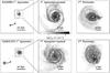 |
Fig. 1 Snapshots showing gas surface density for our 4:1 ramses (top) and gasoline (bottom) simulations. Left panels show both galaxies at first apocenter, with arrows roughly indicating the direction of travel of the secondary galaxy. Middle panels show a zoom-in on the primary galaxy at first apocenter, and right panels show both galaxies at the second pericenter. In the right panels, circles mark the positions of the black holes (in each simulation, the more massive black hole is to the left). |
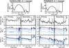 |
Fig. 2 BH separation in kpc (top), black hole accretion rate (BHAR) in M⊙ yr-1 (second row), gas mass in M⊙ within spheres up to 1 kpc in radius (third row), and SFR in M⊙ yr-1 within the same spheres (bottom row) vs. time for a 4:1 merger with gasoline (left) and ramses (right). For each simulation, we show quantities for the primary galaxy/BH on the left, and the secondary galaxy/BH on the right. We show gas masses and SFRs within radii of 200 pc to 1 kpc, in increments of 200 pc. Quantities are smoothed on 10 Myr timescales. Note that time-axes differ by ~20% (see Sect. 3.2.1). Vertical dotted lines mark local minima in the separation between the two black holes in all panels. The gasoline and ramses simulations show qualitatively similar results: enhanced accretion and star formation rates at the second pericenter, and especially at the third pericenter/coalescence. |
2.2.1. ramses simulation setup and initial conditions
Initial conditions for the ramses simulations are generated separately from those for the gasoline runs, following the description in Gabor & Bournaud (2013). We use the same masses, density profiles and numbers of particles (for stars and for dark matter) as in the gasoline simulations, and initialize the positions and velocity distributions with the Cartesian grid code from Bournaud & Combes (2002).
The initial conditions generator determines equilibrium positions and phase-space velocity distributions for stellar and dark matter particles, taking into account the gas disk contribution to the gravitational potential, and the gas density distribution if initialized analytically in ramses. We also must initialize gas cells outside the disk: technically, null densities could not be handled properly. We do this by setting their density very low (~10-7 cm-3) so that the initial contribution to the circum-galactic halo is marginal: this halo will form from outflows during the simulation. Supermassive black holes are added to the galactic centers at the start of the ramses runs.
A necessary difference with the gasoline initial conditions is that the dark matter halo must be truncated to fit within the chosen simulation box size. While SPH simulations do not require a box size, AMR simulations do in order to set up the initial grid. Choosing an arbitrarily large box size would incur substantial computational costs; calculations must be done on – and memory must be used to store information about – grid cells that are far away from the galaxies and have little impact on the results. Although we chose a box size of 250 kpc for the ramses runs to include a large majority of the mass, the gasoline halos include mass extending beyond 150 kpc in radius from each galaxy center.
We set up the ramses initial conditions in boxes of width 130 kpc (roughly half the width of the full simulation box since the merging galaxies are initially separated). In order to fit the halos within the box, we truncate them more aggressively than in the gasoline case; after relaxation, the outer parts of ramses halos have an exponential decline with a characteristic radius half that of the gasoline halos. To maintain the halo truncation over time, we also truncated the Maxwellian distribution of velocities for dark matter particles at 90% of the local escape velocity (computed at the initial position of each particle), otherwise the halo expands spatially over time and dynamically evaporates from the ramses simulation box. When truncating the halos, we made the choice to keep the same total halo mass, so at very large separations during the early phases of the interaction the two galaxies have the same total masses and keep similar orbits with the two codes, and undergo their collision under nearly identical configurations. At lower separations, however, once the systems start to overlap the halo densities start to differ: halos generated this way end up with slightly higher masses within R200 and smaller radii than the gasoline halos (by ≲10 percent), so short-range gravity and dynamical friction are somewhat stronger in the ramses simulations. This will be discussed later when comparing the detailed evolution of each merging system.
As in the gasoline case, we want each galaxy to undergo a relaxation period of ~100 Myr. We do not have a simple method for inserting a fully relaxed galaxy into a ramses merger simulation, so the relaxation must occur during the main simulation. Given our orbital parameters, the galaxies remain quasi-isolated and undisturbed by tidal forces during the first 200−300 Myr of the merger, which is sufficient to allow relaxation (1–2 disk dynamical times) and allow the formation of internal features such as bars and spiral arms before the interaction itself occurs. During this relaxation phase we restrict refinement up to level 11 (spatial resolution ≈120 pc), but allow star formation. The relatively poor resolution helps restrict formation of dense gas clouds, so star formation proceeds slowly, forming a total of a few ×108M⊙ stars during the first 200 Myr (representing ~10% of the initial gas mass, compared to nearly 20 % for the gasoline case).
For the merger, galaxies begin with the same orbital parameters (initial separation and velocities) and orientations (prograde-prograde) as in the gasoline simulations. The mergers evolve in a cubic box with a size of 250 kpc. We use a base grid level of 6, corresponding to cells with a size of ≈3900 pc, and we allow refinement up to level 15, corresponding to a minimum cell size of about 7.6 pc.
3. Results
3.1. General behavior: common features
Figure 1 presents face-on images of gas surface density in our 4:1 ramses and gasoline simulations. In each image pixel, we calculate the gas surface density by summing all the gas mass falling within the pixel along the line of sight through the entire simulation box and then dividing by the pixel area. For ramses, this entails summing the gas in all gas cells along the line of sight that fall in the pixel, with appropriate corrections for partial overlap of cells with the pixel. For gasoline, this entails integrating the overlapping portion of the SPH smoothing kernel for every gas particle within one projected smoothing length of the pixel. First we show the first apocenter, then a zoom-in of the primary galaxy at the same snapshot, and finally the merging galaxies at the second pericenter.
In Fig. 2 we compare the time evolution of various quantities during a 4:1 merger in our gasoline and ramses simulations. At the top, we show the separation between the primary and secondary black holes. Below the separation plots, separately for the primary and secondary, we show the black hole accretion rates (BHARs), gas masses within 1 kpc of the black hole, and SFRs within 1 kpc of the black hole. For the last two, we show the gas mass within spheres of five different radii, equally spaced from 200 pc to 1000 pc. Careful comparison of the ramses and gasoline snapshots in Fig. 1 and in the top panels of Fig. 2 indicates some differences in the galaxy orbits (e.g., in ramses the galaxies are farther apart at first apocenter), and differences in gas structures (e.g., in gasoline gas forms into smaller clouds). We will address these differences in Sect. 3.2.
Overall, however, the dynamics of the black holes is similar until we can follow them in a consistent way. We note here that in our gasoline simulations the black holes never merge, whereas in ramses they merge when the galaxies coalesce, shortly after the third pericenter, once they pass within each other’s accretion radii (in this case about 60 pc). Black hole mergers are implemented in gasoline, but we chose to turn them off to study the dynamical behavior (Van Wassenhove et al. 2014; Capelo et al. 2015). This choice affects accretion on the black holes, and therefore we refrain from commenting on black hole growth at late times in the simulation.
The patterns in star formation and black hole accretion driven by dynamics, i.e., how merger-driven inflows at pericenters enhance them, are also similar once the differences in the orbits are taken into account. Indeed, one of the main conclusions of our experiment is that even when trying to make the simulation setups (i.e. initial conditions and implementations of star formation and BH growth) as similar as possible to each other, the way parameters are set up is intrinsically different, and therefore differences arise even in a controlled experiment.
Qualitatively, the behavior in gasoline and ramses simulations is similar. At the first pericenter, the black holes pass within about 10 kpc of each other, but this induces little gas inflow and little change in the BHARs or SFRs. Between the first and second pericenters, the galaxies act as though they are isolated with relatively steady SFRs and BHARs. During this time the SFRs and especially the BHARs fluctuate on short timescales; in the BHAR case, fluctuations of an order of magnitude are common. These fluctuations result from stochastic fueling of the central black hole (Hopkins & Hernquist 2006), driven both by structure in the interstellar medium (ISM) and by AGN feedback (Gabor & Bournaud 2013). Following Capelo et al. (2015), we call this the stochastic phase of the merger.
The action begins at the second pericenter. As the two black holes pass within a few kpc, tidal torques trigger an increase in gas mass within the central few hundred pc in both the primary and secondary galaxies. The increase in central gas mass, which is more pronounced in the secondary, triggers enhanced central star formation and black hole growth. At the third pericenter ~150 Myr later, the interaction induces another burst of activity. In both simulations, this picture (starting at the second pericenter) roughly follows the well-known scenario of merger-driven starburst and AGN fueling (Sanders et al. 1988; Barnes & Hernquist 1991; Di Matteo et al. 2005).
In summary, the overall behavior of the ramses and gasoline simulations is similar, and broadly consistent with previous studies of galaxy mergers. There are, however, important discrepancies between the two simulations, which we address next. Understanding these differences and why they arise is important in order to extract and retain the results that we can consider robust.
3.2. Quantitative discrepancies
3.2.1. Orbits
The galaxy orbits differ slightly between the gasoline and ramses runs, as implied by the top panels of Fig. 2. In the gasoline run, the galaxies move to wider separations between the first and second pericentric passages (around t = 500 Myr), and the second pericenter occurs at a later time (~1.0 Gyr rather than ~0.8 Gyr in the ramses case). Since the mergers are initialized with the same positions and velocities in both simulations, we attribute these differences to mass discrepancies.
As described in Sect. 2, galaxy halos in ramses simulations must be truncated to fit inside a computationally reasonable box size. When we created the initial conditions, we chose to keep the total halo mass constant, so the truncation increases the dark matter density by a few percent inside the truncation radius. If instead we had kept the central density constant, then the total halo mass would be modified and the interaction orbit would start to differ even at large separations before the two galaxies overlap or develop tidal features. Instead, our choice keeps the early-stage configuration of the interaction relatively unchanged (as suggested by the nearly identical first pericenter times in the upper panels of Fig. 2). Subsequently, the higher central density of the truncated ramses halo increases the gravitational forces at shorter distances once the two halos start to significantly overlap. We attribute the faster merging in ramses to this difference rather than to effects of the codes themselves (e.g., Poisson solver type or accuracy). To further probe this, we analytically estimated the timescale required to “free-fall” from the first apocenter to the next encounter at ≤5 kpc, assuming the radial profile of the halos and baryonic components did not evolve from the initial conditions: the timescales are 382 Myr for the gasoline initial mass distribution, and 327 Myr for ramses. The timescales measured in the simulations are about 350 and 290 Myr, respectively; they are both shorter than our analytic estimates (probably owing to the extra effects of dynamical friction and/or increased mass concentration at the first pericenter), but the relative difference of ≃15% is fully consistent with that in the analytical estimate. Hence, the faster merging timescale in the ramses merger results from our choice of keeping the total halo mass constant when a truncation is applied to the initial conditions.
3.2.2. Black hole accretion rates
During the relatively quiescent phase between the first and second pericenter, the BHARs differ significanly in the two simulations (see Fig. 2): ramses BHARs fluctuate around 10-4.5M⊙ yr-1, while those in gasoline fluctuate around 10-3.5M⊙ yr-1. In any case, the black hole growth during this period is small because the accretion rates are low. Thus the detailed level of black hole fueling is relatively unimportant during the quiescent phase.
During the merger phase, the primary BHs show marked differences in the BHAR. In gasoline, the primary BHAR peaks sharply (by a factor >10) just after the second pericenter, remains elevated (with large fluctuations) until the third pericenter, and rises again just after the third pericenter. In ramses, the primary shows a brief spike in BHAR at the second pericenter, then returns to the quiescent level even through the third pericenter, until experiencing another spike at coalescence. The secondary BHARs, in contrast, are similar in both simulations, showing a peak in BHAR at the second pericenter and another peak at the third pericenter that lasts through coalescence. In ramses, black hole coalescence occurs ~50 Myr after the third pericenter, whereas coalescence never occurs in gasoline. The coalescence limits dual black hole growth in the merger remnant.
We attribute these quantitative discrepancies in black hole growth between gasoline and ramses mainly to differences in the black hole fueling and feedback models. In gasoline, the accretion rate includes a small boost factor to the formal Bondi rate (typically α = 3; see Sect. 2.1), and the feedback coupling efficiency is set to a relatively low value of 0.1% (calibrated from idealized merger simulations Van Wassenhove et al. 2014). Thermal energy from feedback is dumped into a single nearby particle at every timestep without any storage. In ramses, on the other hand, the accretion rate includes no boost factor, and the coupling efficiency is set to a relatively high value of 0.15 (calibrated from cosmological simulations with much lower resolution and slightly different feedback prescriptions; see Booth & Schaye 2009; Dubois et al. 2012). Feedback energy is dumped into the entire accretion region, but only if enough energy is “stored” to heat the gas in that region to 107 K, which increases the effective efficiency.
Black hole growth is mostly self-regulated in these simulations, suggesting that the difference in coupling efficiency causes more of a difference than the boost factor. The efficient feedback in ramses keeps the gas immediately around the black hole hot and diffuse, leading to lower accretion rates than in gasoline. This effect persists throughout both the stochastic phase and merger phase. Owing to the efficient feedback, bursts of accretion in ramses (see Fig. 2) are short-lived and they drive only minor BH growth.
The implementation of supernova (SN) feedback in this set of ramses simulations may also contribute to suppressing black hole growth. Dubois et al. (2015) find that when the SN feedback implementation in ramses includes delayed cooling, black hole growth is suppressed in galaxies with bulge mass below ~109M⊙, which is comparable to the bulge mass in our runs.
This BH growth discrepancy raises questions about the choice of AGN feedback efficiency. Our best method of calibrating the efficiency relies on comparing simulated black hole growth to observed BH demographics and MBH-galaxy relations, especially MBH − Mbulge. This was done using large-scale cosmological simulations for ramses, and idealized mergers and zoomed simulations for gasoline (Bellovary et al. 2013). Combined with the discrepancies in BH growth, this suggests that the optimal efficiency could depend on resolution and stellar feedback effects. If so, this calibration could be especially problematic when pushing the boundaries of simulation resolution; it is computationally expensive to run several high-resolution simulations just for calibration.
In summary, different physical prescriptions for black hole fueling and feedback dominate over differences in hydrodynamic method (see Hayward et al. 2014). The efficient AGN feedback in ramses leads to lower BH accretion rates than in gasoline. The Mgas plots in Fig. 2 – which show less gas inflow at late stages in ramses than in gasoline – suggest that gas dynamics play a role as well. In the next sections, we explore how the models for gas thermodynamics influence the gas structure of the galaxies, which in turn will influence the details of gas dynamics.
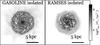 |
Fig. 3 Face-on images of gas surface density of an isolated disk galaxy simulation using gasoline (left) and ramses (right). The characteristic sizes of gas structures are larger in ramses than in gasoline due partly to the Jeans polytrope pressure floor implemented in ramses and partly to differences in more fundamental aspects of the codes (e.g., hydrodynamic or gravity solvers). |
3.2.3. Galaxy gas structure
Figure 1 (especially the middle panels) suggests a key difference in gas structure between our ramses and gasoline simulations: gas forms larger, smoother structures in ramses. In order to eliminate any possible effects of the galaxy merger, we compare these same primary galaxies but in an isolated context. We show images from these in Fig. 3. As in Fig. 1, we show projected gas surface density, computed in the same way as described in Sect. 3.1.
In the case of gasoline, we show a snapshot at 200 Myr of the 4:1 merger. This is well before the first pericenter, and thus the galaxy appears as it would in isolation. For the ramses case, we recall that the galaxies do not undergo a separate relaxation simulation before beginning the merger simulation, as the gasoline galaxies do. Thus the galaxies relax during the first 200–300 Myr before the first pericenter. In order to make a fair comparison with the isolated gasoline galaxy, we ran a separate ramses simulation with an isolated version of the primary galaxy. We show a snapshot from this isolated ramses simulation at about 250 Myr, which is similar to the age of the gasoline galaxy.
Figure 3 reinforces the difference in gas structure. In ramses the gas forms thick filaments and large clumps, whereas in gasoline the gas forms many smaller filaments and clouds with a more flocculent appearance. Moreover, dense gas structures appear to extend to larger radii in gasoline, while the ramses outer disk is quite smooth.
To quantify the differences in gas structure, we calculate the power spectrum of 2D spatial variations (as in Christensen et al. 2012). We first crop each gas surface density map shown in Fig. 3 to a width of L ≈ 6 kpc to isolate the galaxy ISM, then calculate the 2D fast Fourier transform. This yields a 2D image in frequency space,  , where u and v are frequency coordinates. We shift the image so that zero frequency is at the image center, and calculate the 2D power as
  . From the 2D power image we calculate the 1D power spectrum, P(k), by calculating the average power per pixel in a concentric set of circular annuli. Here, k refers to the radius in pixels of each annulus placed on the frequency-space image; k is a spatial frequency coordinate related to spatial wavelength λ via λ = L/k. Structures of size s correspond to a wavelength of λ = 2s. Finally, we normalize the power spectrum by a power law to clarify the differences between simulations: in Fig. 4 we show P′(s) = P(s)/(0.024s3). A third-degree power law roughly fits the shape of P(s), so this normalization flattens the trend.
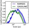 |
Fig. 4 Power spectra of gas surface density fluctuations in isolated gasoline and ramses galaxies. The power spectra are normalized by a third-degree power law to highlight the differences between simulations. Shaded error regions indicate the 10–90th percentile range from bootstrap resampling. gasoline shows more power at small scales and less power at large scales, emphasizing that gas structures in our gasoline simulations tend to have smaller sizes than those in ramses. |
We also calculate spatial variations in the power spectrum using a bootstrapping technique, and we show them as error regions in Fig. 4. First we divide the 2D power image into 20 wedges centered on the image center, each subtending an angle of 360/20 = 18 deg. Then we create a bootstrap replicate image by randomly selecting among wedges (with replacement), rotating each wedge to fill one of the 20 positions, and joining the rotated wedges together into a single image. We create 500 such bootstrap replicate images. We measure the 1D power spectrum on each image (as above), so that for each spatial frequency we have a distribution of 500 bootstrap power spectrum values. We show the 10th and 90th percentiles of this distribution as our error regions. This bootstrap technique yields very similar results to calculating the standard errors in each annulus when measuring the 1D power spectrum on the original image. The width between the 10th and 90th percentiles shown is marginally larger than the 1σ standard errors.
Figure 4 shows that our gasoline simulation has more power than ramses on scales s smaller than ≈100 pc, and less power on scales larger than ~200 pc. This confirms that the sizes of gas structures in gasoline indeed tend to be smaller than those in ramses. Both simulations have the same amount of power on scales ~100–200 pc, which is approximately the width of filaments and clumps in the ramses simulation (i.e., the Jeans length). The gasoline simulation includes structures of this size, but their internal fragmentation leads to the enhanced power on smaller scales.
In the following section, we argue that the relative excess of gas structure on large scales in ramses is due to the implementation of a Jeans polytrope, the pressure floor that stabilizes the gas (which is absent from the gasoline simulations).
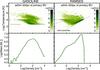 |
Fig. 5 Density-temperature diagrams (top row) and density PDFs (bottom row) for gas in gasoline (left column) and ramses (right column). We show only gas within 500 pc of the primary galactic center in each simulation, and we use a snapshot near the maximum separation (first apocenter, around 500 Myr). In the top panels, we include the temperature distribution along the left axis (arbitrarily normalized and shown on a linear scale). We also schematically show the Jeans polytrope temperature floor for the ramses simulation (straight black line), which keeps the average gas significantly hotter than in gasoline. |
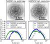 |
Fig. 6 Gas surface density maps (top) and power spectra (bottom) for ramses simulations of isolated galaxies with different settings: Left: simulation with no Jeans polytrope pressure floor. Right: simulation with a more easily triggered refinement criterion that enables ≈15 pc resolution throughout the galactic disk (and without the Jeans polytrope). Removing the Jeans polytrope ensures that the power on scales ≳200 pc is similar in ramses and gasoline simulations. Enhancing the typical cell size in ramses leads to improved agreement between ramses and gasoline power spectra on scales ≲50 pc at the expense of a discrepancy at moderate scales of ≈50–200 pc (as well as additional computational cost). |
3.2.4. Stabilization by the Jeans polytrope
In Fig. 5, we show density-temperature diagrams and density distributions in both gasoline and ramses. We show only gas within 500 pc of the primary BH at a timestep during the stochastic phase, between the first and second pericenters. This gas is representative of gas in the disk of the galaxy.
We also schematically show the Jeans polytrope in the ramses density-temperature diagram. By construction, gas in ramses is not allowed to fall below this line. In contrast, a significant amount of gas in gasoline exists at lower temperatures and higher densities than imposed by this floor in ramses. At the gasoline temperature floor of 500 K, gas at the threshold for star formation (100 cm-3) is resolved by ≈64 gas particles (with poorer relative resolution with increasing gas density). We note that gasoline includes an option to use a Jeans polytrope, but it frequently goes unused in galaxy formation simulations (as here) mainly because the cold dense gas to which it applies is always star-forming gas, which is treated with a subgrid star formation model.
The thermal pressure imposed by the effective density-dependent temperature floor in ramses helps stabilize the galaxy’s gas disk against gravitational collapse. Gas does not reach densities higher than about 103 cm-3, whereas the high-density tail in gasoline, where the temperature floor is independent of density, reaches 104 cm-3 (bottom panels of Fig. 5). The gas temperature distribution (along the left axis of the density-temperature diagram) in ramses has a broad peak around 104 K, while in gasoline it shows a bimodal structure: a small peak around 104 K, and a larger peak around 500 K (the temperature floor). In both simulations a substantial portion of the gas reaches the temperature floor, but in ramses the temperature floor is set by the Jeans polytrope.
The higher typical gas temperature in ramses implies a more pressurized ISM, and a larger Jeans length (and Jeans mass). The larger Jeans length naturally leads to larger collapsed structures, giving rise to the larger filaments and gas clumps seen in Figs. 1 and 3. This is reflected by the relative enhancement of power at scales ≳200 pc in the gas power spectrum (Fig. 4). The higher temperature in ramses also affects the overall disk stability, which we address in Sect. 3.2.6.
3.2.5. Exploring influences on gas structure
To test whether the Jeans polytrope is the main driver of differences in gas structure, we ran ramses simulations of an isolated galaxy without the Jeans polytrope, and repeated the power spectrum analysis of Sect. 3.2.3. In this case, shown on the left in Fig. 6, the power discrepancy on scales ≳200 pc between ramses and gasoline disappears. This implies that the Jeans polytrope is enhancing large-scale power by increasing the Jeans length. The relative deficit of small scale power (≲100 pc) in ramses, on the other hand, persists even without the Jeans polytrope pressure floor (and also with changes to feedback models).
We also ran a ramses simulation with a refinement criterion that is more easily satisfied by the isolated galaxy: for the highest two levels (14 and 15), we refine cells that contain ≳1000M⊙. With this criterion, nearly the entire galactic disk is resolved by cells no larger than ≈15 pc, and the central ~5 kpc region is resolved by ≈7.5 pc cells (whereas our original isolated galaxy simulation only has ≈7.5 pc cells in the densest star-forming regions). These cell sizes are comparable to the softening lengths of gasoline particles. We also exclude a Jeans polytrope in this simulation. In this case, shown on the right in Fig. 6, the power on both large and small (≲50 pc) scales is consistent with that in gasoline, but there is excess power on intermediate scales. Clearly discrepancies in the power spectra are sensitive to the refinement criteria and resolution of the simulation. Apparently the Jeans refinement used in all our simulations, where we refine gas cells not resolved by at least 4 local Jeans lengths, is not sufficient to yield the small gas structures seen in gasoline. Rather, it seems a more aggressive “quasi-Lagrangian” strategy must be used where the resolution mass is a factor of several times smaller than normal. We note that this strategy incurs substantial computational costs for this isolated galaxy simulation: roughly a factor of 2 in computation time, and a higher memory load because there are a factor of ~3 more cells.
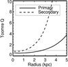 |
Fig. 7 Toomre Q parameter estimated as a function of radius for the initial disk galaxies in a 4:1 merger in ramses. A horizontal line marks the marginally stable value Q = 1. At a gas temperature of 103 K (which is effectively enforced by the Jeans polytrope temperature minimum), the secondary galaxy is substantially more stable than the primary, and it remains stable or near marginal stability at all radii. This leads to a low SFR in the secondary. In the gasoline simulations without a Jeans polytrope, the secondary has higher SFRs. |
3.2.6. Star formation rates
Overall, SFRs during the stochastic phase are similar in the two simulations. In both cases, the total SFRs are dominated by those in the primary galaxies. This dominance is more pronounced in the ramses simulation, as the SFR of the secondary galaxy is quite low (see Fig. 2). Notably, the gas mass within 1 kpc is similar for the two simulations, implying that ramses has a lower star formation efficiency (SFR/Mgas).
We attribute the abnormally low SFR in the secondary ramses galaxy – but not in the primary galaxy – to the pressure support provided by the Jeans polytrope. As described above, the Jeans polytrope acts as a minimum temperature that ensures the Jeans length is always resolved.
As is seen in Fig. 5, the ramses gas density distribution peaks around ~102 cm-3; at this density the temperature floor is around 103 K. We can quantify the stability imposed using an analysis of the Toomre Q parameter (Toomre 1964). In a thin galactic disk, the value of Q quantifies the stability of the disk against gravitational collapse: small values indicate gravitational collapse, large values indicate stability, and Q ≈ 1 indicates marginal instability. We estimate Q as a function of radius using  (1)where vcirc/r is the orbital frequency, vcirc(r) is the circular velocity at radius r, cs is the gas thermal sound speed, G is the gravitational constant, and Σ is the gas surface density in the disk at r3. We calculate cs assuming a gas temperature of 103 K, which is roughly the limit imposed by the Jeans polytrope in ramses.
Figure 7 shows Q as a function of radius for the initial galaxies in the 4:1 merger. The primary galaxy is Toomre-unstable within a radius of ~2.5 kpc. The smaller, secondary galaxy is significantly more stable than the primary, and Q barely reaches below 1 (and only in the central kpc). Thus, the Jeans polytrope stabilizes the smaller gas disk, inhibiting gravitational collapse and star formation.
This stabilization may also help explain why the SFRs near the secondary black hole during the merger phase (after the second pericenter) are lower in ramses than in gasoline. The amount of gas within 1 kpc of the secondary BH is similar in both simulations, but the SFR is lower in ramses (see Fig. 2). Another contributor to the stability at smaller radii could be the presence of the artificially-massive black hole, which would boost the circular velocity and therefore Q. In the primary galaxy, however, we see little evidence for a suppression of the SF efficiency in the central regions of the ramses simulation relative to the gasoline simulation, suggesting that the artificially-massive black hole plays little role. Finally, efficient AGN feedback may help maintain the gas at higher temperatures, suppressing the SF efficiency.
Near the primary BH, at and after the third pericenter, the gas inflow to the central kpc is more significant in gasoline than in ramses. This leads to a larger gas mass and stronger burst of SF in gasoline than in ramses (see Fig. 2). The origin of this difference is unclear. It could result from differences in the dynamics around the black holes, or from the efficient AGN feedback in ramses that evacuates gas from the nuclear regions.
Another possible driver of differences in SFR could be the supernova feedback recipe. In gasoline, gas heated by supernovae is not allowed to cool for a time that depends on local gas conditions. In ramses, the cooling delay is fixed at 20 Myr. Supernova feedback helps regulate star formation, so different SFRs could arise from these different implementations. The primary galaxies have similar SFRs during the stochastic phase of our simulations, so the different supernova feedback seems to have a minor effect.
In summary, the two simulations have similar SFRs overall, but the gasoline simulation shows more SF in the secondary galaxy and during the merger phase than does the ramses simulation. We attribute these differences to stabilization due to the Jeans polytrope in ramses. This temperature floor increases the gas stability against collapse and suppresses star formation.
4. Conclusion
We have compared galaxy merger simulations including black hole growth with ramses, an AMR code, and gasoline, an SPH code, to find which is robust against differences in the codes and their physics implementations. We ran a small suite of new ramses simulations and used gasoline simulations from a suite described in Capelo et al. (2015). In both cases, the simulations had a spatial resolution of ~20 pc and mass resolution of ~5 × 10³M⊙, and included standard subgrid recipes for gas cooling, star formation, supernova feedback, and black hole fueling and feedback.
The simulations show general agreement in their dynamical behavior, and the results are broadly in line with the long-standing picture of galaxy merger simulation evolution (see Di Matteo et al. 2005; Hopkins et al. 2006). Black hole growth is relatively slow while the galaxies are well-separated, including the time between the first and second pericenters. During this phase, black hole growth is driven by stochastic accretion (Hopkins & Hernquist 2006; Gabor & Bournaud 2013; Capelo et al. 2015), just as it is for isolated galaxies. Once the galaxies’ effective radii overlap at the second pericenter, tidal torques trigger gas inflows toward the nucleii. The activity is strongest when the galaxies finally coalesce (beginning at the third pericenter). The inflowing gas, driven to higher densities, initiates peaks in the SFR and the black hole accretion rate.
While the general behavior of the galaxy mergers is similar, there are quantitative differences between simulations run with different codes. We attribute most of these discrepancies to differences in subgrid cooling and feedback models, but effects of the hydrodynamic methods (SPH and AMR) or even gravity solvers (gravity tree and Particle Mesh) may play a role. In ramses simulations, nuclear black holes accrete significantly less than in gasoline, both while the galaxies are well-separated and during coalescence. This arises because of a higher feedback efficiency in ramses that regulates the black hole growth at a lower level. Furthermore, the more efficient black hole feedback ensures that central star formation is lower in ramses during the merger and coalescence. Another difference between codes is the ISM gas structure: in our gasoline simulations gas forms small filaments and collapses into tiny dense knots, whereas in our ramses simulations gas forms thick filaments and large clumps. Gas structure differences are due partly to the inclusion of a Jeans polytrope pressure floor in ramses, though at the smallest scales they are related to numerical methods.
While differences in hydrodynamic method are important in some regimes of galaxy evolution models (e.g., Hayward et al. 2014), we conclude that the most important differences arise in the treatment of baryonic physics (particularly stellar and AGN feedback; Scannapieco et al. 2012).
In future work, simulations like the ones presented here could be improved in several ways. First, the generation of the initial conditions must be treated carefully. One simple way to improve the similarity between the initial conditions would be to generate ramses initial conditions first (because there are more restrictions), then use these in gasoline. Second, differences in gas structures between codes can be minimized by using an identical temperature/pressure floor (i.e., the Jeans polytrope) and tuning the refinement criteria for the adaptive mesh. Choosing to use a Jeans polytrope is a philosophical decision that depends on whether collapsing gas clouds should be treated as subgrid star-forming regions. A reasonable suggestion for the refinement criteria is that the AMR gas cell size should be comparable to particle smoothing lengths throughout the galactic disk, but further work must confirm this. Third, and most importantly, stellar and AGN feedback recipes could be adapted to be more similar, although differences in code structure may make this difficult. For example, AGN feedback could be triggered on the same timescale in both codes (e.g., at every timestep), and the feedback energy could be spread over a fixed gas mass.
Our study underscores that simulation codes that successfully reproduce a range of observables are robust at predicting the same general physical behavior in galaxy mergers; however, one should be careful when comparing quantitatively one particular simulation to one given observable, as these can be model-dependent. The trends, on the other hand, are robust and can be used to obtain physical insights.
Recent improvements to SPH have helped alleviate many of these discrepancies (e.g., Beck et al. 2016 and references therein). Such improvements have recently been implemented in gasoline as described in e.g., Keller et al. (2014).
Our standard boost factor is α = 3 as originally reported in Capelo et al. (2015), but we recently found an error that doubles this boost factor in some segments of some simulations. Since black hole growth is self-regulated by AGN feedback in these simulations, our results are insensitive to the exact boost factor. For example, the difference in black hole accretion between Capelo et al. (2015) and Van Wassenhove et al. (2012), where no boost factor was used (i.e., α = 1), is negligible.
This estimate is accurate for flat rotation curves, for which the epicyclic frequency is  . It is an underestimate of Q in the central kpc of our simulations where the rotation is rising.
Acknowledgments
We thank the referee for suggestions that improved this paper. We acknowledge grant ERC-StG-257720 and GENCI computing resources through project 2192. P.R.C. acknowledges support by the Tomalla Foundation. F.G. acknowledges support from grant AST-1410012 and NASA ATP13-0020. T.Q. acknowledges support from NSF award AST-1311956.
References
- Agertz, O., Moore, B., Stadel, J., et al. 2007, MNRAS, 380, 963 [NASA ADS] [CrossRef] [Google Scholar]
- Barnes, J. E., & Hernquist, L. E. 1991, ApJ, 370, L65 [NASA ADS] [CrossRef] [Google Scholar]
- Barnes, J. E., & Hernquist, L. 1996, ApJ, 471, 115 [NASA ADS] [CrossRef] [Google Scholar]
- Beck, A. M., Murante, G., Arth, A., et al. 2016, MNRAS, 455, 2110 [Google Scholar]
- Bellovary, J. M., Governato, F., Quinn, T. R., et al. 2010, ApJ, 721, L148 [NASA ADS] [CrossRef] [Google Scholar]
- Bellovary, J., Brooks, A., Volonteri, M., et al. 2013, ApJ, 779, 136 [NASA ADS] [CrossRef] [Google Scholar]
- Benson, A. J. 2005, MNRAS, 358, 551 [NASA ADS] [CrossRef] [Google Scholar]
- Berger, M. J., & Colella, P. 1989, J. Comput. Phys., 82, 64 [NASA ADS] [CrossRef] [Google Scholar]
- Bleuler, A., & Teyssier, R. 2014, MNRAS, 445, 4015 [NASA ADS] [CrossRef] [Google Scholar]
- Bondi, H. 1952, MNRAS, 112, 195 [NASA ADS] [CrossRef] [MathSciNet] [Google Scholar]
- Booth, C. M., & Schaye, J. 2009, MNRAS, 398, 53 [NASA ADS] [CrossRef] [Google Scholar]
- Bournaud, F., & Combes, F. 2002, A&A, 392, 83 [NASA ADS] [CrossRef] [EDP Sciences] [Google Scholar]
- Capelo, P. R., Volonteri, M., Dotti, M., et al. 2015, MNRAS, 447, 2123 [NASA ADS] [CrossRef] [Google Scholar]
- Christensen, C., Quinn, T., Governato, F., et al. 2012, MNRAS, 425, 3058 [NASA ADS] [CrossRef] [Google Scholar]
- Crenshaw, D. M., Kraemer, S. B., & George, I. M. 2003, ARA&A, 41, 117 [NASA ADS] [CrossRef] [Google Scholar]
- Croton, D. J., Springel, V., White, S. D. M., et al. 2006, MNRAS, 365, 11 [NASA ADS] [CrossRef] [Google Scholar]
- Debuhr, J., Quataert, E., Ma, C.-P., & Hopkins, P. 2010, MNRAS, 406, L55 [NASA ADS] [Google Scholar]
- Debuhr, J., Quataert, E., & Ma, C.-P. 2011, MNRAS, 412, 1341 [NASA ADS] [Google Scholar]
- Di Matteo, T., Springel, V., & Hernquist, L. 2005, Nature, 433, 604 [NASA ADS] [CrossRef] [PubMed] [Google Scholar]
- Dubois, Y., Devriendt, J., Slyz, A., & Teyssier, R. 2010, MNRAS, 409, 985 [NASA ADS] [CrossRef] [Google Scholar]
- Dubois, Y., Devriendt, J., Slyz, A., & Teyssier, R. 2012, MNRAS, 420, 2662 [NASA ADS] [CrossRef] [Google Scholar]
- Dubois, Y., Volonteri, M., Silk, J., et al. 2015, MNRAS, 452, 1502 [NASA ADS] [CrossRef] [Google Scholar]
- Fabian, A. C., Sanders, J. S., Ettori, S., et al. 2000, MNRAS, 318, L65 [NASA ADS] [CrossRef] [Google Scholar]
- Gabor, J. M., & Bournaud, F. 2013, MNRAS, 434, 606 [NASA ADS] [CrossRef] [Google Scholar]
- Gabor, J. M., & Bournaud, F. 2014, MNRAS, 437, L56 [NASA ADS] [CrossRef] [Google Scholar]
- Gerhard, O. E. 1981, MNRAS, 197, 179 [NASA ADS] [CrossRef] [Google Scholar]
- Gingold, R. A., & Monaghan, J. J. 1977, MNRAS, 181, 375 [Google Scholar]
- Hahn, O., Teyssier, R., & Carollo, C. M. 2010, MNRAS, 405, 274 [NASA ADS] [Google Scholar]
- Hayward, C. C., Torrey, P., Springel, V., Hernquist, L., & Vogelsberger, M. 2014, MNRAS, 442, 1992 [NASA ADS] [CrossRef] [Google Scholar]
- Hernquist, L. 1989, Nature, 340, 687 [NASA ADS] [CrossRef] [Google Scholar]
- Hernquist, L. 1990, ApJ, 356, 359 [NASA ADS] [CrossRef] [Google Scholar]
- Hopkins, P. F. 2014, GIZMO: Multi-method magneto-hydrodynamics+gravity code (Astrophysics Source Code Library) [Google Scholar]
- Hopkins, P. F., & Hernquist, L. 2006, ApJS, 166, 1 [NASA ADS] [CrossRef] [Google Scholar]
- Hopkins, P. F., Hernquist, L., Cox, T. J., et al. 2006, ApJS, 163, 1 [Google Scholar]
- Katz, N. 1992, ApJ, 391, 502 [NASA ADS] [CrossRef] [Google Scholar]
- Keller, B. W., Wadsley, J., Benincasa, S. M., & Couchman, H. M. P. 2014, MNRAS, 442, 3013 [NASA ADS] [CrossRef] [Google Scholar]
- Kereš, D., Vogelsberger, M., Sijacki, D., Springel, V., & Hernquist, L. 2012, MNRAS, 425, 2027 [NASA ADS] [CrossRef] [Google Scholar]
- Khochfar, S., & Burkert, A. 2006, A&A, 445, 403 [NASA ADS] [CrossRef] [EDP Sciences] [Google Scholar]
- Kim, J.-H., Wise, J. H., Alvarez, M. A., & Abel, T. 2011, ApJ, 738, 54 [NASA ADS] [CrossRef] [Google Scholar]
- Kim, J.-H., Abel, T., Agertz, O., et al. 2014, ApJS, 210, 14 [NASA ADS] [CrossRef] [Google Scholar]
- Kormendy, J., & Ho, L. C. 2013, ARA&A, 51, 511 [Google Scholar]
- Krumholz, M. R., McKee, C. F., & Klein, R. I. 2004, ApJ, 611, 399aa25792-15 [NASA ADS] [CrossRef] [Google Scholar]
- Lucy, L. B. 1977, AJ, 82, 1013 [NASA ADS] [CrossRef] [Google Scholar]
- Machacek, M. E., Bryan, G. L., & Abel, T. 2001, ApJ, 548, 509 [NASA ADS] [CrossRef] [Google Scholar]
- Marconi, A., & Hunt, L. K. 2003, ApJ, 589, L21 [NASA ADS] [CrossRef] [Google Scholar]
- McKee, C. F., & Ostriker, J. P. 1977, ApJ, 218, 148 [NASA ADS] [CrossRef] [Google Scholar]
- Mihos, J. C., & Hernquist, L. 1996, ApJ, 464, 641 [NASA ADS] [CrossRef] [Google Scholar]
- Miller, G. E., & Scalo, J. M. 1979, ApJS, 41, 513 [NASA ADS] [CrossRef] [Google Scholar]
- Navarro, J. F., Frenk, C. S., & White, S. D. M. 1996, ApJ, 462, 563 [NASA ADS] [CrossRef] [Google Scholar]
- Negroponte, J., & White, S. D. M. 1983, MNRAS, 205, 1009 [NASA ADS] [CrossRef] [Google Scholar]
- Nelson, D., Vogelsberger, M., Genel, S., et al. 2013, MNRAS, 429, 3353 [NASA ADS] [CrossRef] [Google Scholar]
- Newton, R. D. A., & Kay, S. T. 2013, MNRAS, 434, 3606 [NASA ADS] [CrossRef] [Google Scholar]
- Perret, V., Renaud, F., Epinat, B., et al. 2014, A&A, 562, A1 [NASA ADS] [CrossRef] [EDP Sciences] [Google Scholar]
- Raiteri, C. M., Villata, M., & Navarro, J. F. 1996, A&A, 315, 105 [NASA ADS] [Google Scholar]
- Randall, S. W., Forman, W. R., Giacintucci, S., et al. 2011, ApJ, 726, 86 [NASA ADS] [CrossRef] [Google Scholar]
- Rupke, D. S. N., & Veilleux, S. 2011, ApJ, 729, L27 [NASA ADS] [CrossRef] [Google Scholar]
- Sanders, D. B., Soifer, B. T., Elias, J. H., et al. 1988, ApJ, 325, 74 [NASA ADS] [CrossRef] [Google Scholar]
- Scannapieco, C., Wadepuhl, M., Parry, O. H., et al. 2012, MNRAS, 423, 1726 [Google Scholar]
- Shen, S., Wadsley, J., & Stinson, G. 2010, MNRAS, 407, 1581 [NASA ADS] [CrossRef] [Google Scholar]
- Silk, J., & Rees, M. J. 1998, A&A, 331, L1 [NASA ADS] [Google Scholar]
- Somerville, R. S., Hopkins, P. F., Cox, T. J., Robertson, B. E., & Hernquist, L. 2008, MNRAS, 391, 481 [NASA ADS] [CrossRef] [Google Scholar]
- Springel, V. 2005, MNRAS, 364, 1105 [NASA ADS] [CrossRef] [Google Scholar]
- Springel, V. 2010, MNRAS, 401, 791 [NASA ADS] [CrossRef] [Google Scholar]
- Springel, V., & White, S. D. M. 1999, MNRAS, 307, 162 [NASA ADS] [CrossRef] [Google Scholar]
- Springel, V., Di Matteo, T., & Hernquist, L. 2005, ApJ, 620, L79 [NASA ADS] [CrossRef] [Google Scholar]
- Stadel, J. G. 2001, Ph.D. Thesis, University of Washington, USA [Google Scholar]
- Stinson, G., Seth, A., Katz, N., et al. 2006, MNRAS, 373, 1074 [NASA ADS] [CrossRef] [Google Scholar]
- Teyssier, R. 2002, A&A, 385, 337 [NASA ADS] [CrossRef] [EDP Sciences] [Google Scholar]
- Teyssier, R., Moore, B., Martizzi, D., Dubois, Y., & Mayer, L. 2011, MNRAS, 414, 195 [CrossRef] [Google Scholar]
- Teyssier, R., Pontzen, A., Dubois, Y., & Read, J. I. 2013, MNRAS, 429, 3068 [NASA ADS] [CrossRef] [Google Scholar]
- Toomre, A. 1964, ApJ, 139, 1217 [NASA ADS] [CrossRef] [Google Scholar]
- Toomre, A., & Toomre, J. 1972, ApJ, 178, 623 [NASA ADS] [CrossRef] [Google Scholar]
- Tremmel, M., Governato, F., Volonteri, M., & Quinn, T. R. 2015, MNRAS, 451, 1868 [NASA ADS] [CrossRef] [Google Scholar]
- Truelove, J. K., Klein, R. I., McKee, C. F., et al. 1997, ApJ, 489, L179 [NASA ADS] [CrossRef] [Google Scholar]
- Van Wassenhove, S., Volonteri, M., Mayer, L., et al. 2012, ApJ, 748, L7 [NASA ADS] [CrossRef] [Google Scholar]
- Van Wassenhove, S., Capelo, P. R., Volonteri, M., et al. 2014, MNRAS, 439, 474 [NASA ADS] [CrossRef] [Google Scholar]
- Vogelsberger, M., Sijacki, D., Kereš, D., Springel, V., & Hernquist, L. 2012, MNRAS, 425, 3024 [NASA ADS] [CrossRef] [Google Scholar]
- Voit, G. M., & Donahue, M. 2005, ApJ, 634, 955 [NASA ADS] [CrossRef] [Google Scholar]
- Wadsley, J. W., Stadel, J., & Quinn, T. 2004, New Astron., 9, 137 [NASA ADS] [CrossRef] [Google Scholar]
- Wadsley, J. W., Veeravalli, G., & Couchman, H. M. P. 2008, MNRAS, 387, 427 [NASA ADS] [CrossRef] [Google Scholar]
- Wurster, J., & Thacker, R. J. 2013a, MNRAS, 431, 2513 [NASA ADS] [CrossRef] [Google Scholar]
- Wurster, J., & Thacker, R. J. 2013b, MNRAS, 431, 539 [NASA ADS] [CrossRef] [Google Scholar]
- Wyithe, J. S. B., & Loeb, A. 2003, ApJ, 595, 614 [NASA ADS] [CrossRef] [Google Scholar]
All Figures
|
Fig. 1 Snapshots showing gas surface density for our 4:1 ramses (top) and gasoline (bottom) simulations. Left panels show both galaxies at first apocenter, with arrows roughly indicating the direction of travel of the secondary galaxy. Middle panels show a zoom-in on the primary galaxy at first apocenter, and right panels show both galaxies at the second pericenter. In the right panels, circles mark the positions of the black holes (in each simulation, the more massive black hole is to the left). |
| In the text | |
|
Fig. 2 BH separation in kpc (top), black hole accretion rate (BHAR) in M⊙ yr-1 (second row), gas mass in M⊙ within spheres up to 1 kpc in radius (third row), and SFR in M⊙ yr-1 within the same spheres (bottom row) vs. time for a 4:1 merger with gasoline (left) and ramses (right). For each simulation, we show quantities for the primary galaxy/BH on the left, and the secondary galaxy/BH on the right. We show gas masses and SFRs within radii of 200 pc to 1 kpc, in increments of 200 pc. Quantities are smoothed on 10 Myr timescales. Note that time-axes differ by ~20% (see Sect. 3.2.1). Vertical dotted lines mark local minima in the separation between the two black holes in all panels. The gasoline and ramses simulations show qualitatively similar results: enhanced accretion and star formation rates at the second pericenter, and especially at the third pericenter/coalescence. |
| In the text | |
|
Fig. 3 Face-on images of gas surface density of an isolated disk galaxy simulation using gasoline (left) and ramses (right). The characteristic sizes of gas structures are larger in ramses than in gasoline due partly to the Jeans polytrope pressure floor implemented in ramses and partly to differences in more fundamental aspects of the codes (e.g., hydrodynamic or gravity solvers). |
| In the text | |
|
Fig. 4 Power spectra of gas surface density fluctuations in isolated gasoline and ramses galaxies. The power spectra are normalized by a third-degree power law to highlight the differences between simulations. Shaded error regions indicate the 10–90th percentile range from bootstrap resampling. gasoline shows more power at small scales and less power at large scales, emphasizing that gas structures in our gasoline simulations tend to have smaller sizes than those in ramses. |
| In the text | |
|
Fig. 5 Density-temperature diagrams (top row) and density PDFs (bottom row) for gas in gasoline (left column) and ramses (right column). We show only gas within 500 pc of the primary galactic center in each simulation, and we use a snapshot near the maximum separation (first apocenter, around 500 Myr). In the top panels, we include the temperature distribution along the left axis (arbitrarily normalized and shown on a linear scale). We also schematically show the Jeans polytrope temperature floor for the ramses simulation (straight black line), which keeps the average gas significantly hotter than in gasoline. |
| In the text | |
|
Fig. 6 Gas surface density maps (top) and power spectra (bottom) for ramses simulations of isolated galaxies with different settings: Left: simulation with no Jeans polytrope pressure floor. Right: simulation with a more easily triggered refinement criterion that enables ≈15 pc resolution throughout the galactic disk (and without the Jeans polytrope). Removing the Jeans polytrope ensures that the power on scales ≳200 pc is similar in ramses and gasoline simulations. Enhancing the typical cell size in ramses leads to improved agreement between ramses and gasoline power spectra on scales ≲50 pc at the expense of a discrepancy at moderate scales of ≈50–200 pc (as well as additional computational cost). |
| In the text | |
|
Fig. 7 Toomre Q parameter estimated as a function of radius for the initial disk galaxies in a 4:1 merger in ramses. A horizontal line marks the marginally stable value Q = 1. At a gas temperature of 103 K (which is effectively enforced by the Jeans polytrope temperature minimum), the secondary galaxy is substantially more stable than the primary, and it remains stable or near marginal stability at all radii. This leads to a low SFR in the secondary. In the gasoline simulations without a Jeans polytrope, the secondary has higher SFRs. |
| In the text | |
Current usage metrics show cumulative count of Article Views (full-text article views including HTML views, PDF and ePub downloads, according to the available data) and Abstracts Views on Vision4Press platform.
Data correspond to usage on the plateform after 2015. The current usage metrics is available 48-96 hours after online publication and is updated daily on week days.
Initial download of the metrics may take a while.