| Issue |
A&A
Volume 592, August 2016
|
|
|---|---|---|
| Article Number | A83 | |
| Number of page(s) | 16 | |
| Section | Interstellar and circumstellar matter | |
| DOI | https://doi.org/10.1051/0004-6361/201526991 | |
| Published online | 02 August 2016 | |
Volatile-carbon locking and release in protoplanetary disks
A study of TW Hya and HD 100546⋆,⋆⋆
1 Leiden Observatory, Leiden University, PO Box 9513, 2300 RA Leiden, The Netherlands
e-mail: This email address is being protected from spambots. You need JavaScript enabled to view it.
2 Max Planck Institut für Extraterrestrische Physik, Giessenbachstrasse 1, 85748 Garching, Germany
3 Université de Grenoble Alpes, IPAG, 38000 Grenoble, France
4 CNRS, IPAG, 38000 Grenoble, France
5 INAF-Osservatorio Astrofisico di Arcetri, Largo E. Fermi 5, 50125 Firenze, Italy
6 Max-Planck-Institut für Radioastronomie, Auf dem Hügel 69, 53121 Bonn, Germany
Received: 18 July 2015
Accepted: 17 May 2016
Abstract
Aims. The composition of planetary solids and gases is largely rooted in the processing of volatile elements in protoplanetary disks. To shed light on the key processes, we carry out a comparative analysis of the gas-phase carbon abundance in two systems with a similar age and disk mass, but different central stars: HD 100546 and TW Hya.
Methods. We combine our recent detections of C0 in these disks with observations of other carbon reservoirs (CO, C+, C2H) and gas-mass and warm-gas tracers (HD, O0), as well as spatially resolved ALMA observations and the spectral energy distribution. The disks are modelled with the DALI 2D physical-chemical code. Stellar abundances for HD 100546 are derived from archival spectra.
Results. Upper limits on HD emission from HD 100546 place an upper limit on the total disk mass of ≤0.1 M⊙. The gas-phase carbon abundance in the atmosphere of this warm Herbig disk is, at most, moderately depleted compared to the interstellar medium, with [C]/[H]gas = (0.1−1.5) × 10-4. HD 100546 itself is a λBoötis star, with solar abundances of C and O but a strong depletion of rock-forming elements. In the gas of the T Tauri disk TW Hya, both C and O are strongly underabundant, with [C]/[H]gas = (0.2−5.0) × 10-6 and C / O > 1. We discuss evidence that the gas-phase C and O abundances are high in the warm inner regions of both disks. Our analytical model, including vertical mixing and a grain size distribution, reproduces the observed [C]/[H]gas in the outer disk of TW Hya and allows to make predictions for other systems.
Key words: astrochemistry / protoplanetary disks
Based on observations collected at the European Organisation for Astronomical Research in the Southern Hemisphere under ESO programmes 093.C-0926, 093.F-0015, 077.D-0092, 084.A-9016, and 085.A-9027.
Spectra and models are only available at the CDS via anonymous ftp to cdsarc.u-strasbg.fr (130.79.128.5) or via http://cdsarc.u-strasbg.fr/viz-bin/qcat?J/A+A/592/A83
© ESO, 2016
1. Introduction
Several protoplanetary disks have been found to be depleted of gas-phase CO. This is generally understood to result from the freeze-out of molecules in the midplane and from CO photodissociation in the disk atmosphere (Dutrey et al. 1996, 1997, 2003; van Zadelhoff et al. 2001; Chapillon et al. 2008, 2010). Studies that account for these processes have suggested that the gas is genuinely underabundant in carbon in the disks around HD 100546 and TW Hya (Bruderer et al. 2012; Bergin et al. 2013; Favre et al. 2013; Du et al. 2015). We revisit the gas-phase carbon abundance in these disks, including new detections of far-infrared [C i] lines in the analysis, and present an analytical model for describing the volatile loss.
The solar elemental carbon abundance is [C]/[H] = 2.69 × 10⁻⁴ (Asplund et al. 2009), while the gas-phase abundance in the diffuse interstellar medium is [C]/[H]gas= (1−2) × 10-4 (Cardelli et al. 1996; Parvathi et al. 2012). Several tens of percent of interstellar elemental carbon is locked in refractory solids. Processes affecting the gas and solid carbon budget in disks include the conversion of gas-phase CO into hydrocarbons (e.g. Aikawa et al. 1999; Furuya & Aikawa 2014; Bergin et al. 2014); the freeze out of CO and other carrier molecules (Öberg et al. 2011); the transformation of this icy reservoir into complex organic molecules in cold regions (van Dishoeck 2008; Walsh et al. 2014b); and the vertical transport and oxidation of carbonaceous solids in warm gas (Lee et al. 2010). In our volatile carbon loss model, we include vertical mixing, a vertical and size distribution of dust, and freeze-out.
The composition of a giant planet atmosphere is determined by the gas and dust in the formation or feeding zone of the planet; and by accreted icy planetesimals (Pollack et al. 1996; Chabrier et al. 2014). Formation by gravitational instability involves dust evaporation and produces planets with roughly stellar atmospheric abundances. Core accretion, however, leads to an atmospheric composition determined by the local gas composition, with a potentially large contribution from ablated planetesimals. Determining the gas-solid budget of volatiles in disks is then important for understanding the potential diversity of giant-planet atmospheres, but also for using statistics of planetary compositions as a test of planet population synthesis models (e.g. Pontoppidan et al. 2014; Thiabaud et al. 2015). The gas-solid budget of carbon in a disk may even determine whether or not planets forming in it are habitable from a geophysical viewpoint (Unterborn et al. 2014).
This study is part of the project “Disk carbon and oxygen” (DISCO), aimed at studying the abundance and budget of key elements in planet-forming environments.
2. Observations
Deep integrations of the [C i], CO, C2H and HCO+ transitions, listed in Table 1, towards TW Hya and HD 100546 were obtained with the single-pixel FLASH (Heyminck et al. 2006) and 7-pixel CHAMP+ ([C i] 2–1, CO 6–5) receivers on APEX (Güsten et al. 2006). Observations of TW Hya (ESO proposal E-093.C-0926A, PI M. Kama) totalled 9.1 h in September 2014, with a typical water vapour column of PWV ≈ 1.4 mm. HD 100546 (Max Planck proposal M0015_93, PI E. F. van Dishoeck) was observed from April to July 2014, with PWV ≈ 0.75 mm. The backends were AFFTS (with a highest channel resolution of 0.18 MHz or 0.11 km s-1 at 492 GHz) and XFFTS (FLASH, 0.04 MHz or 0.02 km s-1). Initial processing was done using the APECS software (Muders et al. 2006). Inspection, baseline subtraction and averaging were done with GILDAS/CLASS1. Telescope parameters were obtained from Güsten et al. (2006). The kelvin to jansky conversion and main-beam efficiency at 650 GHz (CHAMP+-I) are 53 Jy K-1 and 0.56, respectively. At 812 GHz (CHAMP+-II), they are 70 Jy K-1 and 0.43. At 491 GHz (FLASH460), the conversion factor is 41 Jy K-1 and ηmb = 0.73. The [C i] detections shown in Fig. 1 and the CO 6–5 detections were presented, but not analyzed in detail, as part of a large survey in Kama et al. (2016).
New observations of TW Hya and HD 100546 with APEX.
Supplementary archival optical spectra were used to perform a chemical abundance analysis of the photosphere of HD 100546. Spectra from FEROS (Kaufer et al. 1999) were extracted from the ESO Science Archive. FEROS is an echelle spectrograph mounted on the MPG/ESO 2.2 m Telescope in La Silla. The instrument has a resolving power of R ~ 48 000 and covers a wavelength range of 360–920 nm in 39 spectral orders. The spectra were obtained in projects E-077.D-0092A, E-084.A-9016A, and E-085.A-9027B, in June 2006, March 2010, and May-June 2010, respectively. The reduced spectra extracted from the ESO Science Archive were continuum normalized by fitting a low order polynomial through carefully selected points. This was done for the individual spectral orders independently, then the normalized spectra were merged. The ten available observations were co-added to boost our final signal-to-noise ratio, since no variability was found in the spectra outside of emission lines. The derivation of photospheric abundances from these data is described in Appendix A.
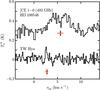 |
Fig. 1 [CI] 1−0 line in HD 100546 (offset by + 0.3 K) and TW Hya. Horizontal bars mark the systemic velocities, 5.70 and 2.86 km s-1. Red crosses show the best-fit Gaussian vlsr with 3σ error bars. The data are binned to 0.14 km s-1 per channel. |
3. The sources
Both of the targeted disks are relatively old (τ ~ 10 Myr) and have a similar dust mass (Mdust ~ 10-4 M⊙). The stellar effective temperatures and luminosities are, however, very different – 4110 K and 0.28 L⊙ for TW Hya and 10 390 K and 36 L⊙ for HD 100546 – providing an opportunity to compare two similar, isolated disks with a very different average dust temperature. The properties of the two sources are summarized in Table 2.
HD 100546 is a (2.4 ± 0.1) M⊙ disk-hosting star of spectral type B9V, with an estimated age of ≳ 10 Myr (van den Ancker et al. 1997). The distance, measured with Hipparcos, is 97 ± 4 pc (van Leeuwen 2007). For its stellar properties and spectrum, including X-ray and UV, we adopt the values of Bruderer et al. (2012, and references therein). We note that the observed total luminosity of HD 100546, 36 L⊙, is larger than the (25 ± 7) L⊙ obtained from the photospheric abundance analysis in Appendix A, where the far-UV data were not included.
The observable dust mass is ≈10-4 M⊙ (Henning et al. 1998; Wilner et al. 2003; Panić & Hogerheijde 2009; Mulders et al. 2011, 2013). Micron-sized grains are observed out to 1000 au (Pantin et al. 2000; Augereau et al. 2001; Grady et al. 2001; Ardila et al. 2007), while millimetre-sized grains are abundant within 230 au and the molecular gas, traced by CO isotopologs, extends to 390 au (Panić & Hogerheijde 2009; Panić et al. 2010; Walsh et al. 2014a). The dust disk inclination is 44° ± 3°. Large dust grains are depleted inside of 13 au, and again from 35 to 150 au (e.g. Bouwman et al. 2003; Walsh et al. 2014a), with a small inner disk from 0.26 to 0.7 au containing 3 × 10⁻¹⁰ M⊙ of dust (Benisty et al. 2010; Panić et al. 2014). The inner hole and outer gap are consistent with radial zones cleared partly of material by two substellar companions (Walsh et al. 2014a).
TW Hya is considered to be a K7 spectral type pre-main sequence star with a mass of 0.8 M⊙, radius 1.04R⊙, Teff= 4110 K and a luminosity 0.28L⊙; although there is some debate regarding these parameters (e.g. Vacca & Sandell 2011; Andrews et al. 2012; Debes et al. 2013). The distance is (55 ± 9) pc (van Leeuwen 2007) and the age ~8−10 Myr (e.g. Hoff et al. 1998; Webb et al. 1999; de la Reza et al. 2006; Debes et al. 2013).
The disk-gas mass was recently estimated from HD emission to be ≳ 0.05 M⊙ (Gorti et al. 2011; Bergin et al. 2013). An inner disk extends from 0.06 to 0.5 au, followed by a radial gap in continuum opacity out to 4 au (Calvet et al. 2002; Eisner et al. 2006; Hughes et al. 2007; Akeson et al. 2011; Andrews et al. 2012). The disk extends to ≳280 au in scattered light, while the large grains are seen only out to 60 au in 870 μm emission and the CO gas is within 215 au (Andrews et al. 2012). The inclination is 7° ± 1° (Qi et al. 2004; Hughes et al. 2011; Andrews et al. 2012; Rosenfeld et al. 2012). Scattered light imaging with HST at 0.5 to 2.2 μm reveals a 30% intensity gap in the radial brightness distribution at ~80 au, consistent with a 6 to 28M⊕ companion (Debes et al. 2013). Another gap has recently been suggested at ~20 au (Akiyama et al. 2015).
The accretion luminosity is estimated to be 0.03 L⊙, but estimates of the accretion rate vary from 4 × 10⁻¹⁰ to 4.8 × 10⁻⁹ M⊙ yr-1 (Muzerolle et al. 2000; Batalha et al. 2002; Kastner et al. 2002; Debes et al. 2013). The X-ray luminosity is 1.4 × 1030 erg s-1, originating in a two-temperature plasma with a main peak at TX = 3.2 × 10⁶ K and a secondary at ≳3.2 × 10⁷ K (Kastner et al. 2002; Brickhouse et al. 2010).
4. Overview of the spectra
The CO 6–5, [C i] 1–0 and HCO+4–3 transitions are detected towards both TW Hya and HD 100546, while C2H is detected only towards TW Hya (Table 1). The [C i] 1–0 spectra are shown in Fig. 1. The emission towards HD 100546 is double-peaked, with symmetric peaks for [C i] and a slightly stronger blue- than redshifted peak for CO 6–5, which is consistent with previous CO observations (e.g. Panić et al. 2010) and with the inclination. Based on an extended scattered light halo and single-peaked [C ii] emission, a compact, tenuous envelope is thought to surround the HD 100546 disk (Grady et al. 2001; Bruderer et al. 2012; Fedele et al. 2013b). The CO 6–5 and [C i] 1–0 lines are double-peaked, indicating they are not contaminated by the envelope. As described in Appendix B, we used a set of offset pointings to further verify that the CO 6–5 and [C i] 1–0 transitions do not have a substantial envelope emission contribution. The line profiles towards TW Hya are single-peaked and narrow, consistent with its low inclination. The [C i] line peaks at 2.7 ± 0.3 km s-1 (3σ), consistent with the canonical systemic velocity of 2.86 km s-1. The C2H line fluxes for TW Hya are consistent with those from Kastner et al. (2014, 2015).
The detections of [C i] 1–0 represent the first unambiguous detections of atomic carbon in protoplanetary disks in the far-infrared. The line was detected previously towards DM Tau by Tsukagoshi et al. (2015) and Kama et al. (2016), however it is single-peaked and narrower than the double-peaked CO profiles seen from that source, which suggests contamination by a compact residual envelope and requires further follow-up.
Our new data, listed in Table 1, were supplemented with continuum and spectral line data from the literature, listed in Appendix C.
5. Analysis
To derive the gas-phase abundance of elemental carbon ([C]/[H]gas), we have run source-specific model grids using the 2D physical-chemical code, DALI (Bruderer et al. 2009, 2012; Bruderer 2013). The code uses Monte Carlo radiative transfer to determine the dust temperature. The gas-grain chemistry in each grid cell is then solved time-dependently. For the grain surface chemistry, only hydrogenation is considered. The steady-state heating-cooling balance of the gas is determined at each time-step. We let the chemistry evolve to 10 Myr to match the ages of the two disks.
The disk structure is parameterized as shown in Fig. 2. We denote the gas-to-dust mass ratio as Δgas / dust. The dust consists of a small (0.005–1 μm) and large (0.005–1 mm) grain population. The surface density profile is a power law with an exponential taper: ![Mathematical equation: \begin{equation} \Sigma_{\rm gas} = \Sigma_{\rm c}\times \left( \frac{r}{R_{\rm c}} \right)^{-\gamma} \times \exp{\left[- \left(\frac{r}{R_{\rm c}}\right)^{2-\gamma} \right]}\cdot \end{equation}](/articles/aa/full_html/2016/08/aa26991-15/aa26991-15-eq137.png) (1)Σgas and Σdust extend from the dust sublimation radius Rsub to Rout and can be independently varied inside the radius Rcav with the multiplication factors δgas and δdust. Dust is depleted entirely from Rgap to Rcav. The scaleheight angle, h, at distance r is given by h(r) = hc (r/Rc)ψ. The scaleheight is then H = h·r, and the vertical density distribution of the small grains is given by
(1)Σgas and Σdust extend from the dust sublimation radius Rsub to Rout and can be independently varied inside the radius Rcav with the multiplication factors δgas and δdust. Dust is depleted entirely from Rgap to Rcav. The scaleheight angle, h, at distance r is given by h(r) = hc (r/Rc)ψ. The scaleheight is then H = h·r, and the vertical density distribution of the small grains is given by ![Mathematical equation: \begin{equation} \label{eq:rhosmall} \rho_{\rm dust,small} = \frac{(1-f)\,\Sigma_{dust}}{\sqrt{2\,\pi}\,r\,h} \times \exp{ \left[-\frac{1}{2} \left( \frac{\pi/2 - \theta}{h} \right)^{2} \right] }, \end{equation}](/articles/aa/full_html/2016/08/aa26991-15/aa26991-15-eq150.png) (2)where f is the mass fraction of large grains, and θ is the opening angle from the midplane as viewed from the central star. The settling of large grains is prescribed as a fraction χ ∈ (0,1] of the scaleheight of the small grains, so the mass density of large grains is similar to Eq. (2), with f replacing (1−f) and χh replacing h. The vertical distribution of gas is ρgas = Δgas / dust × ρdust,small × [1 + f/ (1−f)]. The term f/ (1−f) preserves the global Δgas / dust outside Rcav.
(2)where f is the mass fraction of large grains, and θ is the opening angle from the midplane as viewed from the central star. The settling of large grains is prescribed as a fraction χ ∈ (0,1] of the scaleheight of the small grains, so the mass density of large grains is similar to Eq. (2), with f replacing (1−f) and χh replacing h. The vertical distribution of gas is ρgas = Δgas / dust × ρdust,small × [1 + f/ (1−f)]. The term f/ (1−f) preserves the global Δgas / dust outside Rcav.
First, we fit the spectral energy distribution (SED), also varying δgas and δdust in the inner cavities of both disks. Combined, the SED, the resolved CO 3–2 emission profile, and the CO ladder and [O i] lines constrain Σdust, hc, ψ, γ, f, χ, the properties of any large inner hole, and to some extent Δgas / dust. Fluxes or upper limits of HD lines constrain the mass of warm gas (see also Bergin et al. 2013). The spectral line profiles of CO and [C i] further constrain the disk temperature and density structure, as well as the stellar mass and the disk inclination. Finally, modelling the CO ladder, the [C i], [C ii] and [O i] lines constrains [C]/[H]gas as well as the C/O ratio, although in HD 100546 the [C ii] and [O i] lines are contaminated by envelope emission. We vary [O]/[H]gas either in lockstep with [C]/[H]gas (fixed C/O ratio), or keep it fixed at 2.88 × 10⁻⁴ for variations of [C]/[H]gas. The use of DALI to derive [C]/[H]gas is described in more detail in Kama et al. (2016). The two main sources of uncertainty are the radial extent of the gas disk and the gas to dust ratio.
Both of our target disks show evidence for radial gaps in the millimetre opacity. We have not included these in our current modelling, as the thermal structure of both disks is more strongly related to the small grains, traced by scattered light. Shallow radial dips and wave patterns are seen in scattered light (e.g. Ardila et al. 2007; Debes et al. 2013), but it is not clear that these represent large variations of UV heating and thus do not yet warrant inclusion in our modelling.
Next, we describe the results of modelling each system. The range of well-fitting values for each parameter is listed in Table 2, and the disk structures and abundance maps are shown in Appendix D. The stellar spectra are from Bruderer et al. (2012), France et al. (2014) and Cleeves et al. (2015), and their UV profile is shown in Fig. 3. Blackbody spectra of pre main-sequence model stars from Tognelli et al. (2011) for an age of 10 Myr are provided for comparison. To illustrate the importance of accretion power, we added UV excess to the 4000 K star corresponding to 10-9 and 10-8 M⊙ yr-1 of mass flux emitting its complete potential energy at the stellar surface at a temperature of 10 000 K. The stellar luminosities are summarized in Table 3. The range of well-fitting models was chosen by eye through consecutive parameter value refinements totalling about 100 models per source.
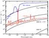 |
Fig. 3 The ultraviolet range of spectra used in this study for TW Hya (red curve, France et al. 2014; Cleeves et al. 2015) and HD 100546 (blue curve, Bruderer et al. 2012), compared with blackbody photospheres for pre main sequence model stars with an age of 10 Myr (black curves, Tognelli et al. 2011). The two curves labelled 4000 K+UV show a 4000 K stellar photosphere with a 10 000 K blackbody added for the accretion rates Ṁ= 10-9 and 10-8 M⊙ yr-1. See also Table 3. |
Total and ultraviolet stellar luminosities for TW Hya and HD 100546 and a set of model stars with blackbody spectra.
5.1. HD 100546: carbon and oxygen are close to interstellar
The results for HD 100546 are shown in Fig. 4. Maps of the abundance and line emission of key species for the best-fit model with [C]/[H]gas= 10-4 and a Δgas / dust= 10 are shown in Fig. D.1. We show the SED (top left panel), the [C i] 1–0 and CO 3–2 and 6–5 line profiles (top middle), the radial cut of CO 3–2 intensity from ALMA (top right) and the compilation of spectral line fluxes (bottom panel). The disk is vertically extended and warm.
We obtain 10 ≤ Δgas / dust ≤ 300 for the outer disk. The upper limit relies on the HD 1–0 (112 μm) and 2–1 (56 μm) upper limits calculated from the PACS spectrum of Fedele et al. (2013a). This is ≲ 0.1 M⊙ or Δgas / dust ≲ 300, adopting our best fit dust mass of 8.1 × 10⁻⁴ M⊙. The corresponding surface density law is Σgas ≲ 150 (r/ 50 au)-1g cm-2. Having Δgas / dust< 10 requires [C]/[H]gas≳ 2 × 10⁻⁴ to match the CO lines which, however, leads to the atomic carbon lines being overpredicted.
We find [C]/[H]gas = (0.1−1.5) × 10-4 and a C/O ratio that is solar to within a factor of a few. This uncertainty is mostly due to the limited constraints on the gas to dust ratio. An interstellar-like carbon abundance ([C]/[H]gas~ 10-4 in the diffuse ISM) provides a good fit if Δgas / dust~ 10. For this model, additionally, the oxygen abundance must be ≳10-4, otherwise the [C i] line fluxes are substantially overpredicted as less carbon is bound into CO. Therefore, for the low gas to dust ratio and nominal [C]/[H]gas solution, [O]/[H]gas must also be roughly interstellar. For Δgas / dust = 100, the best-fit value for [C]/[H]gas is ~2 × 10⁻⁵, assuming a solar C/O ratio. For this Δgas / dust, a carbon abundance of 10-4 overproduces the CO ladder by a factor of ten and the [C i] detection by a factor of two. Decreasing the oxygen abundance such that the C/O ratio is above unity improves the fit on the CO ladder, but leads to an even more substantial overprediction of the [C i] 1–0 transition.
Using the dust disk model of Mulders et al. (2011) and a wide range of constraints on the disk and stellar properties, Bruderer et al. (2012) modelled [C ii], [O i] and CO (Ju ≥ 14) fluxes and [C i] upper limits. They found gas-to-dust ratios from 20 to 100 and corresponding [C]/[H]gas values of 1.2 × 10⁻⁴ (interstellar) to 1.2 × 10⁻⁵ (depleted from the gas by a factor of ten). Our results from above are consistent with these values.
Our analysis of the stellar photospheric abundance (Appendix A) is consistent with the star accreting carbon-rich gas, as would be expected in a system where volatile carbon is not depleted from the gas into planetesimals. We return to this in Sect. 6.3.
The [O i] 63 μm and 145 μm lines are always underproduced by factors of two to four, and the spectrally resolved [C ii] emission by a factor of approximately five. The latter line is single-peaked and very likely contains substantial emission from a residual circum-disk envelope (e.g. Fedele et al. 2013b,a; Dent et al. 2013). As a consistency check, we calculate the envelope emission assuming nH2= 104 cm-3, a spherical radius of 103au and an abundance 10-4 of both O0 and C+. Assuming Tkin ~ 50 to 150 K, the missing flux is recovered with such an envelope model.
We adopt the Δgas / dust = 10 and [C]/[H]gas = 10-4 model for HD 100546 in the rest of the paper, unless explicitly noted.
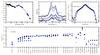 |
Fig. 4 Observations and modelling of HD 100546. The panels show, from top left to bottom, the spectral energy distribution; spectrally resolved line profiles; spatially resolved integrated CO 3–2 emission; and the full set of line fluxes used in the analysis. CO isotopolog lines for a given rotational transition are plotted at the same x-axis location. Two well-fitting models, with a gas to dust ratio Δgas / dust = 10 and [C]/[H]gas = 10-4 (solid blue) and Δgas / dust = 100 and [C]/[H]gas = 10-5 (dashed/open blue) are plotted on the observations (black) to illustrate the range of allowed parameters. The data and model values for C2H have been multiplied by a factor of 103 for display purposes. |
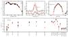 |
Fig. 5 Observations and modelling of TW Hya. The panels show, from top left to bottom, the spectral energy distribution; spectrally resolved line profiles; spatially resolved integrated CO 3–2 emission; and the full set of line fluxes used in the analysis. CO isotopolog lines for a given rotational transition are plotted at the same x-axis location. Two well-fitting models, both with a gas to dust ratio Δgas / dust = 100 and [C]/[H]gas = 10-6 but with C/O = 0.47 (solid red) and 1.5 (dashed/open red) are plotted on the observations (black) to illustrate the range of allowed parameters. For C/O = 0.47, the [O i] 63 μm line model flux lies just above 10-16W m-2 and the C2H fluxes are a factor ≈ 103 below the observations. |
5.2. TW Hya: carbon and oxygen are underabundant
The results for TW Hya are shown in Fig. 5. Maps of the abundance and line emission of key species for a typical well-fitting model, with [C]/[H]gas= 10-6, are shown in Fig. D.2. We show the SED (top left panel), the [C i] 1–0 and CO 3–2 and 6–5 line profiles (top middle), the radial cut of CO 3–2 intensity from ALMA (top right) and the compilation of spectral line fluxes (bottom panel). Constrained by the spatially resolved CO 3–2 data (Rosenfeld et al. 2012), our best-fit models have a radially steeper temperature profile and smaller radius than the models of Cleeves et al. (2015).
TW Hya was the first disk where the gas mass was constrained using the HD 112 μm transition (Bergin et al. 2013). Our best-fit disk mass, Mdisk = 2.3 × 10⁻² M⊙, is within a factor of two of the original range (≥5 × 10⁻² M⊙). An additional feature of our model is that it reproduces the HD 56 μm line, which will be presented in a forthcoming paper (Fedele, in prep.).
The carbon and oxygen abundances are constrained to be low by the combination of [C i], [O i] and low-J CO lines and the HD 112 μm line. The C18O 2–1 flux is another strong constraint on [C]/[H]gas. However, our model does not yet include the isotopolog-selective photodissocation of CO, which may lead to an underestimation of [C]/[H]gas or of the total gas mass (Miotello et al. 2014). Since HD constrains the gas mass, in our case the uncertainty of a factor of a few falls on [C]/[H]gas, but is somewhat mitigated by the complementary constraints from [C i] and [C ii]. We will return to this in a companion paper (Miotello et al. in prep.). Overall, we find that both carbon and oxygen must be substantially underabundant in the gas, with a [C]/[H]gas ratio of (0.2−5.0) × 10-6. The [O]/[H]gas ratio is constrained to be ~10-6. A higher value strongly overpredicts the [O i] 63 μm flux, while a much smaller value leads to an excess of C0 and C2H, as carbon normally bound into CO becomes available.
The Herschel/PACS upper limits on the high-J CO lines (Kamp et al. 2013) also constrain [C]/[H]gas< 10-4. The CO 23–22 line is formally detected, but a recent re-analysis (D. Fedele, priv. comm.) suggests it is blended with an H2O line and we thus treat it as an upper limit.
Based on C18O emission and the HD gas mass, an elemental gas-phase carbon and oxygen deficiency of a factor of 10–100 was already inferred for this disk (Hogerheijde et al. 2011; Bergin et al. 2013; Favre et al. 2013; Du et al. 2015). Our models confirm these results.
5.3. Modelling of C2H and constraining the C/O ratio
C2H is another tracer of the carbon chemistry in the disk surface layers. The hydrocarbon chemistry in our network extends only up to C2H and C2H2. In addition to data from UMIST06, we include the reactions C2H + H2 → C2H2 + H, with an activation barrier of Ea = 624 K (UMIST12), and C2 + H2 → C2H + H, with Ea = 1469 K (Cernicharo 2004), but their effect on the results is not substantial. We note the latter reaction has been studied at high pressure, and the rate may not apply at disk conditions. The ring-like morphology of C2H emission around TW Hya led Kastner et al. (2015) to invoke the photodestruction of hydrocarbons and small carbonaceous grains as a source. We have not included this process in our network.
In the fitting described above, we keep the C/O ratio at the solar value. This underproduces the C2H fluxes in TW Hya by a factor of 100, while the upper limits for C2H in HD 100546 are a factor 1000 above the models. The C2H abundance may be enhanced or decreased depending on the carbon-to-oxygen ratio of the gas. If C/O ≳ 1, hydrocarbons start to become much more abundant. To test this, we ran models with a decreased [O]/[H]gas, making C/O = 1.5. For TW Hya, this makes the modelled C2H fluxes consistent with the observations and somewhat improves the match for [O i]. We plot the results in Fig. 5. For HD 100546, however, the models now lie a factor of fifty above the observational upper limits. Qualitatively, we can conclude that the models suggest a stronger depletion of oxygen than carbon in the outer disk gas of TW Hya, while for HD 100546 there is no evidence for such a differential depletion. Full modelling of C2H is outside the scope of this paper.
6. Locking and release of volatiles in disks
We have confirmed earlier findings by Bruderer et al. (2012), Favre et al. (2013), and Du et al. (2015) that the gas-phase volatile carbon and oxygen are underabundant by two orders of magnitude in the TW Hya disk, while they are roughly interstellar or moderately underabundant in HD 100546. In Fig. 6, we compare the derived [C]/[H]gas ranges for these disks with the photospheric abundance of carbon in HD 100546 and in a large sample of other Herbig Ae/Be stars (Acke & Waelkens 2004; Folsom et al. 2012), as well as with the interstellar and solar carbon abundances (Asplund et al. 2009; Cardelli et al. 1996; Parvathi et al. 2012). The photospheric value for HD 100546 is consistent with the rest of the Herbig star sample, while the [C]/[H]gas ratio in the disk gas is consistent with interstellar or slightly sub-interstellar values. We find no solution for the TW Hya disk in which the [C]/[H]gas value is close to interstellar.
The identified pattern – a strong underabundance in a cold disk and at most moderate underabundance in a warm disk – is consistent with a scenario where vertical mixing transports gas from the disk surface into the cold midplane, where CO, H2O, hydrocarbons and perhaps other C and O carriers can freeze out onto dust grains. We show the main aspects of the depletion for TW Hya in Fig. 7, where the relevant parameters are shown as a function of height at r = 100 au. Our measurement of [C]/[H]gas relies strongly on [C i] and CO emission, and probes mainly the outer disk atmosphere. To remove carbon atoms from this region, they must be transported to the cold midplane, where some of them must then remain. We propose that the systematic loss of carbon is as a result of freeze-out onto grains which are sufficiently decoupled to have scaleheights smaller than the CO freeze-out height (CO snow-surface, the vertical location where Tdust= 17 K). Below, we model this sequestration process and constrain the nature of the main carrier species that freeze out. Finally, we discuss evidence for the evaporation of volatile ices in the warm inner disk of TW Hya.
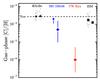 |
Fig. 6 Gas-phase carbon abundance, compared with that of the Sun (dashed line, Asplund et al. 2009). From left to right: photospheric values for Herbig Ae/Be stars (Acke & Waelkens 2004; Folsom et al. 2012, stars); the stellar and disk values for HD 100546 (star and diamond, this work); the disk of TW Hya (diamond, this work); and lines of sight through the diffuse interstellar medium (Cardelli et al. 1996; Parvathi et al. 2012). For the Herbig Ae/Be and ISM samples, the median (black symbols) and the full dataset (small grey circles) are shown. |
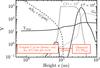 |
Fig. 7 Vertical structure of the TW Hya model at r = 100 au. Y denotes either the dust temperature (Tdust [K]), UV-field (G0), gas-phase CO and C0 abundance, or the grain size (a [μm]) of particles with a scaleheight hd equal to a given height z (see Eq. (5)). Vertical mixing can transport carbon atoms from the C0 layer to the freeze-out zone. |
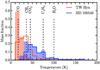 |
Fig. 8 Histograms of the fractional gas (solid lines) and dust mass (shaded) in 10 K temperature bins for the full disk of TW Hya (red) and HD 100546 (blue). Freeze-out temperatures of the main species for C and O loss from the gas to ices are marked with vertical dashed lines. |
6.1. In what form does volatile carbon freeze out?
What species are the main gas-phase carriers that contribute to the loss of carbon to midplane ices? One possible explanation is that the CO+He+ → C+ reaction can liberate carbon from CO in the disk atmosphere. Through reactions with H2, electrons, and C0, hydrocarbon species are then produced (Aikawa et al. 1999). These may become important reservoirs of gas-phase carbon (Bergin et al. 2014; Furuya & Aikawa 2014). Alternatively, the sequestration into ices may start with the mixing and freeze-out of CO itself. In Fig. 8, we show histograms of the dust and gas mass fraction in temperature bins of 10 K for our best models of both disks. We can now test which species dominate the loss of volatile carbon from the gas phase in the outer disk. The main agent of underabundance should condense in the colder disk (TW Hya), but not in the warmer one (HD 100546). Note that the freeze-out is controlled by the dust temperature.
Using C2H2 as a lower limit for large hydrocarbons, for which the sublimation temperature generally increases with size (e.g. Chickos et al. 1986), we see that this class is ruled out as a major gas-phase C carrier. C2H2 is easily able to freeze out in both disks. Some fraction of carbon may be lost as CH4 and CO2, but they are probably not the dominant gas-phase carriers, as both can freeze out in the outer disk of HD 100546. Most gas-phase carbon atoms in the HD 100546 disk have, therefore, not passed through a complex hydrocarbon molecule during the 10 Myr life of the system. This is consistent with chemical models, where CH4 production usually requires long timescales and CO2 is produced by thermal or photo-processing of CO-, H2O-, and OH-rich ices (e.g. Willacy et al. 1998; Furuya et al. 2013; Walsh et al. 2014b). Observable gas-phase complex organic molecules in the protostellar source Orion KL only contain ≲15% of the organic carbon locked in solar system meteorites and comets, suggesting that large amounts of complex organics are produced from simple carbon-bearing species during the protoplanetary disk stage (Bergin et al. 2014). All evidence thus indicates that carbon is lost from the outer disk gas predominantly as CO, which is able to freeze out in a large mass fraction of the TW Hya disk, but not in HD 100546. Further grain surface processing of carbon in ices starts from this parent species. The formation of large amounts of complex organics from this is only possible in disks cold enough for CO freeze-out.
Figure 8 raises the question of the gas-phase oxygen abundance in the HD 100546 disk, as both disks easily allow for near-complete H2O freeze-out. This should facilitate the sequestering of oxygen into midplane ices. In TW Hya, most water ice was indeed inferred to be trapped in the midplane, based on the low H2O line fluxes observed with Herschel (Hogerheijde et al. 2011). Upper limits on H2O emission towards HD 100546 (Sturm et al. 2010; Thi et al. 2011; Meeus et al. 2012; Fedele et al. 2013a) still allow an interstellar gas-phase oxygen abundance, [O]/[H]gas= 2.88 × 10⁻⁴, given our best-fitting disk model. A recent H2O detection in HD 100546 will provide stronger constraints on [O]/[H]gas (Hogerheijde et al., in prep., see also van Dishoeck et al. 2014).
6.2. An analytical model of volatile locking
Two orders of magnitude of gas-phase carbon have been lost from the gas disk of TW Hya, and the processes responsible are likely general and operating on large scales. We present an analytical model for the loss of volatile carbon in a disk, relating a progressing depletion to vertical mixing, freeze-out (ostensibly of CO), and the dust size distribution.
Let r be a radial location in the disk. We assume that gas and the small grains that couple to it at r are constantly vertically mixed, such that they cycle between the disk atmosphere and the midplane. We can remain agnostic as regards the vertical mixing mechanism, as long as the round-trip mixing time tmix can be estimated. In each mixing cycle, let a fraction ΔX of volatiles become permanently locked in the midplane. Assuming the mixing or diffusion cycle lasts tmixyears and the process repeats for a duration of ttotyears, we have N = ttot/tmix cycles. The initial abundance X0 of an element in the disk surface gas will then be depleted to a lower abundance 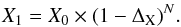 (3)The age of TW Hya is ttot = 10 Myr. We adopt a turbulent mixing time tmix = h2/να, where να = αcsh is the parameterized viscosity of Shakura & Sunyaev (1973), and further set α = 0.01. Taking the disk atmosphere height h, defined here as the region with peak C0 abundance, at r = 100 au to be 30 au (Fig. D.2) and the sound speed cs = 300 m s-1, we find tmix = 5 × 10⁴yr. The left-hand panel of Fig. 9 shows ΔX and N which satisfy X0/X1 = 100 (Eq. (3)). An underabundance of a factor of X0/X1 = 100 over 10 Myr corresponds to Nmix = 200 and a fractional loss per mixing cycle of ΔX = 2 × 10⁻². In one cycle, 98% of the atoms either do not freeze out, or freeze onto grains that are well coupled to the gas and return to the warm disk atmosphere where they desorb.
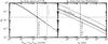 |
Fig. 9 Model of volatile loss from the disk atmosphere. Left-hand panel: a fraction ΔX of volatile atoms are lost in the midplane during each of Nmix mixing cycles. Equation (3) is shown for a depletion X0/X1 = 100 (solid curve). A theoretical turbulent mixing timescale gives Nmix = 200 (black dashed line) and ΔX = 2 × 10⁻² (dotted line), consistent with an upper limit of vturb ≤ 40 m s-1 on the speed of turbulent mixing in TW Hya, which gives Nmix ≤ 1300 (gray dashed line, Hughes et al. 2011). Right-hand panel: ΔX from Eq. (4), taking amax = 10 cm and amin = 0.001, 0.005, or 0.05 μm (solid lines). The smallest grain size settled below the CO freeze-out height at r = 100 au in our TW Hya model is also shown (dashed line, Eq. (5)). |
We interpret the carbon loss term, ΔX, as freeze-out onto large grains which are settled below the height where volatile carbon freezes out. The likeliest candidate carrier is CO, which freezes out in TW Hya at 17 K (Qi et al. 2013). Volatiles that freeze onto grains which have a scaleheight equal to or smaller than the CO snow-surface, where hd = zfreeze−out (this happens at Tdust = 17 K; see also Eq. (5) and Fig. 7), stay locked as ices in the midplane, while ices formed on smaller grains eventually get mixed back to the warm surface layers where they desorb. The loss term ΔX is equal to the fraction of dust surface area contributed by grains which are settled below the CO snowline. We adopt a standard dust size distribution of the form dn/ da = C × a-3.5 between amin = 0.005 μm and amax = 10 cm, where C is a constant, and denote the size of the smallest grains which satisfy hd(ah) = zfreeze−out as amin ≤ ah ≤ amax. We note that the maximum grain size here exceeds that used in the opacities in Sect. 5.2. Assuming that the total surface area of dust above the CO snowline is negligible compared to that below it, we arrive at 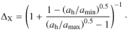 (4)This expression for ΔX is plotted in the right-hand panel of Fig. 9 as ΔX(ah). Based on Youdin & Lithwick (2007), we also plot the grain size at which the dust scaleheight equals the CO snow-surface of z ≈ 8 au. This is ah = 20 μm, obtained from
 ![Mathematical equation: \begin{equation} \label{eq:hdz} \frac{h_{\rm d}(a_{\rm h})}{h_{\rm gas}} = \left[\left( 1 + \frac{ \Omega\, t_{\rm fric}(a_{\rm h}) }{ \alpha }\right)\, \left( \frac{ 1 + 2\,\Omega\, t_{\rm fric}(a_{\rm h}) }{ 1 + \Omega\, t_{\rm fric}(a_{\rm h}) } \right) \right]^{-1/2}, \end{equation}](/articles/aa/full_html/2016/08/aa26991-15/aa26991-15-eq359.png) (5)where hgas = 11 au is the gas scaleheight at 100 au in our TW Hya model, and Ω is the Keplerian frequency at the radial location, Ω(r = 100 au) ≈ (10-10/π) s-1 in our case. The stopping time in the Epstein regime is
(5)where hgas = 11 au is the gas scaleheight at 100 au in our TW Hya model, and Ω is the Keplerian frequency at the radial location, Ω(r = 100 au) ≈ (10-10/π) s-1 in our case. The stopping time in the Epstein regime is 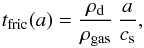 (6)where ρd is the dust material density, and ρgas is the gas density. We adopt ρdust = 3 g cm-3 and, from Fig. D.2, we get ρgas ≈ 10-15g cm-3 at r = 100 au.
Figure 9 shows that the observationally determined ΔX = 2 × 10⁻² is consistent with that predicted from a settled dust population whose vertically integrated size distribution is dn/ da = C·a-3.5, with a given amin. However, ΔX is currently likely much smaller, as we discuss below. While mm-to-cm grains have been directly detected in the inner disk of TW Hya, the disk is strongly depleted of millimetre-sized grains outside of 60 au (Wilner et al. 2005; Andrews et al. 2012). Thus, volatile loss onto large grains is likely not very efficient at r = 100 au at present, which implies that carbon was removed more efficiently in the past, that is Nmix< 200 and ΔX> 2 × 10⁻². Our results are consistent with amin ≳ 0.005 μm.
If the carbon loss happened on the same timescale as the loss of 1 cm grains due to radial migration – ttot ~ 105yr – we find ΔX = 0.9. The timescale for coagulation to 1 cm size – ttot ~ 106 yr – yields ΔX = 0.21. The dust growth timescale may be substantially shorter than this (e.g. Dullemond & Dominik 2005), in which case ΔX> 0.21 in the past.
The assumptions and predictions of our simple volatile loss model need to be tested with measurements of [C]/[H]gas in disks covering a range of ages and average temperatures, and we are pursuing such a follow-up programme. It is possible that grain growth provides an additional efficiency boost to the volatile loss process, by trapping some of the ices formed on small, coupled grains in larger particles via coagulation before the small grains can be mixed back to the disk surface (Du et al. 2015). The timescales of dust growth and vertical mixing are similar, within an order of magnitude, and their competition is not yet well observationally constrained. Direct measurements of the level of turbulence with ALMA show promise for remedying this (e.g. Hughes et al. 2011; Guilloteau et al. 2012; Flaherty et al. 2015).
6.3. The return of volatiles to the gas in the inner disk
Even around TW Hya, large ice-covered grains would eventually radially migrate close enough to the star for the volatiles to evaporate back to the gas phase. The current data do not allow us to robustly measure gas-phase elemental abundances in the inner disk for our targets to directly check this hypothesis. We propose to constrain the inner disk gas composition by studying the gas accreting onto the central stars.
Early-type stars, including Herbig Ae/Be stars, have radiative envelopes with mixing timescales that are longer than the timescale for accreting the mass of the stellar photosphere, and their observed photospheric abundances reflect the composition of the accreted material (Turcotte & Charbonneau 1993; Turcotte 2002). The photospheric abundances of Herbig Ae/Be stars were recently shown to be a predictor of the inner disk gas and dust content (Kama et al. 2015). This is in contrast to T Tauri stars, which have convective envelopes, where mixing rapidly erases accretion signatures.
Using tested stellar abundance analysis methods for Herbig stars (e.g. Folsom et al. 2012), we have derived the stellar abundances for HD 100546 (see Appendix A for a full description). HD 100546 displays the λ Boötis phenomenon, meaning it has approximately solar C, N and O abundances but is strongly depleted in refractory elements such as Fe, Si, Mg and Al. The λ Boö phenomenon is thought to be due to the preferential accretion of gas rather than dust (Venn & Lambert 1990). Intriguingly, Grady et al. (1997) inferred a relative enhancement of the C/Fe ratio in gas clouds accreting onto HD 100546. They further found siderophile elements overall to be depleted in the accreting gas. The above results are consistent with most C being in the gas phase in this disk, and thus being readily accreted onto the star. It also confirms that abundance ratios in the accretion flows do trace the composition of the accreting material.
Photospheric abundances for T Tauri stars are less sensitive to the composition of the currently accreting material, as noted above. Thus the stellar abundances for TW Hya would not reflect the inner disk composition. The connection between photospheric abundances and those in the accreting gas around HD 100546 suggests a way around this limitation, if the composition of the gas accreting onto TW Hya can be determined.
Studies of the UV spectrum of gas accreting onto TW Hya have found the [C iv]/[Si iv] ratio to be about an order of magnitude higher than in most other T Tauri stars, possibly owing to the accretion of silicon-poor (carbon-rich) material (e.g. Ardila et al. 2002; Herczeg et al. 2002; Ardila et al. 2013). This appears inconsistent with [C]/[H]gas= 10-6 and points to the sublimation of carbonaceous species in the inner disk. For the refractory silicates to not be accreted, they must remain trapped between the dust sublimation radius (close to the stellar surface for TW Hya) and the radius at which the carbon-rich ices evaporate (≲ 30 au for CO, ≲ 4 au for CH4). This implies an ongoing build-up of volatile-poor large dust particles or planetesimals within 30 au at most.
C2H2 and H2O were not detected in Spitzer/IRS mid-infrared spectroscopy of TW Hya by Najita et al. (2010). These observations probe the inner few astronomical units, much further out than the few stellar radii probed by UV observations of accreting gas. The mentioned species are commonly seen in such spectra and may originate from sublimation of ices or from gas-phase production mechanisms (e.g. Pascucci et al. 2009, 2013; Walsh et al. 2015). Their non-detection may indicate that the dust as well as the gas are depleted in the inner disk, and does not necessarily mean that the volatiles have not evaporated at all. Such inner disk depletions, with dust orders of magnitude more deficient than gas, have been found in ALMA studies of several transitional disks around Herbig Ae/Be stars (e.g. Bruderer et al. 2014; Zhang et al. 2014; van der Marel et al. 2015), and no doubt high spatial resolution observations of TW Hya will soon shed more light on the matter.
7. Conclusions
Based on new detections of atomic carbon emission from the disks around HD 100546 and TW Hya, we have revisited the gas-phase carbon abundance in the atmospheres of these disks. The analysis makes use of the DALI code and a range of continuum and spectral line data from the literature. For HD 100546, we also studied the stellar photospheric abundances, and for both systems employed various UV/NIR constraints to discuss elemental abundances in the inner disk.
-
1.
We present the first unambiguous detections of atomic carbon emission from protoplanetary disks, in the sources HD 100546 and TW Hya.
-
2.
For both disks, we fitted fully parametric physical models to the spectral energy distribution, spatially resolved CO emission, and a range of far-infrared emission lines. The most important difference from past physical models is that spatially resolved CO line emission is also reproduced.
-
3.
We confirm earlier findings that the HD 100546 disk atmosphere has either an interstellar gas-phase carbon abundance ([C]/[H]gas ≈ 10-4, if Δgas / dust = 10) or is moderately depleted ([C]/[H]gas≈ 10-5, if Δgas / dust = 100); and that the TW Hya disk atmosphere is two orders of magnitude deficient in gas-phase volatiles ([C]/[H]gas≈ 10-6, [O]/[H]gas≈ 10-6, and C / O > 1).
-
4.
Upper limits on HD emission for HD 100546 put an upper limit of 300 on the gas to dust ratio in the disk.
-
5.
The star HD 100546 has solar-like photospheric abundances of volatile elements (C, N, O) but a strong depletion of rock-forming elements (e.g. Fe, Mg, Si).
-
6.
Most carbon atoms in the HD 100546 disk gas have not passed through a hydrocarbon more complex than CH4 during the lifetime of the system.
-
7.
An underabundance of volatile elements in the disk atmosphere can develop when gas is mixed through the midplane and the temperature there allows freeze-out of major carrier species onto settled grains. An analytical formulation of this process is presented in Sect. 6.2.
-
8.
The volatiles return to the gas in the inner disk, as evidenced by their enhanced abundance relative to refractory elements in the gas accreting onto both stars.
Acknowledgments
We thank Catherine Walsh for sharing her ALMA data on HD 100546; Steve Doty and Sebastiaan Krijt for stimulating discussions; Sean Andrews and Gijs Mulders for sharing their compiled spectral energy distributions; and the ALLEGRO ALMA node in Leiden for their help. This work is supported by a Royal Netherlands Academy of Arts and Sciences (KNAW) professor prize, by the Netherlands Research School for Astronomy (NOVA), and by the European Union A-ERC grant 291141 CHEMPLAN. CPF acknowledges support from the French ANR grant “Toupies: Towards understanding the spin evolution of stars”. D.F. acknowledges support from the Italian Ministry of Education, Universities and Research project SIR (RBSI14ZRHR). This publication is based on data acquired with the Atacama Pathfinder Experiment (APEX), proposals 093.C-0926 and 093.F-0015, and on observations made with ESO telescopes at the La Silla Observatory under programme IDs 077.D-0092, 084.A-9016, and 085.A-9027. APEX is a collaboration between the Max-Planck-Institut für Radioastronomie, the European Southern Observatory, and the Onsala Space Observatory. This paper makes use of the following ALMA data: ADS/JAO.ALMA#2011.0.00863.S and ADS/JAO.ALMA#2011.0.00001.SV. ALMA is a partnership of ESO (representing its member states), NSF (USA) and NINS (Japan), together with NRC (Canada) and NSC and ASIAA (Taiwan), in cooperation with the Republic of Chile. The Joint ALMA Observatory is operated by ESO, AUI/NRAO, and NAOJ.
References
- Acke, B., & Waelkens, C. 2004, A&A, 427, 1009 [NASA ADS] [CrossRef] [EDP Sciences] [Google Scholar]
- Aikawa, Y., Umebayashi, T., Nakano, T., & Miyama, S. M. 1999, ApJ, 519, 705 [NASA ADS] [CrossRef] [Google Scholar]
- Akeson, R. L., Millan-Gabet, R., Ciardi, D. R., et al. 2011, ApJ, 728, 96 [NASA ADS] [CrossRef] [Google Scholar]
- Akiyama, E., Muto, T., Kusakabe, N., et al. 2015, ApJ, 802, L17 [NASA ADS] [CrossRef] [Google Scholar]
- Andrews, S. M., Wilner, D. J., Hughes, A. M., et al. 2012, ApJ, 744, 162 [NASA ADS] [CrossRef] [Google Scholar]
- Ardila, D. R., Basri, G., Walter, F. M., Valenti, J. A., & Johns-Krull, C. M. 2002, ApJ, 566, 1100 [NASA ADS] [CrossRef] [Google Scholar]
- Ardila, D. R., Golimowski, D. A., Krist, J. E., et al. 2007, ApJ, 665, 512 [NASA ADS] [CrossRef] [Google Scholar]
- Ardila, D. R., Herczeg, G. J., Gregory, S. G., et al. 2013, ApJS, 207, 1 [NASA ADS] [CrossRef] [EDP Sciences] [Google Scholar]
- Asplund, M., Grevesse, N., Sauval, A. J., & Scott, P. 2009, ARA&A, 47, 481 [NASA ADS] [CrossRef] [Google Scholar]
- Augereau, J. C., Lagrange, A. M., Mouillet, D., & Ménard, F. 2001, A&A, 365, 78 [NASA ADS] [CrossRef] [EDP Sciences] [Google Scholar]
- Balona, L. A. 1994, MNRAS, 268, 119 [NASA ADS] [CrossRef] [Google Scholar]
- Batalha, C., Batalha, N. M., Alencar, S. H. P., Lopes, D. F., & Duarte, E. S. 2002, ApJ, 580, 343 [NASA ADS] [CrossRef] [Google Scholar]
- Benisty, M., Tatulli, E., Ménard, F., & Swain, M. R. 2010, A&A, 511, A75 [NASA ADS] [CrossRef] [EDP Sciences] [Google Scholar]
- Bergin, E. A., Cleeves, L. I., Gorti, U., et al. 2013, Nature, 493, 644 [NASA ADS] [CrossRef] [PubMed] [Google Scholar]
- Bergin, E. A., Cleeves, L. I., Crockett, N., & Blake, G. A. 2014, Faraday Discuss., 168 [Google Scholar]
- Bouwman, J., de Koter, A., Dominik, C., & Waters, L. B. F. M. 2003, A&A, 401, 577 [NASA ADS] [CrossRef] [EDP Sciences] [Google Scholar]
- Brickhouse, N. S., Cranmer, S. R., Dupree, A. K., Luna, G. J. M., & Wolk, S. 2010, ApJ, 710, 1835 [NASA ADS] [CrossRef] [Google Scholar]
- Bruderer, S. 2013, A&A, 559, A46 [NASA ADS] [CrossRef] [EDP Sciences] [Google Scholar]
- Bruderer, S., Doty, S. D., & Benz, A. O. 2009, ApJS, 183, 179 [NASA ADS] [CrossRef] [Google Scholar]
- Bruderer, S., van Dishoeck, E. F., Doty, S. D., & Herczeg, G. J. 2012, A&A, 541, A91 [NASA ADS] [CrossRef] [EDP Sciences] [Google Scholar]
- Bruderer, S., van der Marel, N., van Dishoeck, E. F., & van Kempen, T. A. 2014, A&A, 562, A26 [NASA ADS] [CrossRef] [EDP Sciences] [Google Scholar]
- Calvet, N., D’Alessio, P., Hartmann, L., et al. 2002, ApJ, 568, 1008 [NASA ADS] [CrossRef] [Google Scholar]
- Cardelli, J. A., Meyer, D. M., Jura, M., & Savage, B. D. 1996, ApJ, 467, 334 [NASA ADS] [CrossRef] [Google Scholar]
- Cernicharo, J. 2004, ApJ, 608, L41 [NASA ADS] [CrossRef] [Google Scholar]
- Chabrier, G., Johansen, A., Janson, M., & Rafikov, R. 2014, Protostars and Planets VI, 619 [Google Scholar]
- Chapillon, E., Guilloteau, S., Dutrey, A., & Piétu, V. 2008, A&A, 488, 565 [NASA ADS] [CrossRef] [EDP Sciences] [Google Scholar]
- Chapillon, E., Parise, B., Guilloteau, S., Dutrey, A., & Wakelam, V. 2010, A&A, 520, A61 [NASA ADS] [CrossRef] [EDP Sciences] [Google Scholar]
- Chickos, J. S., Annuziata, R., Ladon, L. H., Hyman, A. S., & Liebman, J. F. 1986, J. Organic Chem., 51, 4311 [CrossRef] [Google Scholar]
- Cleeves, L. I., Bergin, E. A., Qi, C., Adams, F. C., & Öberg, K. I. 2015, ApJ, 799, 204 [NASA ADS] [CrossRef] [Google Scholar]
- de la Reza, R., Jilinski, E., & Ortega, V. G. 2006, AJ, 131, 2609 [NASA ADS] [CrossRef] [Google Scholar]
- Debes, J. H., Jang-Condell, H., Weinberger, A. J., Roberge, A., & Schneider, G. 2013, ApJ, 771, 45 [NASA ADS] [CrossRef] [Google Scholar]
- Dent, W. R. F., Thi, W. F., Kamp, I., et al. 2013, PASP, 125, 477 [NASA ADS] [CrossRef] [Google Scholar]
- Du, F., Bergin, E. A., & Hogerheijde, M. R. 2015, ApJ, 807, L32 [NASA ADS] [CrossRef] [Google Scholar]
- Dullemond, C. P., & Dominik, C. 2005, A&A, 434, 971 [NASA ADS] [CrossRef] [EDP Sciences] [Google Scholar]
- Dutrey, A., Guilloteau, S., Duvert, G., et al. 1996, A&A, 309, 493 [NASA ADS] [Google Scholar]
- Dutrey, A., Guilloteau, S., & Guelin, M. 1997, A&A, 317, L55 [NASA ADS] [Google Scholar]
- Dutrey, A., Guilloteau, S., & Simon, M. 2003, A&A, 402, 1003 [NASA ADS] [CrossRef] [EDP Sciences] [Google Scholar]
- Eisner, J. A., Chiang, E. I., & Hillenbrand, L. A. 2006, ApJ, 637, L133 [NASA ADS] [CrossRef] [Google Scholar]
- Favre, C., Cleeves, L. I., Bergin, E. A., Qi, C., & Blake, G. A. 2013, ApJ, 776, L38 [NASA ADS] [CrossRef] [Google Scholar]
- Fedele, D., Bruderer, S., van Dishoeck, E. F., et al. 2013a, A&A, 559, A77 [NASA ADS] [CrossRef] [EDP Sciences] [Google Scholar]
- Fedele, D., Bruderer, S., van Dishoeck, E. F., et al. 2013b, ApJ, 776, L3 [NASA ADS] [CrossRef] [Google Scholar]
- Fedele, D., van Dishoek, E. F., Kama, M., Bruderer, S., & Hogerheijde, M. R. 2016, A&A, 591, A95 [NASA ADS] [CrossRef] [EDP Sciences] [Google Scholar]
- Flaherty, K. M., Hughes, A. M., Rosenfeld, K. A., et al. 2015, ApJ, 813, 99 [NASA ADS] [CrossRef] [Google Scholar]
- Folsom, C. P., Bagnulo, S., Wade, G. A., et al. 2012, MNRAS, 422, 2072 [NASA ADS] [CrossRef] [MathSciNet] [Google Scholar]
- France, K., Schindhelm, E., Bergin, E. A., Roueff, E., & Abgrall, H. 2014, ApJ, 784, 127 [NASA ADS] [CrossRef] [Google Scholar]
- Furuya, K., & Aikawa, Y. 2014, ApJ, 790, 97 [NASA ADS] [CrossRef] [Google Scholar]
- Furuya, K., Aikawa, Y., Nomura, H., Hersant, F., & Wakelam, V. 2013, ApJ, 779, 11 [NASA ADS] [CrossRef] [Google Scholar]
- Gorti, U., Hollenbach, D., Najita, J., & Pascucci, I. 2011, ApJ, 735, 90 [NASA ADS] [CrossRef] [Google Scholar]
- Grady, C. A., Sitko, M. L., Bjorkman, K. S., et al. 1997, ApJ, 483, 449 [NASA ADS] [CrossRef] [Google Scholar]
- Grady, C. A., Polomski, E. F., Henning, T., et al. 2001, AJ, 122, 3396 [NASA ADS] [CrossRef] [Google Scholar]
- Guilloteau, S., Dutrey, A., Wakelam, V., et al. 2012, A&A, 548, A70 [NASA ADS] [CrossRef] [EDP Sciences] [Google Scholar]
- Güsten, R., Nyman, L. Å., Schilke, P., et al. 2006, A&A, 454, L13 [NASA ADS] [CrossRef] [EDP Sciences] [Google Scholar]
- Henning, T., Burkert, A., Launhardt, R., Leinert, C., & Stecklum, B. 1998, A&A, 336, 565 [NASA ADS] [Google Scholar]
- Herczeg, G. J., Linsky, J. L., Valenti, J. A., Johns-Krull, C. M., & Wood, B. E. 2002, ApJ, 572, 310 [NASA ADS] [CrossRef] [Google Scholar]
- Heyminck, S., Kasemann, C., Güsten, R., de Lange, G., & Graf, U. U. 2006, A&A, 454, L21 [NASA ADS] [CrossRef] [EDP Sciences] [Google Scholar]
- Hoff, W., Henning, T., & Pfau, W. 1998, A&A, 336, 242 [NASA ADS] [Google Scholar]
- Hogerheijde, M. R., Bergin, E. A., Brinch, C., et al. 2011, Science, 334, 338 [NASA ADS] [CrossRef] [PubMed] [Google Scholar]
- Hughes, A. M., Wilner, D. J., Andrews, S. M., Qi, C., & Hogerheijde, M. R. 2011, ApJ, 727, 85 [NASA ADS] [CrossRef] [Google Scholar]
- Hughes, A. M., Wilner, D. J., Calvet, N., et al. 2007, ApJ, 664, 536 [NASA ADS] [CrossRef] [Google Scholar]
- Kama, M., Folsom, C. P., & Pinilla, P. 2015, A&A, 582, L10 [NASA ADS] [CrossRef] [EDP Sciences] [Google Scholar]
- Kama, M., Bruderer, S., Carney, M., et al. 2016, A&A, 588, A108 [NASA ADS] [CrossRef] [EDP Sciences] [Google Scholar]
- Kamp, I., Thi, W.-F., Meeus, G., et al. 2013, A&A, 559, A24 [NASA ADS] [CrossRef] [EDP Sciences] [Google Scholar]
- Kastner, J. H., Huenemoerder, D. P., Schulz, N. S., Canizares, C. R., & Weintraub, D. A. 2002, ApJ, 567, 434 [NASA ADS] [CrossRef] [Google Scholar]
- Kastner, J. H., Hily-Blant, P., Rodriguez, D. R., Punzi, K., & Forveille, T. 2014, ApJ, 793, 55 [NASA ADS] [CrossRef] [Google Scholar]
- Kastner, J. H., Qi, C., Gorti, U., et al. 2015, ApJ, 806, 75 [NASA ADS] [CrossRef] [Google Scholar]
- Kaufer, A., Stahl, O., Tubbesing, S., et al. 1999, The Messenger, 95, 8 [Google Scholar]
- Kenyon, S. J., & Hartmann, L. 1995, ApJS, 101, 117 [NASA ADS] [CrossRef] [Google Scholar]
- Kupka, F., Piskunov, N., Ryabchikova, T. A., Stempels, H. C., & Weiss, W. W. 1999, A&AS, 138, 119 [NASA ADS] [CrossRef] [EDP Sciences] [MathSciNet] [PubMed] [Google Scholar]
- Kurucz, R. 1993, CDROM Model Distribution, Smithsonian Astrophys. Obs. [Google Scholar]
- Landstreet, J. D. 1988, ApJ, 326, 967 [NASA ADS] [CrossRef] [Google Scholar]
- Lee, J.-E., Bergin, E. A., & Nomura, H. 2010, ApJ, 710, L21 [NASA ADS] [CrossRef] [Google Scholar]
- Meeus, G., Montesinos, B., Mendigutía, I., et al. 2012, A&A, 544, A78 [NASA ADS] [CrossRef] [EDP Sciences] [Google Scholar]
- Meeus, G., Salyk, C., Bruderer, S., et al. 2013, A&A, 559, A84 [NASA ADS] [CrossRef] [EDP Sciences] [Google Scholar]
- Mermilliod, J.-C., Mermilliod, M., & Hauck, B. 1997, A&AS, 124, 349 [NASA ADS] [CrossRef] [EDP Sciences] [Google Scholar]
- Miotello, A., Bruderer, S., & van Dishoeck, E. F. 2014, A&A, 572, A96 [NASA ADS] [CrossRef] [EDP Sciences] [Google Scholar]
- Muders, D., Hafok, H., Wyrowski, F., et al. 2006, A&A, 454, L25 [NASA ADS] [CrossRef] [EDP Sciences] [Google Scholar]
- Mulders, G. D., Waters, L. B. F. M., Dominik, C., et al. 2011, A&A, 531, A93 [NASA ADS] [CrossRef] [EDP Sciences] [Google Scholar]
- Mulders, G. D., Min, M., Dominik, C., Debes, J. H., & Schneider, G. 2013, A&A, 549, A112 [NASA ADS] [CrossRef] [EDP Sciences] [Google Scholar]
- Muzerolle, J., Calvet, N., Briceño, C., Hartmann, L., & Hillenbrand, L. 2000, ApJ, 535, L47 [NASA ADS] [CrossRef] [PubMed] [Google Scholar]
- Najita, J. R., Carr, J. S., Strom, S. E., et al. 2010, ApJ, 712, 274 [NASA ADS] [CrossRef] [Google Scholar]
- Öberg, K. I., Murray-Clay, R., & Bergin, E. A. 2011, ApJ, 743, L16 [NASA ADS] [CrossRef] [Google Scholar]
- Panić, O., & Hogerheijde, M. R. 2009, A&A, 508, 707 [NASA ADS] [CrossRef] [EDP Sciences] [Google Scholar]
- Panić, O., van Dishoeck, E. F., Hogerheijde, M. R., et al. 2010, A&A, 519, A110 [NASA ADS] [CrossRef] [EDP Sciences] [Google Scholar]
- Panić, O., Ratzka, T., Mulders, G. D., et al. 2014, A&A, 562, A101 [NASA ADS] [CrossRef] [EDP Sciences] [Google Scholar]
- Pantin, E., Waelkens, C., & Lagage, P. O. 2000, A&A, 361, L9 [NASA ADS] [Google Scholar]
- Parvathi, V. S., Sofia, U. J., Murthy, J., & Babu, B. R. S. 2012, ApJ, 760, 36 [NASA ADS] [CrossRef] [Google Scholar]
- Pascucci, I., Apai, D., Luhman, K., et al. 2009, ApJ, 696, 143 [NASA ADS] [CrossRef] [Google Scholar]
- Pascucci, I., Herczeg, G., Carr, J. S., & Bruderer, S. 2013, ApJ, 779, 178 [NASA ADS] [CrossRef] [Google Scholar]
- Pollack, J. B., Hubickyj, O., Bodenheimer, P., et al. 1996, Icarus, 124, 62 [NASA ADS] [CrossRef] [Google Scholar]
- Pontoppidan, K. M., Salyk, C., Bergin, E. A., et al. 2014, Protostars and Planets VI, 363 [Google Scholar]
- Qi, C., Öberg, K. I., Wilner, D. J., et al. 2013, Science, 341, 630 [NASA ADS] [CrossRef] [PubMed] [Google Scholar]
- Qi, C., Ho, P. T. P., Wilner, D. J., et al. 2004, ApJ, 616, L11 [NASA ADS] [CrossRef] [Google Scholar]
- Rosenfeld, K. A., Qi, C., Andrews, S. M., et al. 2012, ApJ, 757, 129 [NASA ADS] [CrossRef] [Google Scholar]
- Shakura, N. I., & Sunyaev, R. A. 1973, A&A, 24, 337 [NASA ADS] [Google Scholar]
- Siess, L., Dufour, E., & Forestini, M. 2000, A&A, 358, 593 [Google Scholar]
- Sturm, B., Bouwman, J., Henning, T., et al. 2010, A&A, 518, L129 [NASA ADS] [CrossRef] [EDP Sciences] [Google Scholar]
- Thi, W.-F., van Zadelhoff, G.-J., & van Dishoeck, E. F. 2004, A&A, 425, 955 [NASA ADS] [CrossRef] [EDP Sciences] [Google Scholar]
- Thi, W.-F., Mathews, G., Ménard, F., et al. 2010, A&A, 518, L125 [NASA ADS] [CrossRef] [EDP Sciences] [Google Scholar]
- Thi, W.-F., Ménard, F., Meeus, G., et al. 2011, A&A, 530, L2 [NASA ADS] [CrossRef] [EDP Sciences] [Google Scholar]
- Thiabaud, A., Marboeuf, U., Alibert, Y., Leya, I., & Mezger, K. 2015, A&A, 574, A138 [NASA ADS] [CrossRef] [EDP Sciences] [Google Scholar]
- Tognelli, E., Prada Moroni, P. G., & Degl’Innocenti, S. 2011, A&A, 533, A109 [NASA ADS] [CrossRef] [EDP Sciences] [Google Scholar]
- Tsukagoshi, T., Momose, M., Saito, M., et al. 2015, ApJ, 802, L7 [NASA ADS] [CrossRef] [Google Scholar]
- Turcotte, S. 2002, ApJ, 573, L129 [NASA ADS] [CrossRef] [Google Scholar]
- Turcotte, S., & Charbonneau, P. 1993, ApJ, 413, 376 [NASA ADS] [CrossRef] [Google Scholar]
- Unterborn, C. T., Kabbes, J. E., Pigott, J. S., Reaman, D. M., & Panero, W. R. 2014, ApJ, 793, 124 [NASA ADS] [CrossRef] [Google Scholar]
- Vacca, W. D., & Sandell, G. 2011, ApJ, 732, 8 [NASA ADS] [CrossRef] [Google Scholar]
- van den Ancker, M. E., The, P. S., Tjin A Djie, H. R. E., et al. 1997, A&A, 324, L33 [NASA ADS] [Google Scholar]
- van der Marel, N., van Dishoeck, E. F., Bruderer, S., Pérez, L., & Isella, A. 2015, A&A, 579, A106 [NASA ADS] [CrossRef] [EDP Sciences] [Google Scholar]
- van der Wiel, M. H. D., Naylor, D. A., Kamp, I., et al. 2014, MNRAS, 444, 3911 [NASA ADS] [CrossRef] [Google Scholar]
- van Dishoeck, E. F. 2008, in IAU Symp. 251, eds. S. Kwok, & S. Sanford, 3 [Google Scholar]
- van Dishoeck, E. F., Bergin, E. A., Lis, D. C., & Lunine, J. I. 2014, Protostars and Planets VI, 835 [Google Scholar]
- van Leeuwen, F. 2007, A&A, 474, 653 [NASA ADS] [CrossRef] [EDP Sciences] [Google Scholar]
- van Zadelhoff, G.-J., van Dishoeck, E. F., Thi, W.-F., & Blake, G. A. 2001, A&A, 377, 566 [NASA ADS] [CrossRef] [EDP Sciences] [Google Scholar]
- Venn, K. A., & Lambert, D. L. 1990, ApJ, 363, 234 [NASA ADS] [CrossRef] [Google Scholar]
- Wade, G. A., Bagnulo, S., Kochukhov, O., et al. 2001, A&A, 374, 265 [NASA ADS] [CrossRef] [EDP Sciences] [Google Scholar]
- Walsh, C., Juhász, A., Pinilla, P., et al. 2014a, ApJ, 791, L6 [NASA ADS] [CrossRef] [Google Scholar]
- Walsh, C., Millar, T. J., Nomura, H., et al. 2014b, A&A, 563, A33 [NASA ADS] [CrossRef] [EDP Sciences] [Google Scholar]
- Walsh, C., Nomura, H., & van Dishoeck, E. 2015, A&A, 582, A88 [NASA ADS] [CrossRef] [EDP Sciences] [Google Scholar]
- Webb, R. A., Zuckerman, B., Platais, I., et al. 1999, ApJ, 512, L63 [NASA ADS] [CrossRef] [Google Scholar]
- Willacy, K., Klahr, H. H., Millar, T. J., & Henning, T. 1998, A&A, 338, 995 [NASA ADS] [Google Scholar]
- Wilner, D. J., Bourke, T. L., Wright, C. M., et al. 2003, ApJ, 596, 597 [NASA ADS] [CrossRef] [Google Scholar]
- Wilner, D. J., D’Alessio, P., Calvet, N., Claussen, M. J., & Hartmann, L. 2005, ApJ, 626, L109 [NASA ADS] [CrossRef] [Google Scholar]
- Youdin, A. N., & Lithwick, Y. 2007, Icarus, 192, 588 [NASA ADS] [CrossRef] [Google Scholar]
- Zhang, K., Isella, A., Carpenter, J. M., & Blake, G. A. 2014, ApJ, 791, 42 [NASA ADS] [CrossRef] [Google Scholar]
Appendix A: HD 100546 photospheric abundances
Photospheric abundances derived for HD 100546.
The photospheric properties of HD 100546 were derived through directly fitting synthetic spectra to the optical spectrum of the star. This process gives a measurements of Teff, log (g), vsin(i), and chemical abundances. The synthetic spectra were calculated using the Zeeman spectrum synthesis program (Landstreet 1988; Wade et al. 2001), using model stellar atmospheres from ATLAS9 (Kurucz 1993), and atomic data from the Vienna Atomic Line Data Base (VALD; Kupka et al. 1999). The best-fit stellar parameters were derived using and automatic χ2 minimization routine, in which all parameters were fitted simultaneously (Folsom et al. 2012).
This fitting process was performed on none independent spectral windows (416−427, 440−460, 460−480, 490−510, 510−520, 520−540, 540−560, 620−650, and 710−750 nm). The final best fit parameters are the averages of the individual windows, and the uncertainties are the standard deviations. In cases where a chemical abundance for an element was derived in only three or fewer windows, the uncertainties were increased to account for the full window-to-window variation, as well as any potential uncertainties due to line blending and continuum normalization. Great care was taken to avoid any lines contaminated by emission. Weak emission infilling of lines was identified by looking for lines with variability between the observations, and lines with asymmetries or anomalous profile shapes. This fitting process is identical to that used by Folsom et al. (2012).
The results of this fitting process were checked for consistence against the Balmer line profiles, and a good agreement was found. However, Balmer lines were not used as the primary constraint on Teff or log (g), due to the uncertainties normalizing very broad lines in echelle spectra, and due to the emission in at least the core of the lines.
The stellar properties derived during the photospheric abundance analysis for HD 100546 are Teff = (10 390 ± 600) K and log (g) = (4.20 ± 0.30). The projected rotational velocity is vsin(i) = (64.9 ± 2.2) km s-1. Chemical abundances are presented in Table A.1. Microturbulence could not be well constrained for the star, although it is small (<2 km s-1), and so we assumed a value of 1 km s-1 which is typical for a Herbig Be star (e.g. Folsom et al. 2012). An error of 1 km s-1 in microturbulence would produce an error significantly less than 1σ in all our derived parameters. We find strong underabundances of iron-peak elements as well as Mg, Al, Si, Ca and Sc. However, we find abundances consistent with solar for the volatile elements He, C, N, and O. Chemically, this star appears to be a λ Boö star.
HD 100546 has parallax of (10.32 ± 0.43) mas (van Leeuwen 2007) and a V magnitude of 6.68 ± 0.03 (Mermilliod et al. 1997; van Leeuwen 2007). Using the bolometric correction of Balona (1994) with our Teff, an intrinsic colour from Kenyon & Hartmann (1995), and a standard reddening law (AV = 3.1 × E(B−V)), we find a luminosity of L⋆= (25 ± 7) L⊙. With our Teff, the luminosity implies a radius of (1.5 ± 0.3) R⊙. Putting the star on the H-R diagram and comparing to the evolutionary tracks of Siess et al. (2000), we find M⋆= (2.3 ± 0.2) M⊙. The H-R diagram position is consistent with the zero-age main-sequence (ZAMS) or the end of the pre main-sequence (PMS), implying an age > 6 Myr, consistent with the estimate of van den Ancker et al. (1997).
Appendix B: Checking for extended emission around HD 100546
A ≳1000 au scale scattered light halo is seen around HD 100546 (Grady et al. 2001; Ardila et al. 2007), and the [C ii] emission is single-peaked, also suggesting a compact or extended envelope (Fedele et al. 2013b). To determine the disk origin of the CO and [C i] lines observed in this study, we performed four additional pointings on the [C i] 1–0 and the CO 3–2 lines (not discussed at length in the paper). These were offset by ± 10′′ in the N-S direction, and by ± 5′′ in the E-W direction. The pointings are shown in Fig. B.1, and the resulting spectra are shown in Fig. B.2. Considering the red- (N-E) and blueshifted (S-W) sides of the disk, all the spectra are fully consistent with the entire flux originating in the disk. We have also checked that the total CO 3–2 line flux in our APEX data is the same as that recovered from the ALMA observation of Walsh et al. (2014a). In summary, we confirm that the [C i] 1–0 and CO 3–2 transitions have no off-source contribution and that the CO line asymmetry represents a real azimuthal asymmetry in the disk emission, rather than pointing offsets.
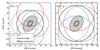 |
Fig. B.1 HD 100546 system. Black ellipses approximate the outer radius of CO 3−2 emission (solid line, Walsh et al. 2014a), μm-sized grains as traced by scattered light (dashed, Ardila et al. 2007), and the mm-sized grains as traced by the 860 μm continuum (dotted, Walsh et al. 2014a). The APEX pointings from this work are shown as coloured circles, corresponding directly to the spectra shown in Fig. B.2. |
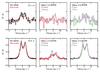 |
Fig. B.2 Observations of the [CI] 1−0 and CO 3−2 transitions towards HD 100546 and four nearby reference positions (offset by ± 5′′ East/West and ± 10′′ North/South, as shown in Fig. B.1). The emission strongly peaks at the disk and the red and blue peaks show variation expected from a Keplerian disk observed at the various offsets. |
Appendix C: Summary of observational data
In Table C.1, we list the line fluxes and upper limits used in the analysis. The SED for HD 100546 was adopted from Mulders et al. (2011, and references therein) and supplemented with ALMA measurements from Walsh et al. (2014a). The SED of TW Hya was adopted from Andrews et al. (2012, and references therein).
Line fluxes in units of 10-18W m-2.
Appendix D: Abundance and emission maps
In Figs. D.1 and D.2, we show the gas density, gas and dust temperature, and abundances of species relevant to this work in the HD 100546 and TW Hya disk. The main parameter in each panel is shown as a colourmap. The abundances are overlaid in black with the 25 and 75 % contours of the line contribution function. The contribution function represents the cumulative buildup of line emission, vertically integrated from top to bottom, and radially outward from the grid cell closest to the star at each height. The plotted contours show the area where both the vertical and radial cumulative emission contribution function for a given line is between 12.5 and 87.5 % (the 25 % contour), or between 37.5 and 62.5 % (the 75 % contour).
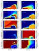 |
Fig. D.1 Disk structure and line contribution functions (CBFs) for the HD 100546 model with Δgas / dust = 10 and [C]/[H]gas= 1.35 × 10⁻⁴ (ISM). The CBF panels show the abundance (colour fill) and line emission (black lines) of CO, [C i], C2H, [C ii], and HD. The black contours encompass 25 and 75 % cumulative contributions to the line emission. The solid and dashed white lines show the τ = 1 surface for the line and continuum emission. The solid white line for Tgas and Tdust is the 50 K isotherm. |
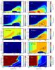 |
Fig. D.2 Disk structure and line contribution functions (CBFs) for the TW Hya model with Δgas / dust = 200 and [C]/[H]gas = 10-6 (depleted). The CBF panels show the abundance (colour fill) and line emission (black lines) of CO, [C i], C2H, [C ii], and HD. The black contours encompass 25 and 75% cumulative contributions to the line emission. The solid and dashed white lines show the τ = 1 surface for the line and continuum emission. The solid white lines for Tgas and Tdust are the 20 and 50 K isotherms. |
All Tables
Total and ultraviolet stellar luminosities for TW Hya and HD 100546 and a set of model stars with blackbody spectra.
All Figures
|
Fig. 1 [CI] 1−0 line in HD 100546 (offset by + 0.3 K) and TW Hya. Horizontal bars mark the systemic velocities, 5.70 and 2.86 km s-1. Red crosses show the best-fit Gaussian vlsr with 3σ error bars. The data are binned to 0.14 km s-1 per channel. |
| In the text | |
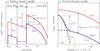 |
Fig. 2 Parametric disk structure used in DALI. See also Table 2. |
| In the text | |
|
Fig. 3 The ultraviolet range of spectra used in this study for TW Hya (red curve, France et al. 2014; Cleeves et al. 2015) and HD 100546 (blue curve, Bruderer et al. 2012), compared with blackbody photospheres for pre main sequence model stars with an age of 10 Myr (black curves, Tognelli et al. 2011). The two curves labelled 4000 K+UV show a 4000 K stellar photosphere with a 10 000 K blackbody added for the accretion rates Ṁ= 10-9 and 10-8 M⊙ yr-1. See also Table 3. |
| In the text | |
|
Fig. 4 Observations and modelling of HD 100546. The panels show, from top left to bottom, the spectral energy distribution; spectrally resolved line profiles; spatially resolved integrated CO 3–2 emission; and the full set of line fluxes used in the analysis. CO isotopolog lines for a given rotational transition are plotted at the same x-axis location. Two well-fitting models, with a gas to dust ratio Δgas / dust = 10 and [C]/[H]gas = 10-4 (solid blue) and Δgas / dust = 100 and [C]/[H]gas = 10-5 (dashed/open blue) are plotted on the observations (black) to illustrate the range of allowed parameters. The data and model values for C2H have been multiplied by a factor of 103 for display purposes. |
| In the text | |
|
Fig. 5 Observations and modelling of TW Hya. The panels show, from top left to bottom, the spectral energy distribution; spectrally resolved line profiles; spatially resolved integrated CO 3–2 emission; and the full set of line fluxes used in the analysis. CO isotopolog lines for a given rotational transition are plotted at the same x-axis location. Two well-fitting models, both with a gas to dust ratio Δgas / dust = 100 and [C]/[H]gas = 10-6 but with C/O = 0.47 (solid red) and 1.5 (dashed/open red) are plotted on the observations (black) to illustrate the range of allowed parameters. For C/O = 0.47, the [O i] 63 μm line model flux lies just above 10-16W m-2 and the C2H fluxes are a factor ≈ 103 below the observations. |
| In the text | |
|
Fig. 6 Gas-phase carbon abundance, compared with that of the Sun (dashed line, Asplund et al. 2009). From left to right: photospheric values for Herbig Ae/Be stars (Acke & Waelkens 2004; Folsom et al. 2012, stars); the stellar and disk values for HD 100546 (star and diamond, this work); the disk of TW Hya (diamond, this work); and lines of sight through the diffuse interstellar medium (Cardelli et al. 1996; Parvathi et al. 2012). For the Herbig Ae/Be and ISM samples, the median (black symbols) and the full dataset (small grey circles) are shown. |
| In the text | |
|
Fig. 7 Vertical structure of the TW Hya model at r = 100 au. Y denotes either the dust temperature (Tdust [K]), UV-field (G0), gas-phase CO and C0 abundance, or the grain size (a [μm]) of particles with a scaleheight hd equal to a given height z (see Eq. (5)). Vertical mixing can transport carbon atoms from the C0 layer to the freeze-out zone. |
| In the text | |
|
Fig. 8 Histograms of the fractional gas (solid lines) and dust mass (shaded) in 10 K temperature bins for the full disk of TW Hya (red) and HD 100546 (blue). Freeze-out temperatures of the main species for C and O loss from the gas to ices are marked with vertical dashed lines. |
| In the text | |
|
Fig. 9 Model of volatile loss from the disk atmosphere. Left-hand panel: a fraction ΔX of volatile atoms are lost in the midplane during each of Nmix mixing cycles. Equation (3) is shown for a depletion X0/X1 = 100 (solid curve). A theoretical turbulent mixing timescale gives Nmix = 200 (black dashed line) and ΔX = 2 × 10⁻² (dotted line), consistent with an upper limit of vturb ≤ 40 m s-1 on the speed of turbulent mixing in TW Hya, which gives Nmix ≤ 1300 (gray dashed line, Hughes et al. 2011). Right-hand panel: ΔX from Eq. (4), taking amax = 10 cm and amin = 0.001, 0.005, or 0.05 μm (solid lines). The smallest grain size settled below the CO freeze-out height at r = 100 au in our TW Hya model is also shown (dashed line, Eq. (5)). |
| In the text | |
|
Fig. B.1 HD 100546 system. Black ellipses approximate the outer radius of CO 3−2 emission (solid line, Walsh et al. 2014a), μm-sized grains as traced by scattered light (dashed, Ardila et al. 2007), and the mm-sized grains as traced by the 860 μm continuum (dotted, Walsh et al. 2014a). The APEX pointings from this work are shown as coloured circles, corresponding directly to the spectra shown in Fig. B.2. |
| In the text | |
|
Fig. B.2 Observations of the [CI] 1−0 and CO 3−2 transitions towards HD 100546 and four nearby reference positions (offset by ± 5′′ East/West and ± 10′′ North/South, as shown in Fig. B.1). The emission strongly peaks at the disk and the red and blue peaks show variation expected from a Keplerian disk observed at the various offsets. |
| In the text | |
|
Fig. D.1 Disk structure and line contribution functions (CBFs) for the HD 100546 model with Δgas / dust = 10 and [C]/[H]gas= 1.35 × 10⁻⁴ (ISM). The CBF panels show the abundance (colour fill) and line emission (black lines) of CO, [C i], C2H, [C ii], and HD. The black contours encompass 25 and 75 % cumulative contributions to the line emission. The solid and dashed white lines show the τ = 1 surface for the line and continuum emission. The solid white line for Tgas and Tdust is the 50 K isotherm. |
| In the text | |
|
Fig. D.2 Disk structure and line contribution functions (CBFs) for the TW Hya model with Δgas / dust = 200 and [C]/[H]gas = 10-6 (depleted). The CBF panels show the abundance (colour fill) and line emission (black lines) of CO, [C i], C2H, [C ii], and HD. The black contours encompass 25 and 75% cumulative contributions to the line emission. The solid and dashed white lines show the τ = 1 surface for the line and continuum emission. The solid white lines for Tgas and Tdust are the 20 and 50 K isotherms. |
| In the text | |
Current usage metrics show cumulative count of Article Views (full-text article views including HTML views, PDF and ePub downloads, according to the available data) and Abstracts Views on Vision4Press platform.
Data correspond to usage on the plateform after 2015. The current usage metrics is available 48-96 hours after online publication and is updated daily on week days.
Initial download of the metrics may take a while.