| Issue |
A&A
Volume 592, August 2016
|
|
|---|---|---|
| Article Number | A101 | |
| Number of page(s) | 12 | |
| Section | Cosmology (including clusters of galaxies) | |
| DOI | https://doi.org/10.1051/0004-6361/201526946 | |
| Published online | 08 August 2016 | |
Impacts of different SNLS3 light-curve fitters on cosmological consequences of interacting dark energy models
1 State Key Laboratory of Theoretical Physics, Institute of Theoretical Physics, Chinese Academy of Sciences, 100190 Beijing, PR China
e-mail: wangshuang@mail.sysu.edu.cn
2 Kavli Institute for Theoretical Physics China, Chinese Academy of Sciences, 100190 Beijing, PR China
3 School of Astronomy and Space Science, Sun Yat-Sen University, 510275 Guangzhou, PR China
Received: 12 July 2015
Accepted: 23 May 2016
We explore the cosmological consequences of interacting dark energy (IDE) models using the SNLS3 supernova samples. In particular, we focus on the impacts of different SNLS3 light-curve fitters (LCF; referred to in this paper as SALT2, SiFTO and combined sample). Firstly, making use of the three SNLS3 data sets, as well as the Planck distance priors data and the galaxy clustering data, we constrain the parameter spaces of three IDE models. Then, we study the cosmic evolutions of Hubble parameter H(z), deceleration diagram q(z), statefinder hierarchy S(1)3(z) and S(1)4(z), and check whether or not these dark energy diagnosis can distinguish the differences among the results of different SNLS3 LCF. Finally, we perform a high redshift cosmic age test using three old high redshift objects (OHRO), and explore the fate of the Universe. We find that the impacts of different SNLS3 LCF are rather small, and can not be distinguished using H(z), q(z), S(1)3(z), S(1)4(z), and the age data of OHRO. In addition, we infer, from the current observations, how far we are from a cosmic doomsday in the worst case, and find that the combined sample always gives the largest 2σ lower limit of the time interval between “big rip” and today, while the results given by the SALT2 and the SiFTO sample are similar. These conclusions are insensitive to a specific form of dark sector interaction. Our method can be used to distinguish the differences among various cosmological observations.
Key words: dark energy / cosmology: observations / cosmological parameters
© ESO, 2016
1. Introduction
Type Ia supernova is a sub-category of cataclysmic variable stars that results from the violent explosion of a white dwarf star in a binary system (Hillebrandt & Niemeyer 2000). Now it has become one of the most powerful probes to illuminate the mystery of cosmic acceleration (Riess et al. 1998; Perlmutter et al. 1999), which may be due to an unknown energy component that can produce an anti-gravitational effect, that is, dark energy (DE), or a modification of general relativity, that is, modified gravity (MG). (For recent reviews, we refer the reader to Frieman et al. 2008; Caldwell & Kamionkowski 2009; Uzan 2010; Wang 2010; Li et al. 2011a, 2013a; Weinberg et al. 2013.) Along with the rapid progress of supernova (SN) cosmology, several high quality SN datasets have been released in recent years, such as SNLS (Astier et al. 2006), union (Kowalski et al. 2008), constitution (Hicken et al. 2009), SDSS (Kessler et al. 2009), union2 (Amanullah et al. 2010), union2.1 (Suzuki et al. 2012), and pan-STARRS1 (Scolnic et al. 2014). In 2010, the supernova legacy survey (SNLS) group released their three-year data (Guy et al. 2010). Soon after, combining these SN samples with various low-z to mid-z samples and making use of three different light-curve fitters (LCF; an LCF is a method to model the light curves of SN; by using it one can estimate the distance information of each SN), Conley et al. presented three SNLS3 data sets (Conley et al. 2011): SALT2, which consists of 473 SN; SiFTO, which consists of 468 SN; and combined sample, which consists of 472 SN. It should be mentioned that, in the cosmology fits, the SNLS group treated two important quantities, stretch-luminosity parameter α and color-luminosity parameter β of SNe Ia, as free model parameters. We note that α and β are parameters for the luminosity standardization. In addition, the intrinsic scatter σint are fixed to ensure that χ2/ d.o.f. = 1.
A most critical challenge of SN cosmology is the control of the systematic uncertainties of type Ia supernovae (SNe Ia). One of the most important factors is the potential SN evolution. For example, previous studies on the union2.1 (Mohlabeng & Ralston 2014) and the pan-STARRS1 data sets (Scolnic et al. 2014) all indicated that β should evolve along with redshift z. Besides, it was found that the intrinsic scatter σint has the hint of redshift-dependence that will significantly affect the results of cosmology fits (Marriner et al. 2011). In addition to the SN evolution, another important factor is the choice of LCF (Kessler et al. 2009). For instance, it has been proved that even for the same SN samples, using MLCS2k2 (Jha et al. 2007) and SALT2 (Guy et al. 2007) LCF will lead to completely different fitting results for various cosmological models (Sollerman et al. 2009; Bueno Sanchez et al. 2009; Pigozzo et al. 2011; Smale & Wiltshire 2011; Bengochea 2011; Bengochea & De Rossi 2014).
One of the present authors has also done a series of research works to study the systematic uncertainties of SNe Ia. By using the SNLS3 dataset, we found that α is still consistent with a constant, but β evolves along with z at very high confidence level (CL) Wang & Wang (2013a). Soon after, we showed that this result has significant effects on the parameter estimation of standard cosmology (Wang et al. 2014a), and the introduction of a time-varying β can reduce the tension between SNe Ia and other cosmological observations. Moreover, we proved that our conclusion holds true for various DE and MG models (Wang et al. 2014b,c, 2015). Besides, the evolution of α has also been found for the JLA samples (Li et al. 2016). In addition, by using three different SNLS3 LCF, including SALT2, SiFTO and combined sample, we briefly discussed the effects of different LCF on the parameter estimation of the Λ-cold-dark-matter (ΛCDM) model Wang & Wang (2013a) and the holographic dark energy (HDE) model (Wang et al. 2015). It must be emphasized that in these two papers, only the fitting results given by different SNLS3 LCF are shown, and the corresponding cosmological consequences are not discussed. Therefore, the impacts of different LCF have not been studied in detail in our previous works. The main scientific objective of the current work is to present a comprehensive and systematic investigation on the impacts of different SNLS3 LCF. To do this, both the cosmology-fit results and the cosmological consequence results are shown in this work.
As mentioned above, the effects of different SNLS3 LCF on the ΛCDM model has been briefly discussed in Wang & Wang (2013a). To obtain new scientific results, new elements need to be taken into account. Since the interaction between different components widely exist in nature, and the introduction of a interaction between DE and CDM can provide an intriguing mechanism to solve the “cosmic coincidence problem” (Guo et al. 2007; Li et al. 2009b,a; He et al. 2010) and alleviate the “cosmic age problem” (Wang & Zhang 2008; Wang et al. 2010; Cui & Zhang 2010; Durán & Pavón 2011), it is interesting to study the effect of different LCF on interacting dark energy (IDE) model. Here we adopt the w-cold-dark-matter (wCDM) model with a direct non-gravitational interaction between dark sectors. We emphasize that, if our conclusions are dependent on the specific form of dark sector interaction, these conclusions will not be reliable at all. So in this work, three kinds of interaction terms are taken into account to ensure that our study is insensitive to a specific interaction form. In addition, to make a comparison, we also consider the case of wCDM model without an interaction term.
According to the previous studies on the potential SN evolution, we adopt a constant α and a linear β(z) = β0 + β1z in this work. Making use of the three SNLS3 data sets, as well as the latest Planck distance prior data (Wang & Wang 2013b), the galaxy clustering (GC) data extracted from Sloan digital sky survey (SDSS) data release 7 (DR7; Hemantha et al. 2014) and data release 9 (DR9; Wang 2014), we constrain the parameter spaces of the wCDM model and the three IDE models, and investigate the impacts of different SNLS3 LCF on the cosmology fits. Moreover, based on the fitting results, we study the possibility of distinguishing the impacts of different LCF by using various DE diagnosis tools and cosmic age data, and discuss the possible fate of the Universe.
We present our method in Sect. 2, our results in Sect. 3, and summarize and conclude in Sect. 4.
2. Methodology
In this section, firstly we review the theoretical framework of the IDE models, then we briefly describe the observational data used in the present work, and finally we introduce the background knowledge about DE diagnosis and cosmic age.
2.1. Theoretical models
This work is a sequel to the previous studies from our group, and thus we study the same IDE models considered in Wang et al. (2014b). It must be mentioned that here we consider a flat Universe and treat the present fractional density of radiation as a model parameter, which is a little different from the case of Wang et al. (2014b). The assumption of flatness is motivated by the inflation scenario. For a detailed discussion of the effects of spatial curvature, we refer reader to Clarkson et al. (2007). In a flat Universe, the Friedmann equation is 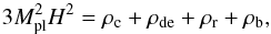 (1)where H ≡ ȧ/a is the Hubble parameter, a = (1 + z)-1 is the scale factor of the Universe (we take today’s scale factor a0 = 1), the dot denotes the derivative with respect to cosmic time t,
  is the reduced Planck mass, G is Newtonian gravitational constant, ρc, ρde, ρr and ρb are the energy densities of CDM, DE, radiation and baryon, respectively. The reduced Hubble parameter E(z) ≡ H(z) /H0 satisfies
 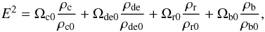 (2)where Ωc0, Ωde0, Ωr0 and Ωb0 are the present fractional densities of CDM, DE, radiation and baryon, respectively. As mentioned above, we treat Ωr0 as a model parameter in this work. In addition, ρr = ρr0(1 + z)4, ρb = ρb0(1 + z)3. Since Ωde0 = 1−Ωc0−Ωb0−Ωr0, Ωde0 is not an independent parameter.
In an IDE scenario, the energy conservation equations of CDM and DE satisfy 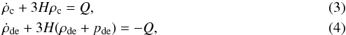 where pde = wρde is the pressure of DE, Q is the interaction term, which describes the energy transfer between CDM and DE. So far, the microscopic origin of interaction between dark sectors is still a puzzle. To study the issue of interaction, one needs to write down the possible forms of Q by hand. In this work we consider the following three cases:
 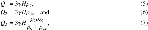 where γ is a dimensionless parameter describing the strength of interaction, γ> 0 means that energy transfers from DE to CDM, γ< 0 implies that energy transfers from CDM to DE, and γ = 0 denotes the case without dark sector interaction, that is, the wCDM model. We note that these three kinds of interaction form have been widely studied in the literature (Guo et al. 2007; Li et al. 2009a; He et al. 2010; Li & Zhang 2014). For simplicity, hereafter we call them IwCDM1 model, IwCDM2 model, and IwCDM3 model, respectively.
For the wCDM
model, we have  (8)For the IwCDM1 model, the solutions of Eqs. (3) and (4) are
  Then we have
  (11)For the IwCDM2 model, the solutions of Eqs. (3) and (4) are
  Then we get
  (14)For the IwCDM3 model, Eqs. (3) and (4) still have
analytical solutions
(14)For the IwCDM3 model, Eqs. (3) and (4) still have
analytical solutions  Then we obtain
  (17)where
  (18)For each model, the expression of E(z) will
be used to calculate the observational quantities appearing in the next subsection.
(18)For each model, the expression of E(z) will
be used to calculate the observational quantities appearing in the next subsection.
2.2. Observational data
In this subsection, we describe the observational data. Here we use the SNe Ia, CMB, and GC data, as we did in our previous paper (Wang et al. 2014a). It should be emphasized that, in this work we use all the three SNLS3 data sets (i.e., SALT2, SiFTO, and combined sample), while only the combined data are used in Wang et al. (2014a). In addition, the GC data are also updated in this work, compared to that used in Wang et al. (2014a).
2.2.1. SNe Ia data
As mentioned above, we use all the three SNLS3 data sets. In the following, we briefly introduce how to include these three data sets into the χ2 analysis.
Adopting a constant α and a linear β(z) = β0 + β1z, the predicted magnitude of an SN becomes  (19)The luminosity distance
  is defined as
  (20)where z and zhel are the CMB restframe and heliocentric redshifts of SN, and
 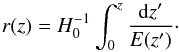 (21)Here s and
  are stretch measure and color measure for the SN light curve, ℳ is a parameter representing some combination of SN absolute magnitude M and Hubble constant H0.
For a set of N SNe with correlated errors, the χ2 function is given by 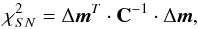 (22)where Δm ≡ mB−mmod is a vector with N components, and mB is the rest-frame peak B-band magnitude of the SN. The total covariance matrix C can be written as Conley et al. (2011)
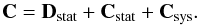 (23)Here Dstat denotes the diagonal part of the statistical uncertainty, Cstat and Csys denote the statistical and systematic covariance matrices, respectively. For the details of constructing the covariance matrix C, see Conley et al. (2011).
It must be emphasized that, in order to include host-galaxy information in the cosmological fits, Conley et al. split the SNLS3 sample based on host-galaxy stellar mass at 1010M⊙, and made ℳ to be different for the two samples Conley et al. (2011). So there are two values of ℳ (i.e., ℳ1 and ℳ2) for the SNLS3 data. Moreover, Conley et al. removed ℳ1 and ℳ2 from cosmology-fits by analytically marginalizing over them (for more details, see Appendix C of Conley et al. 2011). In the present work, we just follow the recipe of Conley et al. (2011), and do not treat ℳ as model parameter.
2.2.2. CMB data
For CMB data, we use the distance priors data extracted from Planck first data release (Wang & Wang 2013b). It should be mentioned that, in this paper we use the purely geometric measurements of CMB only, that is, the distance prior data. There are some other methods of using CMB data. For example, the observed position of the first peak of the CMB anisotropies spectrum can be used to perform cosmology-fits (Carneiro et al. 2008; Pigozzo et al. 2011). In addition, the CMB full data can also be used to constrain cosmological models via the global fit technique. To make a comparison, we constrain the parameter spaces of IwCDM1 model by using these three methods of using CMB data. We find that the differences among the fitting results given by different method are very small (e.g., the differences on DE EoS w are only in the order of 1%). In other words, Our results are insensitive to the method of using CMB data. This conclusion also holds true for other DE models (such as HDE model Li et al. 2013b), showing that the CMB data cannot put strict constraints on the properties of DE. Since the main purpose of using CMB data is to put strict constraints on Ωc0 and Ωb0, we think that the use of the Planck distance prior is sufficient enough for our work. CMB give us the comoving distance to the photon-decoupling surface r(z∗), and the comoving sound horizon at photon-decoupling epoch rs(z∗). It should be pointed out that, in this work, we adopt the result of z∗ given in (Hu & Sugiyama 1996). Wang and Mukherjee showed that the CMB shift parameters (Wang & Mukherjee 2007) 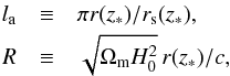 (24)together with ωb ≡ Ωbh2, provide an efficient summary of CMB data as far as dark energy constraints go. The comoving sound horizon is given by (Wang & Wang 2013b)
 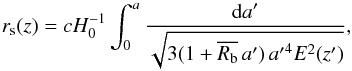 (25)where a is the scale factor of the Universe,
 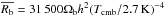 , and Tcmb = 2.7255 K.
Using the Planck+lensing+WP data, the mean values and 1σ errors of { la,R,ωb } are obtained (Wang & Wang 2013b): 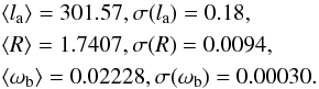 (26)Defining p1 = la(z∗), p2 = R(z∗), and p3 = ωb, the normalized covariance matrix NormCovCMB(pi,pj) can be written as (Wang & Wang 2013b)
 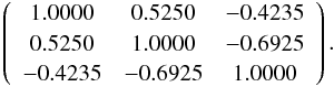 (27)Then, the covariance matrix for (la,R,ωb) is given by
  (28)where i,j = 1,2,3. The CMB data are included in our analysis by adding the following term to the χ2 function:
 ![\begin{equation} \label{eq:chi2CMB} \chi^2_{\rm CMB}=\Delta p_i \left[\mbox{Cov}^{-1}_{\rm CMB}(p_i,p_j)\right] \Delta p_j, \hskip .2cm \Delta p_i= p_i - p_i^{\rm data}, \end{equation}](/articles/aa/full_html/2016/08/aa26946-15/aa26946-15-eq95.png) (29)where
(29)where  are the mean values from Eq. (26).
2.2.3. GC data
To improve the cosmological constraints, we also use the GC data extracted from SDSS samples. Chuang & Wang (2013) measured the Hubble parameter H(z) and the angular-diameter distance DA(z) separately. Here, the angular-diameter distance 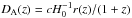 , where c is the speed of light. by scaling the model galaxy two-point correlation function to match the observed galaxy two-point correlation function. Since the scaling is measured by marginalizing over the shape of the model correlation function, the measured H(z) and DA(z) are model-independent and can be used to constrain any cosmological model (Chuang & Wang 2013).
It should be mentioned that, compared with using H(z) and DA(z), using H(z)rs(zd) /c and DA(z) /rs(zd) can give better constraints on various cosmological models. Here, rs(zd) is the sound horizon at the drag epoch, where rs(z) is given by Eq. (25), zd is given in Eisenstein & Hu (1998). In Hemantha et al. (2014), using the two-dimensional matter power spectrum of SDSS DR7 samples, Hemantha, Wang, and Chuang got  (30)In a similar work (Wang 2014), using the anisotropic two-dimensional galaxy correlation function of SDSS DR9 samples, Wang obtained
 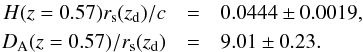 (31)GC data are included in our analysis by adding
  , with zGC1 = 0.35 and zGC2 = 0.57, to the χ2 of a given model. We note that
 ![\begin{equation} \label{eq:chi2bao} \chi^2_{\rm GCi}=\Delta q_i \left[{\rm C}^{-1}_{\rm GCi}(q_i,q_j)\right] \Delta q_j, \hskip .2cm \Delta q_i= q_i - q_i^{\rm data}, \end{equation}](/articles/aa/full_html/2016/08/aa26946-15/aa26946-15-eq110.png) (32)where q1 = H(zGCi)rs(zd) /c, q2 = DA(zGCi) /rs(zd), and i = 1,2. Based on Hemantha et al. (2014) and Wang (2014), we have
(32)where q1 = H(zGCi)rs(zd) /c, q2 = DA(zGCi) /rs(zd), and i = 1,2. Based on Hemantha et al. (2014) and Wang (2014), we have 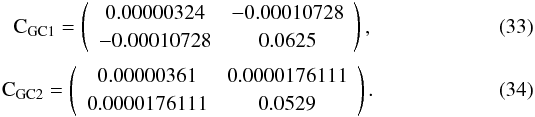
2.2.4. Total χ2 function
Now the total χ2 function is 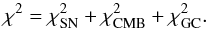 (35)We perform a Markov chain Monte Carlo likelihood analysis using the cosmoMC package (Lewis & Bridle 2002).
2.3. Dark energy diagnosis and cosmic age
Since previous works pointed out that the differences among the cosmological results given by the three different SNLS3 LCF are rather small, we need more tools to distinguish the effects of different LCF. In the present work, we use the Hubble parameter H(z), the deceleration parameter q(z), the statefinder hierarchy  and
and  (Arabsalmani & Sahni 2011; Zhang et al. 2014), and the cosmic age t(z) as our diagnosis tools to distinguish the effects of different LCF. This subsection consists of two parts. Firstly, we introduce the tools of DE diagnosis, including the Hubble parameter H(z), the deceleration parameter q(z), and the statefinder hierarchy
  . Then, we discuss the issues of cosmic age, including the high-redshift cosmic age test and the fate of the Universe.
Let us introduce the DE diagnosis tools first. The scale factor of the Universe a can be Taylor expanded around today’s cosmic age t0 as follows: ![\begin{equation} a(t)=1+\sum\limits_{\emph{n}=1}^{\infty}\frac{A_{\emph{n}}}{n!}[H_0(t-t_0)]^n, \end{equation}](/articles/aa/full_html/2016/08/aa26946-15/aa26946-15-eq120.png) (36)where
(36)where 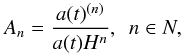 (37)with a(t)(n) = dna(t) / dtn. The Hubble parameter H(z) contains the information of the first derivative of a(t). Based on the Baryon acoustic oscillations (BAO) measurements from the SDSS data releases 9 and 11, Samushia et al. (2013) gave H0.57 ≡ H(z = 0.57) = 92.4 ± 4.5 km s-1 Mpc-1, while Delubac et al. (2015) obtained H2.34 ≡ H(z = 2.34) = 222 ± 7 km s-1 Mpc-1. These two H(z) data points will be used to compare the theoretical predictions of the wCDM model and the three IDE models. In addition, the deceleration parameter q is given by
 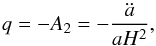 (38)which contains the information of the second derivatives of a(t). For the ΛCDM model,
  , A3 | ΛCDM = 1,
  . The statefinder hierarchy, Sn, is defined as (Arabsalmani & Sahni 2011):
 ![\begin{eqnarray} &&S_{2}=A_{2}+\frac{3}{2}\Omega_{\rm m},\\[2mm] &&S_{3}=A_{3},\\[2mm] &&S_{4}=A_{4}+\frac{3^2}{2}\Omega_{\rm m}. \end{eqnarray}](/articles/aa/full_html/2016/08/aa26946-15/aa26946-15-eq132.png) The reason for this redefinition is to peg the statefinder at unity for ΛCDM during the cosmic expansion,
The reason for this redefinition is to peg the statefinder at unity for ΛCDM during the cosmic expansion,  (42)This equation defines a series of null diagnostics for ΛCDM when n ≥ 3. By using this diagnostic, we can easily distinguish the ΛCDM model from other DE models. Because of
  , when n ≥ 3, statefinder hierarchy can be rewritten as:
 ![\begin{eqnarray} &&S^{(1)}_{3}=A_{3},\\[2mm] &&S^{(1)}_{4}=A_{4}+3(1+q), \end{eqnarray}](/articles/aa/full_html/2016/08/aa26946-15/aa26946-15-eq136.png) where the superscript (1) is to discriminate between
where the superscript (1) is to discriminate between  and Sn. In this paper, we use the statefinder hierarchy and as our diagnosis tools to distinguish the effects of different LCF.
Now, let us turn to the issue of cosmic age. The age of the Universe at redshift z is given by  (45)Historically, the cosmic age problem played an important role in cosmology (Alcaniz & Lima 1999; Lan et al. 2010; Bengaly et al. 2014; Liu & Zhang 2014). Obviously, the Universe cannot be younger than its constituents. In other words, the age of the Universe at any high redshift z cannot be younger than its constituents at the same redshift. There are some old high redshift objects (OHRO) considered extensively in the literature. For instance, the 3.5 Gyr old galaxy LBDS 53W091 at redshift z = 1.55 (Dunlop et al. 1996), the 4.0 Gyr old galaxy LBDS 53W069 at redshift z = 1.43 (Dunlop 1999), and the old quasar APM 08279+5255, whose age is estimated to be 2.0 Gyr, at redshift z = 3.91Hasinger et al. (2002). In the literature, the age data of these three OHRO (i.e., t1.43 ≡ t(z = 1.43) = 4.0 Gyr, t1.55 ≡ t(z = 1.55) = 3.5 Gyr and t3.91 ≡ t(z = 3.91) = 2.0 Gyr) have been extensively used to test various cosmological models (see e.g., Alcaniz et al. 2003; Wei & Zhang 2007; Wang & Zhang 2008; Wang et al. 2010; Yan et al. 2015). In the present work, we will use these three age data points to test the wCDM model and the three IDE models.
Another interesting topic is the fate of the Universe. The future of the Universe depends on the property of DE. If the Universe is dominated by a quintessence (Caldwell et al. 1998; Zlatev et al. 1999) or a cosmological constant, the expansion of the Universe will continue forever. If the Universe is dominated by a phantom (Caldwell 2002; Caldwell et al. 2003), eventually the repulsive gravity of DE will become large enough to tear apart all the structures, and the Universe will finally encounter a doomsday, that is the so-called big rip (BR). Setting x = −ln(1 + z), we can get the time interval between a BR and today 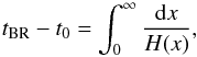 (46)where tBR denotes the time of the BR. It is obvious that, for a Universe dominated by a quintessence or a cosmological constant, this integration is infinity; and for a Universe dominated by a phantom, this integration is convergence. We would like to infer, from the current observational data, how far we are from a cosmic doomsday in the worst case. So in this work we calculate the 2σ lower limits of tBR−t0 for all the four DE models.
3. Results
In this section, firstly we show the cosmology-fit results of the wCDM model given by various SNLS3 samples without and with systematic uncertainties, next we present the fitting results of the three IDE models, then we show the cosmic evolutions of Hubble parameter H(z), deceleration parameter q(z), statefinder hierarchy and according to the fitting results of the IDE models, finally we perform the high-redshift cosmic age test and discuss the fate of the Universe. Since both three SNLS3 datasets and a time-varying β are considered at the same time, all the results of this work are new compared with the previous studies.
3.1. Cosmology fits
Fitting results for the wCDM model given by various SNLS3 samples without and with systematic uncertainties, where both the best-fit values and the 1σ errors of Ωm0 and w are listed.
In Table 1, we present the fitting results of the wCDM model given by various SNLS3 samples without and with systematic uncertainties. The first row of Table 1 shows the fitting results for the case of only considering constant β and statistical uncertainties. From this row we find that the best-fit values of Ωm0 and w given by the combined sample are in-between the best-fit results given by the SALT2 sample and by the SiFTO sample. This result is consistent with the result of Conley et al. (2011). The second row of Table 1 shows the fitting results for the case of considering constant β and statistical+systematic uncertainties. From this row we can see that, once the systematic uncertainties of SNLS3 samples are taken into account, the best-fit values of Ωm0 and w given by the combined sample are no longer between the best-fit results given by the SALT2 sample and by the SiFTO sample. Therefore, the reason for this strange phenomenon is the systematic uncertainties of SNLS3 samples. To further study this issue, in the third row of Table 1, we present the fitting results for the case of considering linear β and statistical+systematic uncertainties. We find that, after considering the evolution of β, the best-fit value of w given by the combined sample is in-between the results given by the SALT2 sample and by the SiFTO sample, while the differences among the best-fit values of Ωm0 given by the three SNLS3 samples are effectively reduced. These results imply the importance of considering β’s evolution in the cosmology-fits. Therefore, from now on we only consider the case of linear β.
Fitting results for the wCDM model and the three IDE models, where both the best-fit values and the 1σ errors of various parameters are listed.
In Table 2, by adopting a linear β, we give the fitting results of the wCDM model and the three IDE models. From this table we see that, for all the four DE models, β significantly deviates from a constant, consistent with the results of Wang et al. (2014b); in addition, there is no evidence for the existence of dark sector interaction. Although the best-fit results of w given by the three LCF are always less than −1, w = −1 is still consistent with the current cosmological observations at 2σ CL. Moreover, we check the impacts of different SNLS3 LCF on parameter estimation and find that for all the four DE models: (1) the combined sample always gives the largest w; in addition, the values of w given by the SALT2 and the SiFTO sample are close to each other. (2) The effects of different LCF on other parameters are negligible. It is clear that these results are insensitive to a specific DE model.
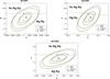 |
Fig. 1 Probability contours at the 1σ and 2σ CL in the γ–w plane, for the IwCDM1 (upper left panel), the IwCDM2 (upper right panel) and the IwCDM3 (lower panel) model. combined (black solid lines), SALT2 (red dashed lines), and SiFTO (green dash-dotted lines) denote the results given by the SN(combined)+CMB+GC, the SN(SALT2)+CMB+GC, and the SN(SiFTO)+CMB+GC data, respectively. Furthermore, the best-fit values of { γ,w } of the combined, SALT2 and the SiFTO data are marked as a black square, a red triangle and a green diamond, respectively. To make a comparison, the fixed point { γ,w } = { 0,−1 } for the ΛCDM model is also marked as a blue round dot. The gray solid line divides the panel into two regions: the region above the dividing line denotes a quintessence dominated Universe (without big rip), and the region below the dividing line represents a phantom dominated Universe (with big rip). |
In Fig. 1, we plot the probability contours at the 1σ and 2σ CL in the γ–w plane, for the three IDE models. A most obvious feature of this figure is that, for all the IDE models, the fixed point { 0,−1 } of the ΛCDM model is outside the 1σ contours given by the three data sets; however, the ΛCDM model is still consistent with the observational data at 2σ CL. Moreover, according to the evolution behaviors of ρde (see Eqs. (10), (12) and (16)) at z → −1, we divide these γ–w planes into two regions: the region above the dividing line denotes a quintessence dominated Universe (without big rip), and the region below the dividing line represents a phantom dominated Universe (with big rip). We can see that, although all the best-fit points given by the three data sets correspond to a phantom, both phantom, quintessence and cosmological constant are consistent with the current cosmological observations at 2σ CL. This means that the current observational data are still too limited to indicate the nature of DE.
3.2. Hubble parameter, deceleration parameter and statefinder hierarchy
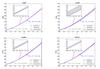 |
Fig. 2 The 1σ confidence regions of Hubble parameter H(z) at redshift region [0,4], for the wCDM (upper left panel), the IwCDM1 (upper right panel), the IwCDM2 (lower left panel), and the IwCDM3 (lower right panel) model, where the data points of H0.57 and H2.34 are also marked by diamonds with error bars for comparison. combined (gray filled regions), SALT2 (blue solid lines), and SiFTO (purple dashed lines) denote the results given by the SN(combined)+CMB+GC, the SN(SALT2)+CMB+GC, and the SN(SiFTO)+CMB+GC data, respectively. |
The 1σ confidence regions of Hubble parameter H(z) at redshift region [0,4] for the wCDM model and the three IDE models are plotted in Fig. 2, where the two H(z) data points, H0.57 and H2.34, are also marked by diamonds with error bars for comparison. We find that the data point H0.57 can be easily accommodated in the wCDM model and the three IDE models, but the data point H2.34 significantly deviates from the 1σ regions of all the four DE models. In other words, the measurement of H2.34 is in tension with other cosmological observations and this result is consistent with the conclusion of Sahni et al. (2014), Hu et al. (2014). In addition, the 1σ confidence regions of H(z) given by different LCF are almost overlap; this means that using H(z) diagram is almost impossible to distinguish the differences among different SNLS3 LCF.
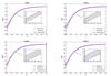 |
Fig. 3 The 1σ confidence regions of deceleration parameter q(z) at redshift region [0,4] for the wCDM (upper left panel), the IwCDM1 (upper right panel), the IwCDM2 (lower left panel) and the IwCDM3 (lower right panel) model. combined (gray filled regions), SALT2 (blue solid lines), and SiFTO (purple dashed lines) denote the results given by the SN(combined)+CMB+GC, the SN(SALT2)+CMB+GC, and the SN(SiFTO)+CMB+GC data, respectively. |
In Fig. 3, we plot the 1σ confidence regions of deceleration parameter q(z) at redshift region [0,4], for the wCDM model and the three IDE models. Again, we see that the 1σ confidence regions of q(z) given by different LCF are almost overlap. This implies that it is very difficut to distinguish the differences among different SNLS3 LCF using q(z) diagram.
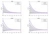 |
Fig. 4 The 1σ confidence regions of |
In Fig. 4, we plot the 1σ confidence regions of at redshift region [0,4], for the wCDM model and the three IDE models. From this figure we see that, the 1σ confidence regions of given by the three SNLS3 LCF almost overlap at high redshift. Although there is an separating trend for when z → 0, most parts of these three 1σ regions are overlap even at the current epoch. This means that, although is a better tool than H(z) and q(z), it still has difficulty distinguishing the effects of different SNLS3 LCF. Moreover, our conclusion holds true for all four DE models, showing that this conclusion is insensitive to a specific interaction form.
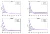 |
Fig. 5 The 1σ confidence regions of |
In Fig. 5, we plot the 1σ confidence regions of at redshift region [0,4], for the wCDM model and the three IDE models. From this figure we see that most of the 1σ confidence regions of given by the three LCF are overlap. This means that the effects of different LCF can not be distinguished by using the statefinder either. Again, we see that this conclusion is insensitive to a specific interaction form.
In conclusion, we find that the differences given by SALT2, SiFTO, and combined LCF are rather small and can not be distinguished using H(z), q(z), and . This result is quite different from the case of MLCS2k2 (Jha et al. 2007) and SALT2 (Guy et al. 2007), where using MLCS2k2 and SALT2 LCF gives completely different cosmological constraints for various models Bengochea (2011), Bengochea & De Rossi (2014).
3.3. Cosmic age and fate of the Universe
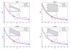 |
Fig. 6 The 2σ confidence regions of cosmic age t(z) at redshift region [0,4], for the wCDM (upper left panel), the IwCDM1 (upper right panel), the IwCDM2 (lower left panel) and the IwCDM3 (lower right panel) model. Three t(z) data points, t1.43, t1.55 and t3.91, are also marked by Squares for comparison. combined (gray filled regions), SALT2 (blue solid lines), and SiFTO (purple dashed lines) denote the results given by the SN(combined)+CMB+GC, the SN(SALT2)+CMB+GC, and the SN(SiFTO)+CMB+GC data, respectively. |
The 2σ confidence regions of cosmic age t(z) at redshift region [0,4] for the wCDM model and the three IDE models are plotted in Fig. 6, where the three t(z) data points, t1.43, t1.55 and t3.91, are also indicated for comparison. We find that both t1.43 and t1.55 can be easily accommodated in all the four DE models, but the position of t3.91 is significantly higher than the 2σ upper bounds of all the four DE models. In other words, the existence of the old quasar APM 08279+5255 still can not be explained in the frame of IDE model. This result is consistent with the conclusions of previous studies Alcaniz et al. (2003), Wei & Zhang (2007), Wang & Zhang (2008), Wang et al. (2008, 2010), Yan et al. (2015). In addition, the 2σ regions of t(z) given by different LCF almost overlap, showing that the impacts of different SNLS3 LCF can not be distinguished by using the age data of OHRO.
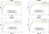 |
Fig. 7 The 2σ lower limits of the time interval t−t0 between a future moment and today, for the wCDM (upper left panel), the IwCDM1 (upper right panel), the IwCDM2 (lower left panel) and the IwCDM3 (lower right panel) model. combined (black solid lines), SALT2 (red dashed lines), and SiFTO (green dash-dotted lines) denote the results given by the SN(combined)+CMB+GC, the SN(SALT2)+CMB+GC, and the SN(SiFTO)+CMB+GC data, respectively. The 2σ lower bound values of tBR−t0 given by the three SNLS3 data are also listed on this figure. |
We want to infer how far we are from a cosmic doomsday in the worst case. So in Fig. 7, we plot the 2σ lower limits of the time interval t−t0 between a future moment and today, for the wCDM model and the three IDE models. Moreover, the 2σ lower limit values of tBR−t0 given by the three LCF are also marked on this figure. The 2σ upper limits of tBR−t0 is infinite; in other words, the Universe will expand eternally. All the evolution curves of t−t0 tend to the corresponding convergence values at −ln(1 + z) ≃ 20. The most important factor in determining tBR−t0 is the EoS w. In a phantom-dominated Universe, a smaller w corresponds to a larger increasing rate of ρde; this means that all the gravitationally bound structures will be torn apart in a shorter time, and the Universe will encounter a cosmic doomsday in a shorter time, too. Among the three SNLS3 LCF data, the combined sample always gives the largest w, and thus gives the largest value of tBR−t0. In addition, the values of w given by the SALT2 and the SiFTO sample are close to each other, and thus the values of tBR−t0 given by these two samples are close to each other.
4. Summary and discussion
As is well known, different LCF will yield different SN sample. In 2011, based on three different LCF, the SNLS3 group (Conley et al. 2011) released three kinds of SN samples, that is, SALT2, SiFTO and combined. So far, only the SNLS3 combined sample has been studied extensively, both the SALT2 and the SiFTO data sets are seldom taken into account in the literature. Moreover, the cosmological consequences given by these three SNLS3 LCF have not been discussed before. Therefore, the impacts of different SNLS3 LCF have not been studied in detail in the past. The main aim of the present work is to present a comprehensive and systematic investigation on the impacts of different SNLS3 LCF.
Since the interaction between different components widely exist in nature, and the introduction of a interaction between DE and CDM can provide an intriguing mechanism to solve the cosmic coincidence problem and alleviate the cosmic age problem, here we adopt the wCDM model with a dark sector interaction. To ensure that our study is insensitive to a specific dark sector interaction, three kinds of interaction terms are taken into account in this work. In addition, to make a comparison, we also consider the case of wCDM model without dark sector interaction.
We have used the three SNLS3 data sets, as well as the observational data from the CMB and the GC, to constrain the parameter spaces of the wCDM model and the three IDE models. According to the results of cosmology-fits, we have plotted the cosmic evolutions of Hubble parameter H(z), deceleration parameter q(z), statefinder hierarchy and , and have checked whether or not these DE diagnoses can distinguish the differences among the results of different LCF. Furthermore, we have performed high-redshift cosmic age test using three OHRO, and have explored the fate of the Universe.
We find that for the wCDM and all the three IDE models: (1) the combined sample always gives the largest w; in addition, the values of w given by the SALT2 and the SiFTO sample are similar. (see Table 2 and Fig. 1); (2) the effects of different SNLS3 LCF on other parameters are negligible (see Table 2). Besides, we find that the ΛCDM model is inconsistent with the three SNLS3 samples at 1σ CL, but is still consistent with the observational data at 2σ CL.
Moreover, we find that the impacts of different SNLS3 LCF are rather small and can not be distinguished by using H(z) (see Fig. 2), q(z) (see Fig. 3), (see Fig. 4), (see Fig. 5), and t(z) diagram (see Fig. 6). This result is quite different from the case of MLCS2k2 (Jha et al. 2007) and SALT2 (Guy et al. 2007), where using MLCS2k2 and SALT2 LCF will give completely different cosmological constraints for various models (Bengochea 2011; Bengochea & De Rossi 2014). In addition, we infer how far we are from a cosmic doomsday in the worst case, and find that the combined sample always gives the largest 2σ lower limit of tBR−t0, while the results given by the SALT2 and the SiFTO sample are similar (see Fig. 7).
Since the conclusions listed above hold true for all the three IDE models, we can conclude that the impacts of different SNLS3 LCF are insensitive to the specific forms of dark sector interaction. In addition, these conclusions also come into existence for the case of the wCDM model. Our method can be used to distinguish the differences among various cosmological observations (e.g., see Hu et al. 2015; Wang et al. 2016).
For simplicity, in the present work we only adopt a constant w, and do not consider the possible evolution of w. In the literature, the dynamical evolution of EoS are often explored by assuming a specific ansatz for w(z) (Chevallier & Polarski 2001; Linder 2003; Gerke & Efstathiou 2002; Wetterich 2004; Jassal et al. 2005), or by adopting a binned parametrization (Huterer & Starkman 2003; Huterer & Cooray 2005; Huang et al. 2009; Wang et al. 2011; Li et al. 2011b; Gong et al. 2013). To further study the impacts of various systematic uncertainties of SNe Ia on parameter estimation, we will extend our investigation to the case of a time-varying w in the future.
In a recent paper Betoule et al. (2014), based on the improved SALT2 LCF, Betoule et al presented a latest SN data set (joint light-curve analysis (JLA) data set), which consists of 740 SNe Ia. Adopting a constant α and a constant β, Betoule et al. found Ωm0 = 0.295 ± 0.034 for a flat ΛCDM model; this result is different from the result of SNLS3 data, but is consistent with the results of Planck (Planck Collaboration XVI 2014). It would be interesting to apply our method to compare the differences between the SNLS3 and the JLA sample. These issues will be studied in future works.
Acknowledgments
We are grateful to the referee for the valuable suggestions. We also thank Prof. Yun Wang, Prof. Anze Slosar, Prof. Xin Zhang and Dr. Yun-He Li for helpful discussions. S.W. is supported by the national natural science foundation of China under grant No. 11405024 and the fundamental research funds for the central universities (Grant No. N130305007 and grant No. 16lgpy50). M.L. is supported by the national natural science foundation of China (Grant No. 11275247, and grant No. 11335012) and a 985 grant at Sun Yat-Sen university.
References
- Alcaniz, J. S., & Lima, J. A. S. 1999, ApJ, 521, L87 [NASA ADS] [CrossRef] [Google Scholar]
- Alcaniz, J. S., Lima, J. A. S., & Cunha, J. V. 2003, MNRAS, 340, L39 [NASA ADS] [CrossRef] [Google Scholar]
- Amanullah, R., Lidman, C., Rubin, D., et al. 2010, ApJ, 716, 712 [NASA ADS] [CrossRef] [Google Scholar]
- Arabsalmani, M., & Sahni, V. 2011, Phys. Rev. D, 83, 043501 [NASA ADS] [CrossRef] [Google Scholar]
- Astier, P., Guy, J., Regnault, N., et al. 2006, A&A, 447, 31 [NASA ADS] [CrossRef] [EDP Sciences] [Google Scholar]
- Bengaly, C. A. P., Dantas, M. A., Carvalho, J. C., & Alcaniz, J. S. 2014, A&A, 561, A44 [NASA ADS] [CrossRef] [EDP Sciences] [Google Scholar]
- Bengochea, G. R. 2011, Phys. Lett. B, 696, 5 [NASA ADS] [CrossRef] [Google Scholar]
- Bengochea, G. R., & De Rossi, M. E. 2014, Phys. Lett. B, 733, 258 [NASA ADS] [CrossRef] [Google Scholar]
- Betoule, M., Kessler, R., Guy, J., et al. 2014, A&A, 568, A22 [NASA ADS] [CrossRef] [EDP Sciences] [Google Scholar]
- BuenoSanchez, J. C., Nesseris, S., & Perivolaropoulos, L. 2009, J. Cosmol. Astropart. Phys., 11, 029 [NASA ADS] [Google Scholar]
- Caldwell, R. R. 2002, Phys. Lett. B, 545, 23 [NASA ADS] [CrossRef] [Google Scholar]
- Caldwell, R. R., & Kamionkowski, M. 2009, Ann. Rev. Nucl. Part. Sci., 59, 397 [NASA ADS] [CrossRef] [Google Scholar]
- Caldwell, R. R., Dave, R., & Steinhardt, P. J. 1998, Phys. Rev. Lett., 80, 1582 [Google Scholar]
- Caldwell, R. R., Kamionkowski, M., & Weinberg, N. N. 2003, Phys. Rev. Lett., 91, 071301 [NASA ADS] [CrossRef] [PubMed] [Google Scholar]
- Carneiro, S., Dantas, M. A., Pigozzo, C., & Alcaniz, J. S. 2008, Phys. Rev. D, 77, 083504 [NASA ADS] [CrossRef] [Google Scholar]
- Chevallier, M., & Polarski, D. 2001, Int. J. Mod. Phys. D, 10, 213 [NASA ADS] [CrossRef] [Google Scholar]
- Chuang, C.-H., & Wang, Y. 2013, MNRAS, 431, 2634 [NASA ADS] [CrossRef] [Google Scholar]
- Clarkson, C., Cortês, M., & Bassett, B. 2007, J. Cosmol. Astropart. Phys., 8, 011 [NASA ADS] [CrossRef] [Google Scholar]
- Conley, A., Guy, J., Sullivan, M., et al. 2011, ApJS, 192, 1 [NASA ADS] [CrossRef] [EDP Sciences] [Google Scholar]
- Cui, J., & Zhang, X. 2010, Phys. Lett. B, 690, 233 [NASA ADS] [CrossRef] [Google Scholar]
- Delubac, T., Bautista, J. E., Busca, N. G., et al. 2015, A&A, 574, A59 [NASA ADS] [CrossRef] [EDP Sciences] [Google Scholar]
- Dunlop, J. S. 1999, in The Most Distant Radio Galaxies, eds. H. J. A. Röttgering, P. N. Best, & M. D. Lehnert, 71 [Google Scholar]
- Dunlop, J., Peacock, J., Spinrad, H., et al. 1996, Nature, 381, 581 [NASA ADS] [CrossRef] [Google Scholar]
- Durán, I., & Pavón, D. 2011, Phys. Rev. D, 83, 023504 [NASA ADS] [CrossRef] [Google Scholar]
- Eisenstein, D. J., & Hu, W. 1998, ApJ, 496, 605 [NASA ADS] [CrossRef] [Google Scholar]
- Frieman, J. A., Turner, M. S., & Huterer, D. 2008, ARA&A, 46, 385 [NASA ADS] [CrossRef] [Google Scholar]
- Gerke, B. F., & Efstathiou, G. 2002, MNRAS, 335, 33 [NASA ADS] [CrossRef] [Google Scholar]
- Gong, Y., Gao, Q., & Zhu, Z.-H. 2013, MNRAS, 430, 3142 [NASA ADS] [CrossRef] [Google Scholar]
- Guo, Z.-K., Ohta, N., & Tsujikawa, S. 2007, Phys. Rev. D, 76, 023508 [NASA ADS] [CrossRef] [Google Scholar]
- Guy, J., Astier, P., Baumont, S., et al. 2007, A&A, 466, 11 [NASA ADS] [CrossRef] [EDP Sciences] [Google Scholar]
- Guy, J., Sullivan, M., Conley, A., et al. 2010, A&A, 523, A7 [NASA ADS] [CrossRef] [EDP Sciences] [Google Scholar]
- Hasinger, G., Schartel, N., & Komossa, S. 2002, ApJ, 573, L77 [NASA ADS] [CrossRef] [Google Scholar]
- He, J.-H., Wang, B., Abdalla, E., & Pavon, D. 2010, J. Cosmol. Astropart. Phys., 12, 022 [NASA ADS] [CrossRef] [Google Scholar]
- Hemantha, M. D. P., Wang, Y., & Chuang, C.-H. 2014, MNRAS, 445, 3737 [NASA ADS] [CrossRef] [Google Scholar]
- Hicken, M., Challis, P., Jha, S., et al. 2009, ApJ, 700, 331 [NASA ADS] [CrossRef] [Google Scholar]
- Hillebrandt, W., & Niemeyer, J. C. 2000, ARA&A, 38, 191 [NASA ADS] [CrossRef] [Google Scholar]
- Hu, W., & Sugiyama, N. 1996, ApJ, 471, 542 [NASA ADS] [CrossRef] [Google Scholar]
- Hu, Y., Li, M., & Zhang, Z. 2014, ArXiv e-prints [arXiv:1406.7695] [Google Scholar]
- Hu, Y., Li, M., Li, N., & Wang, S. 2015, ArXiv e-prints [arXiv:1506.08274] [Google Scholar]
- Huang, Q.-G., Li, M., Li, X.-D., & Wang, S. 2009, Phys. Rev. D, 80, 083515 [NASA ADS] [CrossRef] [Google Scholar]
- Huterer, D., & Cooray, A. 2005, Phys. Rev. D, 71, 023506 [NASA ADS] [CrossRef] [Google Scholar]
- Huterer, D., & Starkman, G. 2003, Phys. Rev. Lett., 90, 031301 [NASA ADS] [CrossRef] [PubMed] [Google Scholar]
- Jassal, H. K., Bagla, J. S., & Padmanabhan, T. 2005, Phys. Rev. D, 72, 103503 [NASA ADS] [CrossRef] [Google Scholar]
- Jha, S., Riess, A. G., & Kirshner, R. P. 2007, ApJ, 659, 122 [NASA ADS] [CrossRef] [Google Scholar]
- Kessler, R., Becker, A. C., Cinabro, D., et al. 2009, ApJS, 185, 32 [NASA ADS] [CrossRef] [Google Scholar]
- Kowalski, M., Rubin, D., Aldering, G., et al. 2008, ApJ, 686, 749 [NASA ADS] [CrossRef] [Google Scholar]
- Lan, M.-X., Li, M., Li, X.-D., & Wang, S. 2010, Phys. Rev. D, 82, 023516 [NASA ADS] [CrossRef] [Google Scholar]
- Lewis, A., & Bridle, S. 2002, Phys. Rev. D, 66, 103511 [NASA ADS] [CrossRef] [Google Scholar]
- Li, Y.-H., & Zhang, X. 2014, Phys. Rev. D, 89, 083009 [NASA ADS] [CrossRef] [Google Scholar]
- Li, M., Li, X.-D., Wang, S., Wang, Y., & Zhang, X. 2009a, J. Cosmol. Astropart. Phys., 12, 014 [NASA ADS] [CrossRef] [Google Scholar]
- Li, M., Li, X.-D., Wang, S., & Zhang, X. 2009b, J. Cosmol. Astropart. Phys., 6, 036 [NASA ADS] [CrossRef] [Google Scholar]
- Li, M., Li, X.-D., Wang, S., & Wang, Y. 2011a, Comm. Theor. Phys., 56, 525 [Google Scholar]
- Li, X.-D., Li, S., Wang, S., et al. 2011b, J. Cosmol. Astropart. Phys., 7, 011 [NASA ADS] [CrossRef] [Google Scholar]
- Li, M., Li, X.-D., Wang, S., & Wang, Y. 2013a, Front. Phys., 8, 828 [CrossRef] [Google Scholar]
- Li, Y.-H., Wang, S., Li, X.-D., & Zhang, X. 2013b, J. Cosmol. Astropart. Phys., 2, 033 [NASA ADS] [CrossRef] [Google Scholar]
- Li, M., Li, N., Wang, S., & Lanjun, Z. 2016, MNRAS, 460, 2586 [NASA ADS] [CrossRef] [Google Scholar]
- Linder, E. V. 2003, Phys. Rev. Lett., 90, 091301 [NASA ADS] [CrossRef] [PubMed] [Google Scholar]
- Liu, S., & Zhang, T.-J. 2014, Phys. Lett. B, 733, 69 [NASA ADS] [CrossRef] [Google Scholar]
- Marriner, J., Bernstein, J. P., Kessler, R., et al. 2011, ApJ, 740, 72 [NASA ADS] [CrossRef] [Google Scholar]
- Mohlabeng, G. M., & Ralston, J. P. 2014, MNRAS, 439, L16 [NASA ADS] [CrossRef] [Google Scholar]
- Perlmutter, S., Aldering, G., Goldhaber, G., et al. 1999, ApJ, 517, 565 [NASA ADS] [CrossRef] [Google Scholar]
- Pigozzo, C., Dantas, M. A., Carneiro, S., & Alcaniz, J. S. 2011, J. Cosmol. Astropart. Phys., 8, 022 [NASA ADS] [CrossRef] [Google Scholar]
- Planck Collaboration XVI. 2014, A&A, 571, A16 [NASA ADS] [CrossRef] [EDP Sciences] [Google Scholar]
- Riess, A. G., Filippenko, A. V., Challis, P., et al. 1998, AJ, 116, 1009 [NASA ADS] [CrossRef] [Google Scholar]
- Sahni, V., Shafieloo, A., & Starobinsky, A. A. 2014, ApJ, 793, L40 [NASA ADS] [CrossRef] [Google Scholar]
- Samushia, L., Reid, B. A., White, M., et al. 2013, MNRAS, 429, 1514 [NASA ADS] [CrossRef] [Google Scholar]
- Scolnic, D., Rest, A., Riess, A., et al. 2014, ApJ, 795, 45 [NASA ADS] [CrossRef] [Google Scholar]
- Smale, P. R., & Wiltshire, D. L. 2011, MNRAS, 413, 367 [NASA ADS] [CrossRef] [Google Scholar]
- Sollerman, J., Mörtsell, E., Davis, T. M., et al. 2009, ApJ, 703, 1374 [NASA ADS] [CrossRef] [Google Scholar]
- Suzuki, N., Rubin, D., Lidman, C., et al. 2012, ApJ, 746, 85 [NASA ADS] [CrossRef] [Google Scholar]
- Uzan, J.-P. 2010, General Relat. Gravit., 42, 2219 [NASA ADS] [CrossRef] [Google Scholar]
- Wang, Y. 2010, Dark Energy (New York: Wiley-VCH) [Google Scholar]
- Wang, Y. 2014, MNRAS, 443, 2950 [NASA ADS] [CrossRef] [Google Scholar]
- Wang, Y., & Mukherjee, P. 2007, Phys. Rev. D, 76, 103533 [NASA ADS] [CrossRef] [Google Scholar]
- Wang, Y., & Wang, S. 2013b, Phys. Rev. D, 88, 069903 [NASA ADS] [CrossRef] [Google Scholar]
- Wang, S., & Wang, Y. 2013a, Phys. Rev. D, 88, 043511 [NASA ADS] [CrossRef] [Google Scholar]
- Wang, S., & Zhang, Y. 2008, Phys. Lett. B, 669, 201 [NASA ADS] [CrossRef] [Google Scholar]
- Wang, S., Zhang, Y., & Xia, T. Y. 2008, J. Cosmol. Astropart. Phys., 10, 037 [NASA ADS] [CrossRef] [Google Scholar]
- Wang, S., Li, X.-D., & Li, M. 2010, Phys. Rev. D, 82, 103006 [NASA ADS] [CrossRef] [Google Scholar]
- Wang, S., Li, X.-D., & Li, M. 2011, Phys. Rev. D, 83, 023010 [NASA ADS] [CrossRef] [Google Scholar]
- Wang, S., Li, Y.-H., & Zhang, X. 2014a, Phys. Rev. D, 89, 063524 [NASA ADS] [CrossRef] [Google Scholar]
- Wang, S., Wang, Y.-Z., Geng, J.-J., & Zhang, X. 2014b, Eur. Phys. J. C, 74, 3148 [NASA ADS] [CrossRef] [EDP Sciences] [Google Scholar]
- Wang, S., Wang, Y.-Z., & Zhang, X. 2014c, Comm. Theoret. Phys., 62, 927 [NASA ADS] [CrossRef] [Google Scholar]
- Wang, S., Geng, J., Hu, Y., & Zhang, X. 2015, Science China Physics, Mechanics, and Astronomy, 58, 17 [Google Scholar]
- Wang, S., Hu, Y., Li, M., & Li, N. 2016, ApJ, 821, 60 [NASA ADS] [CrossRef] [Google Scholar]
- Wei, H., & Zhang, S. N. 2007, Phys. Rev. D, 76, 063003 [NASA ADS] [CrossRef] [Google Scholar]
- Weinberg, D. H., Mortonson, M. J., Eisenstein, D. J., et al. 2013, Phys. Rep., 530, 87 [NASA ADS] [CrossRef] [MathSciNet] [Google Scholar]
- Wetterich, C. 2004, Phys. Lett. B, 594, 17 [NASA ADS] [CrossRef] [Google Scholar]
- Yan, X.-P., Liu, D.-Z., & Wei, H. 2015, Phys. Lett. B, 742, 149 [NASA ADS] [CrossRef] [Google Scholar]
- Zhang, J.-F., Cui, J.-L., & Zhang, X. 2014, Eur. Phys. J. C, 74, 3100 [CrossRef] [EDP Sciences] [Google Scholar]
- Zlatev, I., Wang, L., & Steinhardt, P. J. 1999, Phys. Rev. Lett., 82, 896 [NASA ADS] [CrossRef] [Google Scholar]
All Tables
Fitting results for the wCDM model given by various SNLS3 samples without and with systematic uncertainties, where both the best-fit values and the 1σ errors of Ωm0 and w are listed.
Fitting results for the wCDM model and the three IDE models, where both the best-fit values and the 1σ errors of various parameters are listed.
All Figures
|
Fig. 1 Probability contours at the 1σ and 2σ CL in the γ–w plane, for the IwCDM1 (upper left panel), the IwCDM2 (upper right panel) and the IwCDM3 (lower panel) model. combined (black solid lines), SALT2 (red dashed lines), and SiFTO (green dash-dotted lines) denote the results given by the SN(combined)+CMB+GC, the SN(SALT2)+CMB+GC, and the SN(SiFTO)+CMB+GC data, respectively. Furthermore, the best-fit values of { γ,w } of the combined, SALT2 and the SiFTO data are marked as a black square, a red triangle and a green diamond, respectively. To make a comparison, the fixed point { γ,w } = { 0,−1 } for the ΛCDM model is also marked as a blue round dot. The gray solid line divides the panel into two regions: the region above the dividing line denotes a quintessence dominated Universe (without big rip), and the region below the dividing line represents a phantom dominated Universe (with big rip). |
| In the text | |
|
Fig. 2 The 1σ confidence regions of Hubble parameter H(z) at redshift region [0,4], for the wCDM (upper left panel), the IwCDM1 (upper right panel), the IwCDM2 (lower left panel), and the IwCDM3 (lower right panel) model, where the data points of H0.57 and H2.34 are also marked by diamonds with error bars for comparison. combined (gray filled regions), SALT2 (blue solid lines), and SiFTO (purple dashed lines) denote the results given by the SN(combined)+CMB+GC, the SN(SALT2)+CMB+GC, and the SN(SiFTO)+CMB+GC data, respectively. |
| In the text | |
|
Fig. 3 The 1σ confidence regions of deceleration parameter q(z) at redshift region [0,4] for the wCDM (upper left panel), the IwCDM1 (upper right panel), the IwCDM2 (lower left panel) and the IwCDM3 (lower right panel) model. combined (gray filled regions), SALT2 (blue solid lines), and SiFTO (purple dashed lines) denote the results given by the SN(combined)+CMB+GC, the SN(SALT2)+CMB+GC, and the SN(SiFTO)+CMB+GC data, respectively. |
| In the text | |
|
Fig. 4 The 1σ confidence regions of |
| In the text | |
|
Fig. 5 The 1σ confidence regions of |
| In the text | |
|
Fig. 6 The 2σ confidence regions of cosmic age t(z) at redshift region [0,4], for the wCDM (upper left panel), the IwCDM1 (upper right panel), the IwCDM2 (lower left panel) and the IwCDM3 (lower right panel) model. Three t(z) data points, t1.43, t1.55 and t3.91, are also marked by Squares for comparison. combined (gray filled regions), SALT2 (blue solid lines), and SiFTO (purple dashed lines) denote the results given by the SN(combined)+CMB+GC, the SN(SALT2)+CMB+GC, and the SN(SiFTO)+CMB+GC data, respectively. |
| In the text | |
|
Fig. 7 The 2σ lower limits of the time interval t−t0 between a future moment and today, for the wCDM (upper left panel), the IwCDM1 (upper right panel), the IwCDM2 (lower left panel) and the IwCDM3 (lower right panel) model. combined (black solid lines), SALT2 (red dashed lines), and SiFTO (green dash-dotted lines) denote the results given by the SN(combined)+CMB+GC, the SN(SALT2)+CMB+GC, and the SN(SiFTO)+CMB+GC data, respectively. The 2σ lower bound values of tBR−t0 given by the three SNLS3 data are also listed on this figure. |
| In the text | |
Current usage metrics show cumulative count of Article Views (full-text article views including HTML views, PDF and ePub downloads, according to the available data) and Abstracts Views on Vision4Press platform.
Data correspond to usage on the plateform after 2015. The current usage metrics is available 48-96 hours after online publication and is updated daily on week days.
Initial download of the metrics may take a while.