| Issue |
A&A
Volume 591, July 2016
|
|
|---|---|---|
| Article Number | A111 | |
| Number of page(s) | 16 | |
| Section | Numerical methods and codes | |
| DOI | https://doi.org/10.1051/0004-6361/201628579 | |
| Published online | 22 June 2016 | |
ellc: A fast, flexible light curve model for detached eclipsing binary stars and transiting exoplanets⋆
Astrophysics Group, Keele University Staffordshire ST5 5BG UK
e-mail:
p.maxted@keele.ac.uk
Received: 23 March 2016
Accepted: 6 May 2016
Context. Very high quality light curves are now available for thousands of detached eclipsing binary stars and transiting exoplanet systems as a result of surveys for transiting exoplanets and other large-scale photometric surveys.
Aims. I have developed a binary star model (ellc) that can be used to analyse the light curves of detached eclipsing binary stars and transiting exoplanet systems that is fast and accurate, and that can include the effects of star spots, Doppler boosting and light-travel time within binaries with eccentric orbits.
Methods. The model represents the stars as triaxial ellipsoids. The apparent flux from the binary is calculated using Gauss-Legendre integration over the ellipses that are the projection of these ellipsoids on the sky. The model can also be used to calculate the flux-weighted radial velocity of the stars during an eclipse (Rossiter-McLaghlin effect). The main features of the model have been tested by comparison to observed data and other light curve models.
Results. The model is found to be accurate enough to analyse the very high quality photometry that is now available from space-spaced instruments, flexible enough to model a wide range of eclipsing binary stars and extrasolar planetary systems, and fast enough to enable the use of modern Monte Carlo methods for data analysis and model testing.
Key words: binaries: eclipsing / methods: data analysis / methods: numerical
The software package is available at the CDS via anonymous ftp to cdsarc.u-strasbg.fr (130.79.128.5) or via http://cdsarc.u-strasbg.fr/viz-bin/qcat?J/A+A/591/A111
© ESO, 2016
1. Introduction
The discovery of transiting extrasolar planets at the start of this century has motivated considerable efforts to produce very high quality light curves that can be used to discover and study these systems. Instrumentation, observing techniques and data analysis methods for ground-based observations have all been improved so that its is now possible to detect eclipses with depths as small as 600 ppm on individual targets (Delrez et al. 2015), while ground-based surveys such as WASP (Pollacco et al. 2006) and HATNet (Bakos et al. 2004) now routinely discover transiting extrasolar planets with eclipse depths ≈1% from surveys that monitor millions of stars using dedicated robotic instruments. The CoRoT satellite produced light curves for thousands of stars with a photometric precision ≲0.1% during its 6-yr mission lifetime (Auvergne et al. 2009; Moutou et al. 2013). The Kepler mission has discovered hundreds of transiting extrasolar planets from a survey of approximately 150 000 stars over its 4-y mission lifetime (Mullally et al. 2015). The quality of the photometry produced by the Kepler instrument (~20 ppm precision on a time scale of 6-h, Jenkins et al. 2010) is orders-of-magnitude better than that available prior to this remarkably successful mission. The volume and quality of data are both set to improve as a result of current and future transiting planet surveys such as the K2 mission (Howell et al. 2014), PLATO (Rauer et al. 2014) and TESS (Ricker et al. 2015), and other large surveys such Gaia (Dischler & Söderhjelm 2005).
These advances have motivated researchers to develop analysis techniques and models that can exploit the full potential of these very high quality data to study stars and planets in a way not possible before the advent of photometry from space. For example, Mandel & Agol (2002) presented exact analytic formulae for the eclipse of a spherical star described by quadratic or nonlinear limb darkening by a planet or other dark body. This enabled the development of the Monte Carlo techniques that are now the standard tools for the analysis of exoplanet observations (Collier Cameron et al. 2006; Eastman et al. 2013).
The data produced by surveys for transiting extrasolar planets are a bonanza for studies of all types of variable stars, including eclipsing binary stars. The Kepler archive alone contains high-quality photometry for 2878 eclipsing binaries (Kirk et al. 2016). Microlensing surveys have also been a fruitful source of new DEBS, e.g., the OGLE-III survey discovered over 11 000 new eclipsing binary stars from a photometric survey of the Galactic disc (Pietrukowicz et al. 2013) and thousands more have been identified in the Magallenic Clouds by this survey and other microlensing projects (Pawlak et al. 2013; Muraveva et al. 2014). The analysis of the light curves for detached eclipsing binary stars (DEBS) combined with radial velocity measurements for both stars in the binary make it possible to measure precise, model-indendent masses and radii for a wide variety of stars, from white dwarfs in binaries with orbital periods of a few hours (Bours et al. 2014) to red giants binaries with orbital periods of months or years (Pietrzyński et al. 2013). These fundamental data for stars can be used to calibrate empirical mass-radius-luminosity relations and to test stellar models for normal stars (Torres et al. 2010), to study the influence of factors such as rotation, magnetic activity and composition on the structure of stars (Feiden & Chaboyer 2014), and to improve age and distance estimates for stellar clusters in which DEBS reside (Brogaard et al. 2012).
I have developed a new binary star model that is designed for the analysis of the light curves and radial velocity curves of detached eclipsing binary stars and transiting extrasolar planets. My motivation for developing this software is to have a tool that is accurate enough to analyse the very high quality photometry that is now available from space-spaced instruments, flexible enough to model a wide range of eclipsing binary stars and extrasolar planetary systems, and fast enough to enable the use of modern Monte Carlo methods to explore the potentially large parameter spaces that result when dealing with “real world” data sets that include astrophysical, environmental and instrumental noise sources. The light curve model is called ellc, and is implemented as fortran subroutines called directly from a user interface written in python. Here I provide a complete description of the ellc light curve model and give examples of its application to a variety of binary star and exoplanet systems. The source code and examples are available as an open-source software project.
2. The light curve model
For convenience I refer to the two bodies in the binary system as stars, but the description below applies equally to brown dwarfs or exoplanets.
2.1. Coordinate systems
The shape of each star is defined on a Cartesian coordinate system (x,y,z) where the origin is at the star’s centre-of-mass, the x axis points towards the centre of the companion star, the y-axis is perpendicular to the x-axis in the orbital plane and the z-axis is parallel to the orbital angular momentum vector, Lorb. This is a right-hand coordinate system so the direction of orbital motion is towards the negative y direction.
The projection of the binary system onto the plane of the sky is described using a Cartesian coordinate system (u,v,w) with its origin at the binary centre-of-mass, the w axis pointing towards the observer, and the u-axis parallel to the projection of Lorb onto the plane of the sky. The inclination of the binary orbit, i, is measured in the normal way, i.e. the angle of the vector Lorb to the line of sight. These coordinate systems are illustrated in Fig. 1.
The shape of the star is approximated using a triaxial ellipsoid. The projection of this triaxial ellipsoid onto the plane of the sky is an ellipse. The specific intensity distribution over the visible surface of the star is calculated using a Cartesian coordinate system (s,t) defined by the major and minor axes of this ellipse, respectively.
All lengths are measured relative to the semi-major axis of the binary star orbit, a.
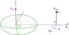 |
Fig. 1 Coordinate systems used to define the shape and position of each star. The companion is located on the positive x-axis and the angular momentum vector for the orbital motion is parallel to the z-axis. The inclination of the orbital axis to the line of sight is i. The origin of the (u,v,w) coordinate system is at the centre-of-mass of the binary system. Other symbols are defined in the text. |
2.2. Star shapes
The shape of the star is approximated by a triaxial ellipsoid centred at a position (x,y,z) = (D,0,0) with semi-axes (A,B,C) aligned with the x, y and z axes, respectively, i.e. 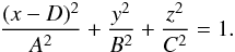 All lengths are relative to the semi-major axis of the binary orbit. This is the approximation that was also used in the WINK light curve model (Wood 1971). Three methods can be used to determine the values of A − D. The simplest model is a spherical star of radius R centred at the centre-of-mass, for which A = B = C = R and D = 0. This model can be very useful for rapidly calculating a large number of light curves and is accurate enough for many cases. The Roche potential is widely used to approximate stellar shapes in light curve models. I have used the definition of this potential described by Wilson (1979), which includes a modification of the potential to allow for non-synchronous rotation of the star. The direction of the star’s rotational angular momentum vector, Lrot is assumed to be parallel to Lorb. The values of A − D are set by requiring that the value of this potential is equal at the six points where the ellipsoid intersects the x, y and z axes, i.e. the ellipsoid matches the location of an equipotential surface at these points. The Roche potential makes the assumption that the entire mass of the star is located at the centre of mass. More realistically, the mass distribution within a star can be calculated by assuming a polytropic equation of state. The equilibrium shape of a polytrope in the tidal field of a companion star has been calculated by Chandrasekhar (1933b). Chandrasekhar also calculated the effect of rotation on a polytropic star (Chandrasekhar 1933a) and discussed how, to a good approximation, rotation and tidal distortion can be treated independently to describe the shape of a star in a binary system (Chandrasekhar 1933c). I take the same approach and use Chandrasekhar’s calculations for the tidal distortion of a polytrope. For the rotational distortion the model interpolates the results tabulated by James (1964) for polytropes with polytropic index n = 1.5 or n = 3. A polytrope with n = 1.5 is a good approximation for stars where energy transport in the outer layers is dominated by convection and for gaseous planets, n = 3 is more appropriate for stars whose structure is dominated by radiation pressure. The offset of the star towards the companion is D = Δ3q(R/d)4(R/a) where the coefficient Δ3 is taken from Table VI of Chandrasekhar (1933b), d is the distance between the stars’ centres-of-mass, and q is the mass ratio. The coefficients ξp and ξe from Table 1 of James (1964) are used to calculate the polar and equatorial radii of an oblate spheroid centred at (x,y,z) = (D,0,0) with its minor axis parallel to Lrot. I then apply the model for the tidal distortion of this surface given in Eq. (35) of Chandrasekhar (1933b) to this oblate spheroid, again assuming that Lrot is parallel to Lorb.
For eccentric orbits I model the star using the equilibrium shape at each point in the orbit, i.e. I do not include any dynamical tidal effects in the model. The shape of the star will vary through the orbit as a result of the variations in the tidal field due to the companion but the volume is assumed to be constant (Chandrasekhar 1933b).
2.3. Star positions
Times are measured relative to a reference time t0 when the separation of the stars’ centres-of-mass projected on the sky is at a minimum. The two stars in the binary are labelled 1 and 2 with star 1 furthest from the observer at time t0, i.e. star 1 will be eclipsed by star 2 at time t0 if the inclination of the binary is i = 90°. If star 1 is hotter than star 2 and the orbit is approximately circular then this eclipse will be the primary eclipse, i.e. deeper than the secondary eclipse that will occur approximately half an orbit later. I assume that the stars follow Keplerian orbits with fixed orbital eccentricity, e. At time t0 the longitude of periastron for star 1 is ω0 and the orbital inclination i0. Apsidal motion can be included by specifying a non-zero value for  , so that the longitude of periastron for star 1 at time ti is
  and the longitude of periastron for star 2 is ω2 = ω1 + π. Similarly, the inclination of the orbit at time ti is assumed to be
  . The longitude of periastron is not defined for circular orbits, in which case I fix ω0 = 0.
At time t0 the true anomaly of star 1 is ν1,0 ≈ π/ 2 − ω0. The exact value of ν1,0 is calculated by finding the value of ν1,0 that minimises the projected separation between the stars’ centres-of-mass (Lacy 1992). At other times the position of star 1 is calculated using Kepler’s equation, M = E − esinE, to find the eccentric anomaly E from the mean anomaly M = 2π(ti − t0) /Pa, where the anomalistic period Pa is assumed to be constant. The true anomaly of star 1 is then ![\begin{eqnarray*} \nu_{\rm 1} = 2\tan^{-1}\left[\sqrt{\frac{1+e}{1-e}}\tan(E/2)\right], \end{eqnarray*}](/articles/aa/full_html/2016/07/aa28579-16/aa28579-16-eq51.png) and ν2 = ν1 + π for star 2. The angle from the x-axis towards the projection of the line of sight in the x-y plane for star 1 is then φ = ν1 − π/ 2 + ω measured clock-wise looking towards the origin along the z-axis (Fig. 1), and similarly for star 2.
and ν2 = ν1 + π for star 2. The angle from the x-axis towards the projection of the line of sight in the x-y plane for star 1 is then φ = ν1 − π/ 2 + ω measured clock-wise looking towards the origin along the z-axis (Fig. 1), and similarly for star 2.
The separation of the centres-of-mass at time ti relative to the semi-major axis of the orbit is d = 1 − ecos(E) so the position of star 1 in the observer’s (u,v,w) coordinate system defined previously is (u1,v1,w1), where 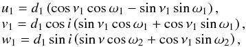 d1 = dq/ (1 + q), and q = M2/M1 is the mass ratio. The apparent position on the sky of star 1 at time ti accounting for the light travel time across the orbit is given to a very good approximation by the actual position of star 1 at time t1 = ti + w1a/c, where c is the speed of light and a is the semi-major axis of the binary orbit. The light travel time across the orbit can be ignored by setting a = 0, but in this case the Doppler boosting effects discussed below with not be calculated. The position of star 2 is calculated in a similar way using ν2 = ν1 + π and r2 = d/ (1 + q). If a> 0 then Eq. (25) from Borkovits et al. (2015) is used to calculate a correction to the value of t0 for the light travel time across the orbit so that the apparent time of mid-eclipse occurs at the time t0 specified by the user.
2.4. Specific intensity distribution
The specific intensity of the point (s,t) on the stellar disc is given by  where ℐ0 is a constant for each star, U(μ) is the limb darkening law, G(s,t) accounts for gravity darkening and the term H(s,t)UH(μ) accounts for the irradiation of the star by its companion.
I have implement several limb-darkening laws to account for the variation of specific intensity with the cosine of the viewing angle, μ. The simplest limb-darkening law is linear limb darkening, which depends only on a single limb darkening parameter, u (Schwarzschild 1906):  Two-parameter limb-darkening laws implemented in ellc include a square-root limb-darkening law (Diaz-Cordoves & Gimenez 1992)
  an exponential limb-darkening law (Claret & Hauschildt 2003)
  alogarithmic limb-darkening law (Klinglesmith & Sobieski 1970)
  and a quadratic limb-darkening law (Kopal 1950)
  Claret (2000) introduced the following four-parameter limb darkening law that has also been implemented:
 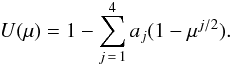 The 3-parameter limb-darkening law defined (Sing et al. 2009) which is equivalent to Claret four-parameter with c1 = 0 has also been implemented.
For gravity darkening I assume that the specific intensity can be related to the local gravity by a power law with exponent y(λ). Note that y(λ) is a wavelength dependent quantity, not the bolometric gravity darkening exponent often used in other light curve models. Appropriate values of y(λ) and limb-darkening coefficients for various passbands can be found in Claret & Bloemen (2011). The local gravity can be calculated using the gradient of the Roche potential at any given point on the surface, but this calculation has a significant impact of the speed of the program if it is done for every integration point used in the calculation. Instead, by default the program calculates the gradient of the Roche potential at the four points (x,y,z) = (D + A,0,0), (D − A,0,0), (D,B,0) and (D,0,C) and then uses a simple function to interpolate the value of the surface gravity at other points on the stellar surface. An option is provided to use the point-by-point calculation of the local surface gravity so that the impact of this approximation can be quantified. For example, in the case of KPD 1946+4340 shown below we used this option to check that using the default method changes the light curve by less than 250 ppm at all phases.
Irradiation of the star by its companion can be difficult to deal with because the incident energy of the companion changes the thermal structure of its atmosphere. As a result, the emergent spectrum can be very different to that of the incident radiation, e.g., ultraviolet photons from the companion can be absorbed and re-emitted as emission lines at optical wavelengths. The change in thermal structure also changes the local limb-darkening law (Vaz & Nordlund 1985). In extreme cases, the incident radiation may produce an optically thin layer in the upper layer of the star’s atmosphere that will then appear limb-brightened. If the incident radiation is absorbed and re-emitted with a different spectrum then a complete physical model would require as input an accurate estimate of the incident flux and its spectrum. This spectrum may be difficult to observe and hard to predict accurately from models, particularly at ultraviolet wavelengths where the majority of the flux from hot stars is emitted, interstellar absorption is severe and the models are strongly affected by line-blanketing effects. In principle, calculating the spectrum of the incident radiation at each point on the star’s surface would require integration of the emergent spectrum over the visible surface of the companion accounting for the variation in limb darkening and gravity darkening with wavelength, and then iterating to account for the radiation re-emitted by the star back to its companion. For exoplanets the situation becomes even more complicated because of the possibilty of advection, i.e. the incident energy may not be emitted at the location where it is absorbed. As a result, implementing a prescription for irradiation based on physical models in a general purpose light curve model would lead to a large computational overhead, the results may then depend on model parameters in a way that is difficult for the user to understand and control, and the results may be no more accurate than a more simplistic approach. For these reasons I have implemented a simple prescription for irradiation based on three parameters that relate directly to specific intensity distribution on the surface of the star and its angular dependence. In cases where an accurate physical model for irradiation is available, e.g., simple reflection by scattering from free electrons, it is then possible to set the values of these parameters appropriately. For cases of weak irradiation, the simplicity of the model will not be an issue because the effect on the resulting light curves will be small. If the observed light curves are clearly affected by irradiation then some or all of the parameters can be included as free parameters in the fit in order to explore how much the parameters of interest are affected by the way irradiation is dealt with, or to gain some insight into the physics of irradiation.
The specific intensity of the point (s,t) includes the term H(s,t)UH(μ) to deal with irradiation. The factor UH(μ) is a linear limb darkening law with coefficient uH. The angle between the local surface normal and the vector from the point (s,t) to the centre of the companion, γ, is calculated by assuming that the surface of the ellipsoid can be approximated by a sphere with the same radius as the distance of the point from the centre of the ellipsoid, r(s,t). The distance from the point (s,t) to the centre of the companion is d and the companion is assumed to be a sphere of radius  . If cosγ> Δ = (r(s,t) − rc) /d then the entire disc of the companion is visible so I take the irradiating flux to be
 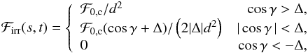 where ℱ0,c is the specific intensity integrated over the visible hemisphere of the companion for a distant observer viewing the companion along the x axis. This integration is done using Eq. (1) discussed below. The specific intensity normal to the surface is taken to be
 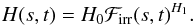 Several geometrical factors of order 1, albedo effects and the redistribution of incident energy into the observed wavelength region are all subsumed into the parameter H0. The parameter H1 can be used to give some control over how the specific intensity depends on the strength of the irradiation. Using H1 ≫ 1 will create a “hot spot” near the point closest to the companion, whereas H1 = 0 will result in approximately uniform brightness for all points with cosγ> Δ.
2.5. Integration
To obtain the observed flux the specific intensity must be integrated over the visible area of the star. This integration is implemented using a combination of numerical Gaussian-Legendre quadrature and exact analytical expressions for the areas of overlapping ellipses. The integral required can be written 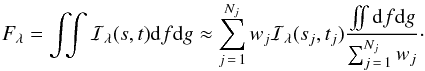 (1)The first summation in this expression represents Gaussian-Legendre quadrature over a two-dimensional non-rectangular grid of Nj points at locations (sj,tj) with weights wj. The size of the grid is specified by the number of grid points along the major axis on the ellipse. In the current implementation this value is either 4, 8, 16, 24 or 32. The distribution of the integration points is approximately uniform over the visible area. The summation in the denominator of the ratio is an estimate of the area of the visible stellar disc calculated in the same way. The actual area of the stellar disc that is visible is given by the integral in the numerator of the ratio, and can be calculated exactly since it is either the area of an ellipse, or the difference between this area and the area common to two overlapping ellipses. The ratio of the integral and sum has a fixed value for a given combination of Nj, (sj,tj) and wj, and serves as a correction that improves the accuracy of the numerical integration. An alternative view of the same expression is that flux is calculated from the visible area of the ellipse, which can be calculated exactly, weighted by the average intensity over the visible area, which is calculated by numerical integration. The calculation of the overlap area of two ellipses requires a very robust algorithm to calculate the number and positions of the intersections between two ellipses. The algorithm I have developed is described in Appendix A.
2.6. Flux scale and surface brightness ratio
The surface brightness ratio is an ambiguous quantity for limb-darkened stars in a binary that do not emit isotropically. To define a flux scale in ellc I first set the specific intensity normal to the surface at the point on star 1 closest to its companion to 1, i.e. ℐ0,1 = 1. I then use Eq. (1) to calculate ℱ0,1, the integral of the surface-brightness distribution for the star 1 for a distant observer viewing the star along the x-axis. This calculation step ignores eclipses, spots and heating effects by the companion, but does include the tidal distortion terms. The same calculation for star 2 with ℐ0,2 = 1 gives the quantity ℱ0,2(ℐ0,2 = 1) which is then used to set the value of ℐ0,2 used in all subsequent steps in the calculation such that  where Sλ is the value specified by the user for the disc-averaged surface brightness ratio at the wavelength of observation λ.
The next step in the calculation is to set a normalising factor for the output light curves. This is done in the same way as the calculation for ℱ0,1 but in this case the irradiation factor is included. This calculation yields two normalising factor ℱN,1 and ℱN,2. The calculation of the light curve then proceeds using Eq. (1) to calculate the ℱi,1 and ℱi,2, the apparent fluxes at times ti for stars 1 and 2, respectively, including irradiation, eclipses, star spots and Doppler boosting. The values of ℱi,1 and ℱi,2 can be obtained directly using the routine fluxes in the python module ellc. The light curve generated by the routine lc in the same module returns the value 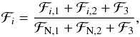 where ℱ3 = ℓ3(ℱN,1 + ℱN,2) and ℓ3 is a value for “third-light” specified by the user.
2.7. Simplified reflection effect
Integrating the illumination pattern on one star by the other can result in severe numerical noise in the light curve due to the sharp boundary between the illuminated and non-illuminated hemispheres if a sparse integration grid, must be used, e.g., if a large number of approximate light curves need to be calculated to explore the parameter space of a least-squares fitting problem. To avoid this problem a simplified model for the reflection effect is available which is useful in cases where the amplitude of the reflection effect is low. In this simplified model the flux of each star increased by an amount ![\begin{eqnarray*} {\cal R}_{1,2} = \alpha_{1,2}{\cal I}_{0,(2,1)}(R_{1,2}/d)^2\left[ \frac{1}{2} + \frac{1}{2}\sin^2i\sin^2\phi_{1,2} \pm \sin i\sin\phi_{1,2}\right], \end{eqnarray*}](/articles/aa/full_html/2016/07/aa28579-16/aa28579-16-eq117.png) where the positive and negative cases of the final term apply to stars 1 and 2, respectively. During the eclipse this quantity is reduced by a factor equal to the fractional loss of flux from the eclipse star. This is the same model for the reflection effect used in ebop (Etzel 1981) except that ebop includes a factor (R1,2/a)2 in “geometric reflection coefficient” whereas I use the factor (R1,2/d)2 explicitly in the model.
where the positive and negative cases of the final term apply to stars 1 and 2, respectively. During the eclipse this quantity is reduced by a factor equal to the fractional loss of flux from the eclipse star. This is the same model for the reflection effect used in ebop (Etzel 1981) except that ebop includes a factor (R1,2/a)2 in “geometric reflection coefficient” whereas I use the factor (R1,2/d)2 explicitly in the model.
2.8. Radial velocity
If the semi-major axis of the binary orbit (a) is set to a non-zero value then the radial velocity (vr) of each star is calculated. The centre-of-mass radial velocity is calculated from the Keplerian orbit of the star and can be obtained using the routine rv in the ellc python module. A check is made in the program for a non-zero value of a and an orbital period value Pa = 1, which is assumed to be an error in input because Pa = 1 is used to denote that the input times for calculation are in phase units, not days as required for the correct calculation of the radial velocity.
The default behaviour in the current version of rv is to return radial velocity values that are weighted by the flux from every point on the visible surface of the star (“flux-weighted radial velocity”). These are calculated in the same way as the flux values used for the calculation of the light curves. The projected rotational velocity at every point on the star’s surface can be calculated using the asynchronous rotation factor, Frot = Pa/Prot, that is also used to define the shape of the star with rotation period Prot. Alternatively, the projected equatorial rotation velocity at the stars’ equator, Vrotsini, can be used to determine the projected rotational velocity over the stellar surface. The effect of star spots on the flux-weighted radial velocities is accounted for by multiplying the flux-deficit due to the spot by the projected rotational velocity at its centre. This approximation will not be accurate for large spots.
The effect of eclipses on the flux-weighted radial velocity is accounted for and so ellc can be used to model the Rossiter-McLaughlin (R-M) effect for stars in which the rotation axis is aligned with the orbital axis. It is also possible with ellc to model the R-M effect for a spherical star eclipsed by star or planet described by the Roche potential, a polytrope or a sphere for which the projection of the rotation axis on the sky during the eclipse is at an angle λ to the orbital axis, as defined by Ohta et al. (2005).
2.9. Doppler boosting
The flux-weighted radial velocity can be used to correct the apparent flux for the effects of Doppler boosting, which increases the flux by a factor (1 − vr/c)3, and the Doppler shift, which reduces the flux by a factor ≈(1 − vr/c)2 that depends on the wavelength gradient of the stellar spectrum (Maxted et al. 2000). For radial velocities vr ≪ c the two effects can be combined into a single factor  , where
  is calculated separately (Bloemen et al. 2011), or can be set to zero to ignore these effects. The flux-weighted radial velocity accounts for the eclipse of the star and so ellc can be used to model the photometric R-M effect (see Sect. 3.5, below). Using centre-of-mass radial velocities with Doppler boosting gives inconsistent results for the eclipses in the light curves (because the photometric R-M effect is not included) and so is not recommended.
2.10. Star spots
The effect of circular spots on the light curve of a spherical star with quadratic limb-darkening have been calculated by Eker (1994a) and the resulting integrals are provided in convenient form in the appendix to that paper together with an erratum (Eker 1994b). I use these equations in ellc to calculate the variation in flux from each star due to spots in the model. In cases where the limb-darkening law used is not quadratic I set the limb-darkening coefficients used in the spot model so that it matches the actual limb-darkening law used at the points μ = 0,0.5 and 1. In cases where the spot is eclipsed by the companion I reduce the effect of the spot by a factor equal to the fraction of the spot covered by the companion. The position of the centre of the spot on the sky is calculated based on its longitude and latitude on the triaxial ellipsoid and its shape is calculated by approximating the surface of the triaxial ellipsoid by a sphere with the same radius as the distance from the centre of the spot to the centre of the ellipsoid. The calculation of the eclipsed area is straightforward if it is not on the limb of the star because the projected shapes of the spot and the companion are both ellipses. The calculation is more difficult if the spot intersects the limb of the star because it involves the intersection of two ellipses and a circle. The area required can be found as the sum of various ellipse segments and triangles so is quick to calculate, but this does require some effort to implement as there are approximately 90 different possible configurations for the two ellipses and the circle that must be considered.
3. Examples
In this section I test the reliability of ellc by comparing it to other binary star models and show how ellc can be used to analyse light curves and radial velocity observations for eclipsing binary star systems using Monte Carlo methods.
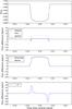 |
Fig. 2 Upper panel: light curve for a planet on an eccentric orbit with i = 90° calculated using batman. Upper-middle panel: difference between the light curves calculated using ellc for a spherical planet with the grid sizes indicated and with batman for the case i = 90°. Lower-middle panel: difference between the light curves calculated using ellc with the default grid size for planet described by either a Roche potential or a polytrope with index n = 1.5 and with batman for the case i = 90°. Lower panel: difference between the light curves calculated using ellc with the default grid size and a spherical planet and with batman for an eccentric orbit with i = 87°. The difference in flux of approximately 50 ppm during ingress and egress is the result of an inaccurate estimate for the time of periastron in the batman model. |
3.1. batman
Kreidberg (2015) has developed a python package for modelling exoplanet transit and eclipse light curves with an algorithm that provides very high numerical precision. I have used batman to evaluate the numerical precision of the light curves calculated using ellc. The upper panel of Fig. 2 shows the light curve calculated using batman version 2.1.0 for the case of the transit of a spherical star by a spherical planet with a radius of 0.1 stellar radii (Rp = 0.1 R⋆). The semi-major axis of the orbit is 10 R⋆ and the inclination of the orbit is i = 90°. The quadratic limb-darkening coefficients are c1 = 0.1 and c2 = 0.3. The eccentricity of the orbit is e = 0.1 and the longitude of periastron is ω = 60°. The next panel down in this figure shows the difference between this light curve and light curves calculated using ellc with a grid size of 8 (“sparse”), 16 (“default”) or 24 (“fine”). The models agree to better than 10ppm at all phases of the transit for the sparse grid and to within a few ppm for the default and fine grids. This level of precision is more than sufficient given the level of systematic error due to astrophysical phenomena not included in these models. To give just one example, the next panel down in Fig. 2 shows the difference between the same light curve calculated with batman and light curves calculated using ellc using either a Roche potential or a polytrope with n = 1.5 to calculate the shape of the planet assuming that the mass ratio is q = 0.001. The difference of about 15 ppm seen in this panel is a due to the systematic error in light curve calculated with batman that arises from using a sphere to approximate the shape of a tidally disorted planet. The current version of batman does not include the option of calculating light curves for non-spherical planets. This systematic error can result in the measured radius being to low by 1−10% for a typical hot Jupiter systems (Leconte et al. 2011a,b).
I also tested ellc against the results from batman for the same planetary system viewed at an inclination i = 87°. The results shown in the lower panel of Fig. 2 show differences of about 50 ppm between the two light curves during ingress and egress. Inspection of the source code for batman shows that the time of periastron relative to the time of mid-transit is calculated using an expression that assumes i = 90°. This approximation is not justified at this level of precision for inclinations i ≠ 90°. This problem was fixed in batman version 2.0.0.
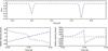 |
Fig. 3 Comparison of the light curves and radial velocity curves for a binary system showing double-partial eclipses computed using Nightfall (dashed lines) and ellc (dotted lines). |
3.2. Double-partial eclipses
If two stars in an orbit with i ≈ 90 are of similar size and one of the stars rotates close to its break-up velocity, then the rapidly rotating star will be significantly oblate. This makes it possible for the eclipse of this oblate star to produce a configuration I call a “double-partial eclipse” in which the poles of the oblate star are eclipsed while the equator is visible on both sides of the slowly-rotating star. The effect on the light curve of this configuration is quite subtle, but the Rossiter-McLaghlin (R-M) effect during the double-partial eclipse has a characteristic large and rapid change from positive to negative velocity at the mid-point of the eclipse. To test whether ellc can reproduce this effect correctly I compared light curves and radial velocity curves for a hypothetical binary system with double-partial eclipses calculated with ellc to those calculated using Nightfall1 (Wichmann 2011). The results are shown in Fig. 3. The details of these simulations can be found in the information provided with the software package, which includes the python scripts used to generate this plot and the configuration file for Nightfall. There are small differences between the light curves and radial velocity curves generated by the two models, but overall the agreement betweed the two models is very good. The rapid change from positive to negative velocity at the mid-point of the eclipse is seen very clearly in the radial velocity curve generated by ellc.
The calculation of light curves in 11 bands and radial velocites at 8192 phase points using Nightfall version 1.88 takes 2.3 s on a MacBook Pro with a 2 GHz Intel Core i7 CPU. The time taken to calculate a light curve in a single band and 2 radial velocity curves with ellc and to generate the plot on the same machine is 2.5 s. I also attempted to use Nightfall to generate a similar plot for an eccentric orbit but found that there is a bug in this version of the program that inverts the shape of the R-M effect for eccentric orbits. The execution time in this case was 113.4 s. This is much slower than the calculation for the circular orbit because Nightfall uses a grid of points in 3-dimensional space to represent the stars. There is a large overhead required to re-calculate the positions of all the points on this grid at each phase point to account for the varying potential in an eccentric orbit. There is no significant increase in the execution time for ellc for an eccentric orbit compared to a circular orbit in this case.
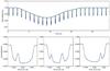 |
Fig. 4 Comparison of the light curves for a spherical star with two circular spots eclipsed by a spherical dark body calculated using ellc (thin line) and KSint (points). |
3.3. KSint
KSint is a fast numerical algorithm for accurately calculating light curves for transiting extrasolar planets orbiting spotted stars (Pál 2012; Montalto et al. 2014). The model assumes that the star and planet are spherical. As with ellc, the spot profile is defined from the interception of a cone with its vertex at the centre of the sphere with the surface of the sphere. I have used ellc and KSint version 1.0 to calculate the light curve for a spherical star with a rotation period of 23.9 days with two dark spots and a planetary companion on a circular orbit with a period of 1 day and an inclination i = 90°. The radius of the planet is 0.1 stellar radii (Rp = 0.1 R⋆) and the semi-major axis of the orbit is 2.765 R⋆. In reality a planet on such a short-period orbit would be appreciably non-spherical, but I have assumed that the planet is spherical for the calculation of the light curve with ellc so that the results are directly comparable to those calculated with KSint. The limb darkening coefficients for the quadratic limb darkening law are c1 = 0.4 and c2 = 0.3. The angular radius of one spot (≈5.74°) is set such that its projected size on the sky is the same as the planet. This gives a good test of the numerical stability of the algorithm used to calculate the intersections between the projected edges of the spot and planet. The radius of the other spot is a factor  larger. The dimming factor for both spots is 0.5. Both stars are on the stellar equator and are separated by an angle of 60°. The results are shown in Fig. 4. A few of the points in the light curve calculated using KSint are badly affected by numerical noise, e.g., the low points in the ranges 19.88−19.95 days and 23.86−23.94 days, and a few high points near the first and last contact points of some transits. By contrast, the light curve calculated using ellc shows very little numerical noise. In other regions of the light curve, the agreement between the two models is excellent.
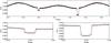 |
Fig. 5 Phase-binned Kepler short-cadence data for KPD 1946+4340 (points) compared to light curves generated using ellc using the Roche potential (solid line) and a polytrope with index n = 1.5 (dashed line). |
3.4. KPD 1946+4340
KPD 1946+4340 is a subdwarf-B star in a short-period binary system (P ≈ 0.4 d) with a white dwarf companion (Bloemen et al. 2011). This configuration together with the very high quality light curve of this binary obtained by the Kepler mission make KPD 1946+4340 a useful test case for the calculation of the ellipsoidal effect and Doppler boosting with ellc. I downloaded all the observations of KPD 1946+4340 obtained with Kepler in short-cadence mode from the Kepler data archive2 and used the flux values provided in the column pdcsap_flux of the archive data tables to create the phase-binned light curve shown in Fig. 5. This phase-binned light curve is formed from 1 007 160 photometric measurements from Kepler excluding flagged data points and a few obvious outliers. The ephemeris used to calculate the phase is from Bloemen et al. (2011) converted to the Barycentric Kepler Julian date (BKJD) time system used for the Kepler archive data, i.e.  The eclipse of the white dwarf occurs at phase 0. The ellipsoidal variation due to the tidal distortion of the sdB star by the much-fainter white dwarf companion can be seen as a smooth variation with a period half that of the orbital period. The Doppler boosting of the light from the sdB star is also obvious from the asymmetry in the light curve between phase 0.25 when its is receeding from the observer and phase 0.75 when it is approaching. These effects are only obvious because of the superb quality of this light curve – the rms scatter is approximately 0.01% and the entire flux range plotted in Fig. 5 is less than 1%.
I used the parameters for this binary system from Bloemen et al. (2011) to simulate the light curve of KPD 1946+4340 assuming either a Roche potential for the stars or a polytrope with index n = 1.5. Other details of the simulation can be found by inspection of the python script used to generate this figure that is included with the software distribution. The simulated light curve using the Roche potential gives an excellent match to the light curve at all phases. In particular, the asymmetry in the light curve due to Doppler boosting is very well reproduced when the orbital velocity of the sdB star (which dominates the flux) is set to the value measured from its orbital Doppler shift. Using a polytrope to describe the shape of the sdB star results in a worse match to the ellipsoidal variation, but the parameters used for this simulation were based on a least-squares fit to the Kepler light curve of KPD 1946+4340 using a Roche potenttial, so it may be that a better fit to the light curve can be achieved for a polytropic model by adjusting the other parameters in the model. This would certainly be an interesting exercise now that there is more than 20 times as much Kepler data available for this star than was available at the time of the study by Bloemen et al. A full analysis will require very careful handling of any systematic errors in the data since the signal being analysed here are very small. This analysis is beyond the scope of this description of the software, but I demonstrate below that ellc can be used to analyse high-quality data such as these using Monte Carlo techniques.
3.5. Photometric R-M effect
The photometric R-M effect is essentially the same phenomenon as the spectroscopic R-M effect measured using the Doppler shift of stellar spectral lines. The variations in apparent flux are the result of Doppler boosting of the light from different parts of a rotating star during an eclipse (Hills & Dale 1974). The amplitude of the signal is generally very small so there are no reported detections of this phenomenon to-date. Groot (2012) has discussed the prospects for detecting this signal using simulations that include limb darkening and obliquity but that neglect the oblateness of the stars. Figure 6 shows a simulation using ellc for a pair of white dwarfs in a binary system with parameters similar to those used by Groot, i.e. an orbital period of 39.1 min, i = 90° and rotational velocities close to their maximum possible values. The details of this simulation can be found by inspection of the python script used to generate this figure that is included with the software distribution. To estimate the maximum possible size of the photometric R-M effect Groot compared the light curves for the stars rotating at their break-up velocity to stars rotating synchronously with the orbit. A similar comparison with ellc shows that the differences in the light curves are completely dominated by the change in shape of the stars and the change in the surface brightness distribution due to gravity darkening. Instead, to generate the flux difference due to the photometric R-M effect shown in Fig. 6 I calculated the light curves for stars rotating near their break-up velocity with both prograde and retrograde rotation and have plotted half of the difference between these results. The shape and amplitude of the signal are similar to the results shown by Groot. Also shown in Fig. 6 is the photometric R-M effect for the same system assuming that the sky-projected rotation axis is misaligned with the rotation axis by an angle λ = 60°. This light curve was calculated for spherical stars because the current version of ellc does not include misaligned rotation for non-spherical stars.
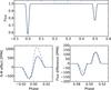 |
Fig. 6 Simulation of the photometric Rossiter-McLaughlin (R-M) effect for a pair of white dwarf stars rotating close to their break-up velocity in an eclipsing binary with a period of 39.1 min. Upper panels: light curve of the binary; the two lower panels: contribution to this light curve due to the photometric R-M effect. In all panels, the solid line is calculated using Roche geometry for stars with rotation axes aligned with the orbital axis and dashed lines are for models of spherical stars with λ = 60°. |
3.6. GD448
GD448 is a non-eclipsing, short-period (P = 0.103 d) M-dwarf – white-dwarf binary system (Maxted et al. 1998). This binary system shows a reflection effect in the light curve with an amplitude of about 0.1 mag in the I-band. Fig. 7 shows the I-band light curve of GD448 simulated using Nightfall using the parameters for the binary from Maxted et al. (1998). The effective temperatures of the stars used in this simulation were 19 000 K and 3000 K, respectively. Further details of the simulation can be found by inspection of the python script used to generate this figure and other files that are included with the software distribution. The amplitude of the reflection effect is underestimated in this simulation, partly because the model atmospheres available in Nightfall are not accurate when applied to a white dwarf. It would be possible to get a better match the observed amplitude of the reflection effect in GD448 by adjusting the assumed albedo value in the model from its default value of 0.5. Also shown in Fig. 7 are light curves simulated using ellc with two sets of irradiation parameters H0,H1 = (0.6,3.5) and (1.0,1.5). These values were set “by-eye” to produce a similar shape and amplitude to the reflection effect calculated using Nightfall.This demonstrates that ellc can be used to calculate light curves that include the reflection effect using reasonable values for the parameters in the irradiation model but, as with other light curve models, these free parameters need to be adjusted to match the shape and amplitude of the reflection effect in the observed light curves of actual binary stars. The result of using the simplified reflection effect model is also shown in Fig. 7 with the reflection coefficient adjusting “by-eye” to match the amplitude of the reflection effect calculated using Nightfall.
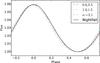 |
Fig. 7 Light curves of the short-period M-dwarf – white-dwarf binary GD448 simulated using Nightfall and using ellc with two sets of heating/irradiation parameters H0,H1, as indicated, and also using a simplified model of the reflection effect with α = 2.1. |
3.7. 1SWASP J011351.29+314909.7
1SWASP J011351.29+314909.7 (J0113+31) is a metal-poor ([Fe/H] = − 0.40 ± 0.04), solar-type star eclipsed by a low-mass M-type dwarf in a binary with an orbital period P ≈ 14.3 days and an eccentric orbit (e ≈ 0.3). This eclipsing binary was discovered using photometry from the WASP project because it shows a transit in the light curve with a depth of about 2.5%. Gómez Maqueo Chew et al. (2014, hereafter GMC+2014) have presented a thorough analysis of this binary system based on additional photometry at optical wavelengths through the primary eclipse (transit) from three instruments (NITES, OED, and BYU) and J-band photometry of the secondary eclipse obtained with the FLAMINGOS instrument and Kitt Peak National Observatory (KPNO). Full details of these observations are given in GMC+2014.
I have used ellc to analyse these observations of J0113+31. To explore the model parameter space I used emcee (Foreman-Mackey et al. 2013), a python implementation of an affine invariant Markov chain Monte Carlo (MCMC) ensemble sampler. The free parameters in the fit were r1 and r2 – the radii of the stars relative to the semi-major axis of the binary, i – the inclination,  and
and  , SJ – the surface brightess ratio in the J-band, and K1 – the semi-amplitude of the primary star’s spectroscopic orbit. The eccentricity and orientation of the orbit are described by the parameters fs and fc because these have a uniform prior probability distribution. Uniform priors were also adopted for the other parmeters in the analysis. There are 7 free parameters and I used 50 walkers with 1000 chain steps to calculate their posterior probability distribution. To speed-up the calculation I only included WASP data within 0.02 phase units of the transit in the analysis. The NITES light curve was observed at high cadence so I used ellc to calculate this light curve for 1-in-10 of the observed data points and then used an option implemented in ellc to interpolate the light curve to other times of observation. The walkers were initialised using randomly selected parameter values from Gaussian distributions with mean and standard deviation set from the results of some test runs of emcee. The convergence of the chain was judged “by-eye” by inspection of the parameter values and the log likelihood as a function of step number. The best-fit values and standard errors of selected model parameters and derived values given in Table 1 were calculated from the median and standard deviation of parameter values in the chain excluding the first 500 steps of each walker. The joint posterior probability distributions for the parameters are shown in Fig. 9. Further details of the analysis can be found by inspection of the python script used to generate these figure that is included with the software distribution.
The total number of chain steps is 350 000 and the acceptance fraction for each walker is ≈0.5 so the number of simulated data sets calculated to produce these results is ≈700 000. The calculation took 17 min using 4 threads on a MacBook Pro with a 2 GHz Intel Core i7 CPU. For comparison, GMC+2014 used a Linux cluster with over 6000 processor cores and a peak performance of roughly 24.5 TFLOPS to sample 36 972 combinations of four parameters (i, effective temperature ratio T1/T2, r1 and r2) using the Wilson-Devinney binary star model within the PHOEBE software package (Prša & Zwitter 2005; Wilson 1979). They did not include the WASP and NITES photometry in their analysis. The computation of 10 000 light curves with this cluster took about 6 h (Hebb, priv. comm.)
The agreement between my results and those of GMC+2014 is excellent and the precision of radius measurements has been much improved. The small change in the value of K1 may be the result of an offset between radial velocity measurements obtained with two different instruments that has not be included in my analysis. It is beyond the scope of this paper to interpret these results (which are consistent with those from GMC+2014) and further analysis is required to determine the sensitivity of these results to important details such as the adopted limb-darkening coefficients. Nevertheless, it is clear that ellc makes it feasible to employ Monte Carlo methods to analyse light curves and radial velocity data for eclipsing binary stars and that it runs much faster than other binary star models when applied to binary stars with eccentric orbits.
Parameters for the eclipsing binary system J0113+31 using ellc and emcee.
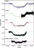 |
Fig. 8 Observed light curves for the eclipsing binary J0113+31 (points, Gómez Maqueo Chew et al. 2014) compared to light curves generated using ellc for the parameters shown in Table 1 (solid lines). |
3.8. HD 23642
The ellc package includes a python script called ellc_emcee.py that can be used to analyse a single light curve using the ellc binary star model. The best-fit light curve and the posterior probability distribution of the free parameters in the model are calculated using the emcee algorithm. The script prompts the user for the values of the fixed and free parameters and any priors to be imposed on the parameters of the problem. Output file names and other options such as the grid size can be set using command-line options. A log file is produced that includes a copy of the user input that can modified and then used directly as input into subsequent runs of ellc_emcee.py, e.g., for reanalysis of the same light curve with a different set of free parameters or different starting values for free parameters. Up to 2 spots per star can be included in the model. Limb-darkening and gravity-darkening are specified using the effective temperature and surface gravity of each star and the metallicity of the binary system. These parameters are then used to look-up the limb-darkening coefficients for a 4-parameter limb darkening law and the gravity-darkening coefficients for each star using linear interpolation in the tabulation of Claret & Bloemen (2011). Options to exclude data from the fit, interpolate the model across data, or to use numerical interpolation to account for the exposure time are all set using an integer flag value in the input light curve data.
To demonstrate some of the capabilities of ellc_emcee.py I have used this script to analyse the Kepler K2 light curve of HD 23642. This is an eclipsing binary in the Pleiades star cluster with an orbital period of about 2.5 days showing partial eclipses between two A-type stars (Southworth et al. 2005; David et al. 2016). I used the Kepler K2 data corrected for systematic errors using the algorithm of Vanderburg & Johnson (2014) for this analysis3. To speed-up the calculation I used interpolation to calculate the model values for approximately 3/4 of the observations between the eclipses and used the “very_sparse” grid size (Nj = 4) for the numerical integration of the fluxes from both stars. For observations through the eclipses numerical integration using 5 integration points was used to account for the integration time of 1766 s. The residuals from a preliminary fit to the data show that the scatter around the best fit is quite variable with time – there is a block of very good data with slightly noisier data either side – so I set the estimated standard error of each observation to one of three values according to the time of observation. The values were choosen to achieve a reduced χ2 value for the best fit model close to 1. I excluded 10 discrepant observations from the analysis. The MCMC chain was calculated using 40 walkers and 5000 steps. This calculation took 55 min using 8 threads on a MacBook Pro with a 2 GHz Intel Core i7 CPU.
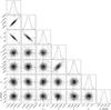 |
Fig. 9 Parameter correlation plots for my fit using ellc to the radial velocity data and light curves of the eclipsing binary J0113+31 from Gómez Maqueo Chew et al. (2014, GMC+2014). The adopted parameter values from GMC+2014 are indicated by lines/points in each panel. The contours in each panel show the 0.5-, 1-, 1.5- and 2-sigma confidence regions for each joint parameter distributions. Points outside the 2-sigma confidence region are individual steps from the emcee MCMC chain. |
The best-fit parameters and their standard errors are shown in Table 2. These were calculated using the median and standard deviation of approximately 145 000 values in the MCMC chain after discarding the first Nburn − in points from each walker, where Nburn − in is 4 × the largest autocorrelation length scale of the chains for all the parameters for each walker. The best-fit light curve model is shown in Fig. 10 and the distributions of selected parameters are shown in Fig. 11. Further details of the analysis can be found by inspection of the files included in the sub-directory examples/ellc_emcee that is included with the software distribution.
The agreement between my results and the analysis by David et al. (2016) using jktebop (Southworth 2013) is very good. There is a slight difference between the surface brightness ratio derived here and by David et al. (2016), partly because ellc defines this ratio for the stars when viewed at conjunction, whereas the ebop model used by David et al. defines this quantity at quadrature.
Parameters for the eclipsing binary system HD 23642 using ellc_emcee.
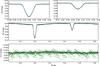 |
Fig. 10 Observed light curves for the eclipsing binary HD 23642 (points) compared to light curves generated using ellc_emcee.py for the parameters shown in Table 2 (solid lines). |
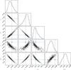 |
Fig. 11 Parameter correlation plots for selected parameters from my fit using ellc_emcee to the Kepler K2 light curve of HD 23642. The parameter values from the analysis of David et al. (2016) are indicated by lines/points in each panel. The contours in each panel show the 0.5-, 1-, 1.5- and 2-sigma confidence regions for each joint parameter distributions. Points outside the 2-sigma confidence region are individual steps from the emcee MCMC chain. |
4. Caveats
4.1. Radius and volume
The values of A − C that are used to specify the shape and size of the triaxial ellipsoid used in the calculation of the light curves are set by requiring that the volume of the ellipsoid is equal to the volume of a sphere with a radius R specified by the user, i.e. ABC = R3. For highly-distorted configurations this means that the volume of the star will not be the same as the volume of the triaxial ellipsoid used to approximate its shape. The correct way to deal with this difference will depend on the context in which ellc is being used. For example, if ellc is being used to perform a least-squares fit to a total eclipse of a star by a highly-distorted companion, it may be useful to calculate a correction based on the ratio of the projected area of a triaxial ellipsoid and an equipotential in the Roche potential viewed at mid-eclipse. Comparing the results obtained using ellc for spherical stars to those obtained for a Roche potential or a polytrope (as was done in Fig. 2) will give an upper limit to the size of any correction of this sort and so enable the user to determine if any correction is necessary.
4.2. Radial velocities
The flux-weighted radial velocity calculated using ellc may not accurately reproduce high-precision radial velocity measurements because some effects are not included and the definition of the Doppler shift is ambiguous if the line profiles that are measured are not symmetric. Effects missing from ellc include the tranverse Doppler effect and gravitational redshift. Asymmetric line profiles can be caused by convective blue-shift in cool stars, the R-M effect, pulsations, star spots, and instrumental effects. If the line profile is asymmetric then different methods to determine the Doppler shift will give different results, e.g., a best-fit Gaussian profile will give a different result to a value based on the maximum of a cross-correlation function. The size of these systematic errors will be comparable to the line-width and can only be properly accounted for by modelling both the observed line profile and the method used to measure the radial velocity.
4.3. Star spots
The light curves for stars with spots are calculated for a fixed value of the inclination (i0) and are then corrected for the effects of the eclipses. This means that light curves for spotted stars in binary systems with varying inclination will not be reliable. There are several approximations used to enable the efficient calculation of light curves and radial velocities for stars with spots in ellc. Detailed modelling of spotted stars is a problem well beyond the scope of what can be done with ellc or any other binary model that uses “dark circles” to approximate the complex phenomena associated with magnetic activity on cool stars. Nevertheless, the star spot model in ellc can be used to quantify approximately the likely effects of star spots on the light curves of cool stars if the user is aware of the limitations of the model.
4.4. Irradiation
No account is made for the irradiation of a star due to the its own radiation being re-emitted by its companion. Extreme values of the parameter H1 that determines the pattern of emission due to irradiation produce numerical noise in the light curves because numerical integration schemes do not produce accurate results if the integrand varies rapidly on a scale smaller than the grid point separation.
4.5. Bugs
The examples above show that ellc can be used to calculate accurate light curves and radial velocity curves for a wide range of binary systems. The tests described here have also highlighted some problems with the current versions of some existing binary star models. Similarly, there will certainly be combinations of input parameters for which ellc will not produce reliable results. Users of ellc are strongly advised to test the results produced by ellc against other binary star models to check that they are reliable. The ellc binary star model will be made available as an open-source software project so that users can contribute to its development, submit bug reports and access the latest version of the software4.
Acknowledgments
The coefficients of the quartic equation for the intersections of two ellipses are taken from a document “The Area of Intersecting Ellipses” by David Eberly that was published on the web site www.geometrictools.com, November 20, 2010. I am grateful to the authors of the software packages emcee, Nightfall and batman for their generosity in making their software available. The author gratefully acknowledges everybody who has contributed to make the Kepler Mission possible. Funding for the Kepler Mission is provided by NASA’s Science Mission Directorate. I thank the referee for their comments on the manuscript that have helped to clarify a few points in the text and that also led to a useful update to the software. This work was supported by the Science and Technology Facilities Council [ST/M001040/1].
References
- Auvergne, M., Bodin, P., Boisnard, L., et al. 2009, A&A, 506, 411 [NASA ADS] [CrossRef] [EDP Sciences] [Google Scholar]
- Bakos, G., Noyes, R. W., Kovács, G., et al. 2004, PASP, 116, 266 [NASA ADS] [CrossRef] [Google Scholar]
- Bloemen, S., Marsh, T. R., Østensen, R. H., et al. 2011, MNRAS, 410, 1787 [NASA ADS] [Google Scholar]
- Borkovits, T., Rappaport, S., Hajdu, T., & Sztakovics, J. 2015, MNRAS, 448, 946 [NASA ADS] [CrossRef] [Google Scholar]
- Bours, M. C. P., Marsh, T. R., Parsons, S. G., et al. 2014, MNRAS, 438, 3399 [NASA ADS] [CrossRef] [Google Scholar]
- Brogaard, K., VandenBerg, D. A., Bruntt, H., et al. 2012, A&A, 543, A106 [NASA ADS] [CrossRef] [EDP Sciences] [Google Scholar]
- Cardano, G. 1545, Ars Magna (Nurmberg) [Google Scholar]
- Chandrasekhar, S. 1933a, MNRAS, 93, 390 [NASA ADS] [CrossRef] [Google Scholar]
- Chandrasekhar, S. 1933b, MNRAS, 93, 449 [NASA ADS] [CrossRef] [Google Scholar]
- Chandrasekhar, S. 1933c, MNRAS, 93, 462 [NASA ADS] [Google Scholar]
- Claret, A. 2000, A&A, 363, 1081 [NASA ADS] [Google Scholar]
- Claret, A., & Bloemen, S. 2011, A&A, 529, A75 [NASA ADS] [CrossRef] [EDP Sciences] [Google Scholar]
- Claret, A., & Hauschildt, P. H. 2003, A&A, 412, 241 [NASA ADS] [CrossRef] [EDP Sciences] [Google Scholar]
- CollierCameron, A., Pollacco, D., Street, R. A., et al. 2006, MNRAS, 373, 799 [NASA ADS] [CrossRef] [Google Scholar]
- David, T. J., Conroy, K. E., Hillenbrand, L. A., et al. 2016, AJ, 151, 112 [NASA ADS] [CrossRef] [Google Scholar]
- Delrez, L., Santerne, A., Almenara, J.-M., et al. 2015, MNRAS, submitted [arXiv:1506.02471] [Google Scholar]
- Diaz-Cordoves, J., & Gimenez, A. 1992, A&A, 259, 227 [NASA ADS] [Google Scholar]
- Dischler, J., & Söderhjelm, S. 2005, in The Three-Dimensional Universe with Gaia, eds. C. Turon, K. S. O’Flaherty, & M. A. C. Perryman, ESA SP, 576, 569 [Google Scholar]
- Eastman, J., Gaudi, B. S., & Agol, E. 2013, PASP, 125, 83 [NASA ADS] [CrossRef] [Google Scholar]
- Eker, Z. 1994a, ApJ, 420, 373 [NASA ADS] [CrossRef] [Google Scholar]
- Eker, Z. 1994b, ApJ, 430, 438 [NASA ADS] [CrossRef] [Google Scholar]
- Etzel, P. B. 1981, in Photometric and Spectroscopic Binary Systems, eds. E. B. Carling, & Z. Kopal, 111 [Google Scholar]
- Feiden, G. A., & Chaboyer, B. 2014, ApJ, 789, 53 [NASA ADS] [CrossRef] [Google Scholar]
- Foreman-Mackey, D., Hogg, D. W., Lang, D., & Goodman, J. 2013, PASP, 125, 306 [CrossRef] [Google Scholar]
- Gómez MaqueoChew, Y., Morales, J. C., Faedi, F., et al. 2014, A&A, 572, A50 [NASA ADS] [CrossRef] [EDP Sciences] [Google Scholar]
- Groot, P. J. 2012, ApJ, 745, 55 [NASA ADS] [CrossRef] [Google Scholar]
- Herbison-Evans, D. 1994, Basser Department of Computer Science Technical Reports, 487 [Google Scholar]
- Hills, J. G., & Dale, T. M. 1974, A&A, 30, 135 [NASA ADS] [Google Scholar]
- Howell, S. B., Sobeck, C., Haas, M., et al. 2014, PASP, 126, 398 [NASA ADS] [CrossRef] [Google Scholar]
- James, R. A. 1964, ApJ, 140, 552 [NASA ADS] [CrossRef] [Google Scholar]
- Jenkins, M. A. 1975, ACM Trans. Math. Softw., 1, 178 [CrossRef] [Google Scholar]
- Jenkins, J. M., Caldwell, D. A., Chandrasekaran, H., et al. 2010, ApJ, 713, L120 [NASA ADS] [CrossRef] [Google Scholar]
- Kirk, B., Conroy, K., Prša, A., et al. 2016, AJ, 151, 68 [NASA ADS] [CrossRef] [Google Scholar]
- Klinglesmith, D. A., & Sobieski, S. 1970, AJ, 75, 175 [NASA ADS] [CrossRef] [Google Scholar]
- Kopal, Z. 1950, Harvard College Observatory Circular, 454, 1 [Google Scholar]
- Kreidberg, L. 2015, PASP, 127, 1161 [NASA ADS] [CrossRef] [Google Scholar]
- Lacy, C. H. S. 1992, AJ, 104, 2213 [NASA ADS] [CrossRef] [Google Scholar]
- Leconte, J., Lai, D., & Chabrier, G. 2011a, A&A, 536, C1 [NASA ADS] [CrossRef] [EDP Sciences] [Google Scholar]
- Leconte, J., Lai, D., & Chabrier, G. 2011b, A&A, 528, A41 [NASA ADS] [CrossRef] [EDP Sciences] [Google Scholar]
- Mandel, K., & Agol, E. 2002, ApJ, 580, L171 [NASA ADS] [CrossRef] [Google Scholar]
- Maxted, P. F. L., Marsh, T. R., Moran, C., Dhillon, V. S., & Hilditch, R. W. 1998, MNRAS, 300, 1225 [NASA ADS] [CrossRef] [Google Scholar]
- Maxted, P. F. L., Marsh, T. R., & North, R. C. 2000, MNRAS, 317, L41 [NASA ADS] [CrossRef] [Google Scholar]
- Montalto, M., Boué, G., Oshagh, M., et al. 2014, MNRAS, 444, 1721 [NASA ADS] [CrossRef] [Google Scholar]
- Moutou, C., Deleuil, M., Guillot, T., et al. 2013, Icarus, 226, 1625 [NASA ADS] [CrossRef] [Google Scholar]
- Mullally, F., Coughlin, J. L., Thompson, S. E., et al. 2015, ApJS, 217, 31 [Google Scholar]
- Muraveva, T., Clementini, G., Maceroni, C., et al. 2014, MNRAS, 443, 432 [NASA ADS] [CrossRef] [Google Scholar]
- Ohta, Y., Taruya, A., & Suto, Y. 2005, ApJ, 622, 1118 [NASA ADS] [CrossRef] [Google Scholar]
- Pál, A. 2012, MNRAS, 420, 1630 [NASA ADS] [CrossRef] [Google Scholar]
- Pawlak, M., Graczyk, D., Soszyński, I., et al. 2013, Acta Astron., 63, 323 [NASA ADS] [Google Scholar]
- Pietrukowicz, P., Mróz, P., Soszyński, I., et al. 2013, Acta Astron., 63, 115 [NASA ADS] [Google Scholar]
- Pietrzyński, G., Graczyk, D., Gieren, W., et al. 2013, Nature, 495, 76 [NASA ADS] [CrossRef] [PubMed] [Google Scholar]
- Pollacco, D. L., Skillen, I., CollierCameron, A., et al. 2006, PASP, 118, 1407 [NASA ADS] [CrossRef] [Google Scholar]
- Press, W. H., Teukolsky, S. A., Vetterling, W. T., & Flannery, B. P. 1992, Numerical recipes in FORTRAN. The art of scientific computing (Cambridge University Press) [Google Scholar]
- Prša, A., & Zwitter, T. 2005, ApJ, 628, 426 [NASA ADS] [CrossRef] [Google Scholar]
- Rauer, H., Catala, C., Aerts, C., et al. 2014, Exp. Astron., 38, 249 [NASA ADS] [CrossRef] [Google Scholar]
- Ricker, G. R., Winn, J. N., Vanderspek, R., et al. 2015, J. Astron. Telescopes, Instruments, and Systems, 1, 014003 [Google Scholar]
- Schwarzschild, K. 1906, Nachrichten von der Gesellschaft der Wissenschaften zu Göttingen, 43 [Google Scholar]
- Sing, D. K., Désert, J.-M., Lecavelier Des Etangs, A., et al. 2009, A&A, 505, 891 [NASA ADS] [CrossRef] [EDP Sciences] [Google Scholar]
- Southworth, J. 2013, A&A, 557, A119 [NASA ADS] [CrossRef] [EDP Sciences] [Google Scholar]
- Southworth, J., Maxted, P. F. L., & Smalley, B. 2005, A&A, 429, 645 [NASA ADS] [CrossRef] [EDP Sciences] [Google Scholar]
- Torres, G., Andersen, J., & Giménez, A. 2010, A&ARv, 18, 67 [Google Scholar]
- Vanderburg, A., & Johnson, J. A. 2014, PASP, 126, 948 [NASA ADS] [CrossRef] [Google Scholar]
- Vaz, L. P. R., & Nordlund, A. 1985, A&A, 147, 281 [NASA ADS] [Google Scholar]
- Wichmann, R. 2011, Nightfall: Animated Views of Eclipsing Binary Stars, Astrophysics Source Code Library [record ascl:1106.016] [Google Scholar]
- Wilson, R. E. 1979, ApJ, 234, 1054 [NASA ADS] [CrossRef] [Google Scholar]
- Wood, D. B. 1971, AJ, 76, 701 [NASA ADS] [CrossRef] [Google Scholar]
Appendix A: The intersections of two ellipses
A pair of ellipses can be specified using quadratic equations of the form  and
and  The intersections of the ellipses are then simultaneous solutions of both quadratic equations, i.e. solutions of a quartic equation of the form
  and similarly for x. The coefficients of the quartic equation in y are


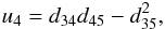 where dij = sitj − sjti. Equivalent expressions for a quartic equation in x can be found by exchanging the indices 1 ↔ 2 and 3 ↔ 5.
Various closed-form solutions of quartic polynomial equations have been published since the first by Cardano (1545) but it appears that no algorithm has been developed that is completely robust when implemented using floating point arithmetic (Herbison-Evans 1994). Instead, ellc uses the rpoly algorithm (Jenkins 1975) followed by “root-polishing” using Laguerre’s algorithm (Press et al. 1992) to ensure that the correct number of real roots is found and to ensure that they are accurate to within the machine floating-point precision. Given the roots of the quartics in x and y, the remaining task is to identify which combinations of these roots correspond to intersections of the ellipses. This proves to be quite problematic because of cases such as those shown in Fig. A.1, which often occur in the calculation of the eclipses for two stars with inclinations close to 90°. These cases also suffer from inaccurate values of the coefficients u0...u4 because of rounding errors. The roots of the quartics will give inaccurate estimates of the positions of any intersections in these cases no matter how good the root-finding algorithm. This makes it extremely difficult to find a robust way to determine if some, none or all of the combinations of roots correspond to actual intersections, tangent points (which I do not consider to be intersections in this context), “near-misses” or spurious solutions of the quartics that correspond to incorrect combinations of x and y.
Most of these problems are the result of the relative orientations of the ellipses, so to find which combinations of x and y correspond to actual intersections the coordinate system is rotated by 45°, the quartic equations for x′ and y′ are solved in the transformed coordinate system, and then apply the inverse transformation to the resulting real roots. Only combinations of x and y that correspond to intersection points or tangent points will appear in the lists of paired real roots calculated for both orientations. Since it is not known a priori which of the two orientations gives reliable results, this analysis is repeated for a third orientation rotated by 60° to the first and search for combinations of x and y that are common to at least two orientations. The resulting list of candidate intersection points is then searched for duplicates with a tolerance of 10-9, which are then removed. If only one candidate intersection point remains then this must be a tangent point. If two unique candidate intersection points are found a simple test of whether the mid-points between these points on the circumference of one ellipse lie inside or outside the other ellipse is sufficient to determine if one ellipse is tangent at two points to the other. A similar test can be used to identify the tangent point in the case of 3 candidate intersection points.
 |
Fig. A.1 The intersection of two ellipses in a configuration that makes the calculation of the intersections difficult using floating point arithmetic. The lower panel shows a sketch of an exaggerated view near the intersection region. The dashed lines show the values of x and y that should be obtained by solving the relevant quartic polynomials. Dots mark the intersection points and open circles mark spurious solutions of both quartics. |
All Tables
All Figures
|
Fig. 1 Coordinate systems used to define the shape and position of each star. The companion is located on the positive x-axis and the angular momentum vector for the orbital motion is parallel to the z-axis. The inclination of the orbital axis to the line of sight is i. The origin of the (u,v,w) coordinate system is at the centre-of-mass of the binary system. Other symbols are defined in the text. |
| In the text | |
|
Fig. 2 Upper panel: light curve for a planet on an eccentric orbit with i = 90° calculated using batman. Upper-middle panel: difference between the light curves calculated using ellc for a spherical planet with the grid sizes indicated and with batman for the case i = 90°. Lower-middle panel: difference between the light curves calculated using ellc with the default grid size for planet described by either a Roche potential or a polytrope with index n = 1.5 and with batman for the case i = 90°. Lower panel: difference between the light curves calculated using ellc with the default grid size and a spherical planet and with batman for an eccentric orbit with i = 87°. The difference in flux of approximately 50 ppm during ingress and egress is the result of an inaccurate estimate for the time of periastron in the batman model. |
| In the text | |
|
Fig. 3 Comparison of the light curves and radial velocity curves for a binary system showing double-partial eclipses computed using Nightfall (dashed lines) and ellc (dotted lines). |
| In the text | |
|
Fig. 4 Comparison of the light curves for a spherical star with two circular spots eclipsed by a spherical dark body calculated using ellc (thin line) and KSint (points). |
| In the text | |
|
Fig. 5 Phase-binned Kepler short-cadence data for KPD 1946+4340 (points) compared to light curves generated using ellc using the Roche potential (solid line) and a polytrope with index n = 1.5 (dashed line). |
| In the text | |
|
Fig. 6 Simulation of the photometric Rossiter-McLaughlin (R-M) effect for a pair of white dwarf stars rotating close to their break-up velocity in an eclipsing binary with a period of 39.1 min. Upper panels: light curve of the binary; the two lower panels: contribution to this light curve due to the photometric R-M effect. In all panels, the solid line is calculated using Roche geometry for stars with rotation axes aligned with the orbital axis and dashed lines are for models of spherical stars with λ = 60°. |
| In the text | |
|
Fig. 7 Light curves of the short-period M-dwarf – white-dwarf binary GD448 simulated using Nightfall and using ellc with two sets of heating/irradiation parameters H0,H1, as indicated, and also using a simplified model of the reflection effect with α = 2.1. |
| In the text | |
|
Fig. 8 Observed light curves for the eclipsing binary J0113+31 (points, Gómez Maqueo Chew et al. 2014) compared to light curves generated using ellc for the parameters shown in Table 1 (solid lines). |
| In the text | |
|
Fig. 9 Parameter correlation plots for my fit using ellc to the radial velocity data and light curves of the eclipsing binary J0113+31 from Gómez Maqueo Chew et al. (2014, GMC+2014). The adopted parameter values from GMC+2014 are indicated by lines/points in each panel. The contours in each panel show the 0.5-, 1-, 1.5- and 2-sigma confidence regions for each joint parameter distributions. Points outside the 2-sigma confidence region are individual steps from the emcee MCMC chain. |
| In the text | |
|
Fig. 10 Observed light curves for the eclipsing binary HD 23642 (points) compared to light curves generated using ellc_emcee.py for the parameters shown in Table 2 (solid lines). |
| In the text | |
|
Fig. 11 Parameter correlation plots for selected parameters from my fit using ellc_emcee to the Kepler K2 light curve of HD 23642. The parameter values from the analysis of David et al. (2016) are indicated by lines/points in each panel. The contours in each panel show the 0.5-, 1-, 1.5- and 2-sigma confidence regions for each joint parameter distributions. Points outside the 2-sigma confidence region are individual steps from the emcee MCMC chain. |
| In the text | |
|
Fig. A.1 The intersection of two ellipses in a configuration that makes the calculation of the intersections difficult using floating point arithmetic. The lower panel shows a sketch of an exaggerated view near the intersection region. The dashed lines show the values of x and y that should be obtained by solving the relevant quartic polynomials. Dots mark the intersection points and open circles mark spurious solutions of both quartics. |
| In the text | |
Current usage metrics show cumulative count of Article Views (full-text article views including HTML views, PDF and ePub downloads, according to the available data) and Abstracts Views on Vision4Press platform.
Data correspond to usage on the plateform after 2015. The current usage metrics is available 48-96 hours after online publication and is updated daily on week days.
Initial download of the metrics may take a while.