| Issue |
A&A
Volume 591, July 2016
|
|
|---|---|---|
| Article Number | A27 | |
| Number of page(s) | 6 | |
| Section | Interstellar and circumstellar matter | |
| DOI | https://doi.org/10.1051/0004-6361/201628395 | |
| Published online | 06 June 2016 | |
Herschel detects oxygen in the β Pictoris debris disk⋆
1
Department of Astronomy, Stockholm University, AlbaNova University
Center, 106 91
Stockholm,
Sweden
e-mail:
This email address is being protected from spambots. You need JavaScript enabled to view it.
2
Instituut voor Sterrenkunde, KU Leuven, Celestijnenlaan 200
D, 3001
Leuven,
Belgium
3
Department of Physics and Astronomy, University College
London, Gower St,
London
WC1E 6BT,
UK
4
Astronomy and Astrophysics Research Group, Dep. of Physics and
Astrophysics, Vrije Universiteit Brussel, Pleinlaan 2, 1050
Brussels,
Belgium
5 Radio Astronomy Laboratory, University of California at
Berkeley, CA 94720, USA
6
ALMA, Alonso de Córdova 3107, Vitacura,
Santiago,
Chile
7
Astronomical Institute Anton Pannekoek, University of
Amsterdam, Kruislaan
403, 1098 SJ
Amsterdam, The
Netherlands
8
Afdeling Sterrenkunde, Radboud Universiteit
Nijmegen, Postbus
9010, 6500 GL
Nijmegen, The
Netherlands
9
National Research Council of Canada, Herzberg Institute of
Astrophysics, 5071 West Saanich
Road, Victoria,
BC, V9E 2E7, Canada
10
Earth and Space Sciences, Chalmers University of
Technology, 412
96
Gothenburg,
Sweden
11
School of Physics and Astronomy, Cardiff University,
Queens Buildings The Parade,
Cardiff
CF24 3AA,
UK
12
Institute of Astronomy, ETH Zurich, 8093
Zurich,
Switzerland
13
UK Astronomy Technology Centre, Royal Observatory
Edinburgh, Blackford
Hill, EH9 3HJ,
UK
14
School of Physics and Astronomy, University of St
Andrews, North Haugh, St.
Andrews, Fife
KY16 9SS,
UK
15
Department of Astronomy, University of Texas, 1 University Station
C1400, Austin,
TX
78712,
USA
16
ESA, Directorate of Science, Scientific Support Office, European
Space Research and Technology Centre (ESTEC/SCI-S), Keplerlaan 1,
2201 AZ
Noordwijk, The
Netherlands
17
Leiden Observatory, Leiden University,
PO Box 9513, 2300 RA
Leiden, The
Netherlands
18
European Southern Observatory, Karl-Schwarzschild-Strasse 2, 85748
Garching,
Germany
19
Institute for Astronomy, University of Edinburgh,
Blackford Hill, Edinburgh
EH9 3HJ,
UK
20
Space Science and Technology Department, Rutherford Appleton
Laboratory, Oxfordshire, OX11
0QX, UK
21
Laboratoire AIM, CEA/DSM-CNRS-Université Paris Diderot,
IRFU/Service d’Astrophysique, Bat. 709, CEA-Saclay, 91191
Gif-sur-Yvette Cedex,
France
22
SRON Netherlands Institute for Space Research,
PO Box 800, 9700 AV
Groningen, The
Netherlands
Received: 26 February 2016
Accepted: 25 April 2016
Abstract
The young star β Pictoris is well known for its dusty debris disk produced through collisional grinding of planetesimals, kilometre-sized bodies in orbit around the star. In addition to dust, small amounts of gas are also known to orbit the star; this gas is likely the result of vaporisation of violently colliding dust grains. The disk is seen edge on and from previous absorption spectroscopy we know that the gas is very rich in carbon relative to other elements. The oxygen content has been more difficult to assess, however, with early estimates finding very little oxygen in the gas at a C/O ratio that is 20 × higher than the cosmic value. A C/O ratio that high is difficult to explain and would have far-reaching consequences for planet formation. Here we report on observations by the far-infrared space telescope Herschel, using PACS, of emission lines from ionised carbon and neutral oxygen. The detected emission from C+ is consistent withthat previously reported observed by the HIFI instrument on Herschel, while the emission from O is hard to explain without assuming a higher density region in the disk, perhaps in the shape of a clump or a dense torus required to sufficiently excite the O atoms. A possible scenario is that the C/O gas is produced by the same process responsible for the CO clump recently observed by the Atacama Large Millimeter/submillimeter Array in the disk and that the redistribution of the gas takes longer than previously assumed. A more detailed estimate of the C/O ratio and the mass of O will have to await better constraints on the C/O gas spatial distribution.
Key words: stars: early-type / stars: individual: beta Pictoris / circumstellar matter
Herschel is an ESA space observatory with science instruments provided by European-led Principal Investigator consortia and with important participation from NASA.
© ESO, 2016
1. Introduction
The star β Pictoris is young (23 ± 3 Myr; Mamajek & Bell 2014), nearby (19 pc; van Leeuwen 2007), and harbours a large debris disk, making it a target of intense scrutiny since its discovery by the infrared astronomical satellite IRAS in 1984 (Aumann 1985). As the survival time for dust grains in the disk is far shorter than the age of the system, it was argued early on that the dust must be replenished through collisional fragmentation of larger bodies, hence the name “debris disk” (Backman & Paresce 1993). The interest in the β Pic disk is strongly linked to the interest in planet formation; the disk was discovered a decade before the first exoplanets, yet is apparently the result of the same mechanisms that form planets and, therefore, provides a valuable example to test theory. Rocky planets, such as the Earth, are generally believed to be built up by smaller bodies called planetesimals, which range in size from 1 kilometre to hundreds of kilometres (Nagasawa et al. 2007). How the planetesimals are built up, in turn, is one of the outstanding problems of planet formation theory today. One of the more promising suggestions to answer this problem is production through a “streaming instability” (Johansen et al. 2007).
Why some stars seem to form planets while others may not is still not understood, but one clue could be the observed correlation between planet incidence and the elemental abundances of the parent star; stars of higher heavy element abundance are argued to be more likely to have massive planets (Fischer & Valenti 2005; Buchhave et al. 2014). If the composition of the star reflects the composition of the planet-forming disk, one explanation could be that the dust grains that eventually build up the planetesimals are more easily formed in an environment enriched in heavier elements. The picture is far from clear, however, since a correlation with host star metallicity is observed for gas giants, but not for small exoplanets (Buchhave et al. 2014) or for the tracers of planetesimal formation known as debris disks (Greaves et al. 2006; Wyatt et al. 2007; Moro-Martín et al. 2015).
The β Pic system has passed its planetesimal formation phase and today we observe a resulting planetesimal belt located at a radial distance of 100 au (Thébault & Augereau 2007; Wilner et al. 2011; Dent et al. 2014) and a recently discovered massive planet (10–12 times the mass of Jupiter) on a ~9 au orbit (Lagrange et al. 2010; Millar-Blanchaer et al. 2015). In addition to the dust produced through a collisional cascade originating from the planetesimals, we also observe gas in the system (Hobbs et al. 1985; Olofsson et al. 2001; Roberge et al. 2006, hereafter ROB06). With an estimated total mass that is just a fraction of an Earth mass (Zagorovsky et al. 2010, hereafter ZBW10), this gas is far too tenuous to contribute to the formation of new planets. Instead, it is thought to be the result of the reverse process: vaporisation of colliding dust grains originating in the planetesimals (Liseau & Artymowicz 1998; Czechowski & Mann 2007). Alternatively, the gas could also be released from the dust through photo-desorption (Chen et al. 2007; Grigorieva et al. 2007) or collisions between volatile-rich comets in a massive Kuiper-belt analogue (Zuckerman & Song 2012). The latter seems favoured by recent Atacama Large Millimeter/submillimeter Array (ALMA) observations of CO apparently released from a clump located at 85 au, where an enhanced collision rate induced by either a resonance trap from a migrating planet or a residue from a former giant collision are suggested as possible mechanisms (Dent et al. 2014; Jackson et al. 2014). Given the rapid dissociation time for CO in this environment (120 yr; Visser et al. 2009), it is clear that the gas must be currently produced and that it is a source of both C and O.
The long-standing puzzle of how gas could be kept in the disk while subject to a strong radiation force from the star was resolved by the discovery of a large overabundance of carbon with respect to detected metallic elements in the disk gas (e.g. Na, Fe, and Ca; ROB06) acting as a braking agent (Fernández et al. 2006). The overabundance is not necessarily a consequence of the dust grains being unusually carbon rich, it could also be due to chemical differentiation through preferential removal of the observed metallic elements (Xie et al. 2013). In contrast to carbon, the metallic elements experience a strong radiation force from the star, up to a few hundred times stronger than the gravitational force. Oxygen, on the other hand, is similar to carbon in that it is not affected by radiation pressure from the star (Fernández et al. 2006) and is thus expected to be closely mixed with carbon. It was therefore surprising when absorption spectroscopy found a C/O ratio that is 20 × higher than the cosmic abundance found in the Sun and 100 × the ratio found in carbonaceous chondrite meteorites (ROB06).
The C/O ratio is believed to strongly affect the outcome of the planet formation process (Kuchner & Seager 2005). For example, the sequence by which elements condense as the gas cools, and thus the mass distribution and planet formation efficiency, changes significantly with the C/O ratio. A ratio larger than 0.8 would result in carbide-dominated interiors of planets (Bond et al. 2010) as opposed to the silicate-dominated composition found in the rocky planets of our solar system. An example of an extra-solar planet where a super-cosmic C/O ratio has been suggested is WASP-12b, where a C/O ratio that is already 2 × higher in its atmosphere results in dramatically different mixing ratios of molecular species (Madhusudhan et al. 2011). If the C/O ratio of the disk gas reflects the composition of the β Pic planet and the C/O ratio is indeed higher than the cosmic ratio by a factor 20, then the planet would likely have a diamond core and be evidence for a very exotic planet formation scenario (Kuchner & Seager 2005). The evolutionary and atmospheric models used to estimate the mass of the planet from photometry would be invalid (Lagrange et al. 2010; Baraffe et al. 2003) and would have to be replaced with alternative, high-C/O models. Determining the relative abundance of C and O is thus highly relevant for understanding the available paths for planet formation. We present observations of C ii and O i obtained using the far-infrared space telescope Herschel that aim to facilitate an estimate of the O mass and C/O ratio of the gas in the β Pic debris disk.
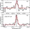 |
Fig. 1 Emission lines observed from β Pic with fitted Gaussian profiles overplotted. The spectra were continuum subtracted and rebinned. The vertical dashed line shows the expected wavelength of the emission line. The measured fluxes are reported in Table 1. a): [O i] 63.2 μm emission line observed by the central spaxel (12) of PACS. The wavelength scale is in the local standard of rest frame. b): [C ii] 157.7 μm emission line of the central spaxel. The unbroken vertical line shows the fitted centre of the emission line. |
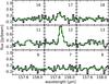 |
Fig. 2 Central 3 × 3 spaxels of the 5 × 5 PACS array, showing the detected [C ii] 157.7 μm emission line. Spaxels outside this region show no signal. In addition to the central spaxel 12, the adjacent spaxels 11, 13, and 17 also detect a signal (listed in Table 1). Overplotted on the data are synthetic observations of the disk model “5 × 5 au” (Sect. 3.2, Table 2). |
2. Observations
The data presented are part of the Herschel guaranteed time Stellar Disk Evolution key programme (PI Olofsson; OBSIDs 1342188425 and 1342198171, observed on 2009-12-22 [O i] and 2010-06-02 [C ii], respectively). We used the Photodetector Array Camera and Spectrometer (PACS; Poglitsch et al. 2010) on board the Herschel Space Observatory (Pilbratt et al. 2010), operating as an integral field spectrometer to observe β Pic in the 158 μm [C ii] and 63 μm [O i] line regions. The [O i] 63 μm line was observed with a dedicated PACS chop/nod line spectroscopy observation centred on the line, while the [C ii] 158 μm line was extracted from a deep observation of the entire PACS wavelength range. Both lines were detected in emission (Fig. 1), but are unresolved at the 86 km s-1 (at 63 μm) and 239 km s-1 (at 158 μm) per resolution channel of PACS. Since the field is spatially resolved into 5 × 5 spaxels (i.e. spectral pixels, each of side 9.4′′), we can clearly see that the emission is centred on the star and not due to an offset background object (Fig. 2).
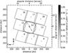 |
Fig. 3 Central 3 × 3 spaxels of the 5 × 5 PACS array, showing the coverage of a modelled disk (model “5 × 5 au”) and location of the star with respect to the spaxel coordinates. The central position of each spaxel is indicated with a plus sign and the position of β Pic at the epoch of the observation with a star. The dashed circle corresponds to the 11′′ FWHM of the beam at 158 μm. |
Figure 3 shows the orientation of the spaxels with respect to β Pic in the case of the C ii observations. The telescope pointing model indicates that the central spaxel was offset from β Pic by 1.0′′ for the C ii and 0.8′′ for the O i observations. The typical 68% confidence pointing accuracy for Herschel at these epochs were ~2′′ (Sánchez-Portal et al. 2014).
The data reduction was essentially carried out as described in Cataldi et al. (2015). We used the “background normalisation” pipeline script within the Herschel interactive processing environment (HIPE) version 14.0 (Ott 2010). This pipeline uses the background emission from the telescope itself to background subtract and calibrate the data. The data were binned into a wavelength grid by setting oversample = 4 (increasing the spectral sampling) and upsample = 1 (keeping neighbouring data points uncorrelated). The continuum was subtracted by fitting linear polynomials to the spectra with the line region masked. We used the pipeline-generated noise estimate “stddev” as relative weights for the continuum fit. This is particularly important for the O i spectra, where the noise is smallest at the line centre and increases towards the spectral edges. Finally, we estimated the noise for each spaxel individually. To this end, we computed the standard deviation within two spectral windows placed sufficiently far from the line centre to avoid any contamination by line emission. The width of each window was chosen equal to 2.5× the spectral resolution of PACS (i.e. 2.5× the full width at half maximum (FWHM) of an unresolved line).
We fit a Gaussian function to the spectra to measure the line flux, where the FWHM of the Gaussian was fixed to the FWHM of the line-spread function (i.e. the spectral resolution). The central wavelength of the Gaussian was also generally fixed to the expected wavelength corrected for the known radial velocity of β Pic (Brandeker 2011). An exception was the central spaxel of the C ii observations, where it is apparent by eye that there is a shift between the centre of the emission line and the expected central wavelength (Fig. 1). In this case we let the line centre be a free parameter and found the line centre to be redshifted by 0.02 μm. This shift is within specification of the PACS wavelength calibration and would be expected for an off-centre point source (PACS observer’s manual v.2.5.1, HERSCHEL-HSC-DOC-0832, Sect. 4.7.2).
In order to estimate the error on the measured line flux, we produced 105 fits, including the continuum fit and subtraction, to resampled data for each spaxel with detected line emission. The resampling is achieved by adding normally distributed noise with a standard deviation according to the previously determined error of the spectrum with the line centre and FWHM fixed. The error on the flux is then estimated as the standard deviation of the resulting distribution of fitted fluxes.
PACS detected emission from the β Pic gas disk.
3. Results and analysis
3.1. Detected emission
The [C ii] emission detected by Herschel/PACS from β Pic (Table 1) is ~30% lower than the corresponding emission detected by Herschel/HIFI ((2.4 ± 0.1) × 10-14 erg s-1 cm-2 beam-1; Cataldi et al. 2014), and a factor of three below the tentative detection by the Infrared Space Observatory (Kamp et al. 2003). The difference in the observed flux between PACS and HIFI may be due to slight pointing differences, as the source is likely to be marginally resolved by a 11′′ beam; the precise pointing could thus be important. However, by varying the pointing centre by a few arcseconds (the expected pointing accuracy) in synthetic observations of our models, we found a difference of at most a few percent. This could be because our assumed angular flux distribution is wrong (e.g. the real distribution is not symmetric between the north-east [NE] and south-west [SW]) and/or because the pointing offset between the observations is higher than assumed. It could also be due to an absolute calibration issue, which is expected to be 12% but indeed could be off by up to 30% (PACS observer’s manual v.2.5.1, Sect. 4.10.2.1). Finally, the difference could also be because the beams of PACS and HIFI are not identical.
Oxygen has not previously been observed in emission, but a model of the β Pic gas disk by ZBW10 predicted a flux 3 orders of magnitude below the detected level. They assumed a spatial distribution of well-mixed gas derived from observations of Na i (Brandeker et al. 2004) with only C overabundant (by a factor of 20, ROB06). Cataldi et al. (2014) used the HIFI observations of [C ii] 158 μm to update the ZBW10 model and found that a C overabundance by a factor of 300 was required to explain the strong emission observed, assuming a well-mixed gas. To test how the observed [O i] 63 μm emission constrains the mass and distribution of O, we produced a range of models assuming different spatial distributions and abundances of the gas, as reported in Sect. 3.2 below.
3.2. Gas disk models
To model the gas emission from the β Pic disk we used the ontario code, specifically developed for modelling gas in debris disks around A–F stars (ZBW10). Given the input parameters, which are the stellar spectrum and spatial distribution of dust and gas (including its abundance), ontario computes the thermal and ionisation balance of the gas and then the statistical equilibrium population of energy levels in species of interest, including their emitted spectra. This is in particular important for O that, in contrast to C, has level populations that generally are out of local thermal equilibrium (LTE) in the low electron density environment of the disk gas; we find the critical electron densities at 100 K for C ii and O i to be 6 cm-3 and 2.5 × 105 cm-3, respectively. Moreover, the [O i] 63 μm line, like [C ii] 158 μm, becomes optically thick at column densities of ~5 × 1017 cm-2 (assuming a line width of 2 km s-1). The line luminosities of the disk thus not only depend on the gas mass, but also depend strongly on the spatial distribution of the gas. Since the [C ii] 158 μm and [O i] 63 μm lines are also important cooling lines, we updated the thermal and statistical equilibrium solution in ontario to approximate the radiative transfer effect using photon escape probabilities, essentially following Appendix B of Tielens & Hollenbach (1985). We start by computing the level populations for the innermost grid points and then continue outwards while adjusting for the extinction from interior grid points towards the star. As a second-order correction, we take into account locally scattered photons using a photon escape formulation. The photon escape fraction is computed iteratively starting with an assumption of complete escape and then using the computed level population from the previous iteration to approximate the photon escape probability from the average of four directions (in, out, up, and down, as described in Gorti & Hollenbach 2004), obtaining a new level population. Once the level populations of each grid point are defined, the radiative transfer equation is integrated along the line of sight from the observer, assuming a Keplerian velocity field to produce an angular distribution of the spectral profile, as described in Cataldi et al. (2014).
Model properties.
3.2.1. The assumed spatial distribution of gas
If C and O are produced principally from the enhanced collision rate responsible for the production of CO observed by ALMA at an orbital radius of ~85 au (Dent et al. 2014), then one would expect the gas distribution to peak at 85 au and diffuse to other regions of the disk. Given that the CO molecule is short lived (~120 yr at 85 au) while C and O in their ion or atomic form are stable, we would expect C and O to be more evenly distributed than CO, perhaps in a ring slowly diffusing away from the production orbital radius. If, however, the C and O are primarily produced by the same mechanism that is responsible for the observed metallic species in the disk (Na, Fe, Ca, etc., Brandeker et al. 2004), then one could expect the C and O spatial distribution to more closely follow the gas distribution inferred from the spatially resolved Fe i emission (Nilsson et al. 2012) with the density ![Mathematical equation: \begin{equation} \label{eq:Fe_distr} n(r,z) = n_0\left[\frac{2}{(r/r_0)^{2\alpha}+(r/r_0)^{2\beta}}\right]^{1/2} \exp\left[-\left(\frac{z}{h(r)}\right)^{\gamma}\right], \end{equation}](/articles/aa/full_html/2016/07/aa28395-16/aa28395-16-eq66.png) (1)where h(r) = h0(r/r0)δ and the parameters n0, h0, r0, α, β, γ, and δ are as listed in Table 3 of Nilsson et al. (2012). One important parameter missing from Eq. (1) is the inner truncation radius of the disk, since the density n(r,z) diverges as r → 0. Unfortunately, this parameter is difficult to assess because of scattered light residuals from the nearby star dominating the noise inside 2′′ (40 au) in the Nilsson et al. (2012) observations. With VLT/UVES, Brandeker et al. (2004) were able to trace the Na i and Fe i a bit further in to the limit of the observations at 0.7′′ (13 au) from the star. They found an asymmetry in that the disk on the NE side appears to rise in brightness all the way in, while the SW side shows a significant decrease in density inside 36 au.
(1)where h(r) = h0(r/r0)δ and the parameters n0, h0, r0, α, β, γ, and δ are as listed in Table 3 of Nilsson et al. (2012). One important parameter missing from Eq. (1) is the inner truncation radius of the disk, since the density n(r,z) diverges as r → 0. Unfortunately, this parameter is difficult to assess because of scattered light residuals from the nearby star dominating the noise inside 2′′ (40 au) in the Nilsson et al. (2012) observations. With VLT/UVES, Brandeker et al. (2004) were able to trace the Na i and Fe i a bit further in to the limit of the observations at 0.7′′ (13 au) from the star. They found an asymmetry in that the disk on the NE side appears to rise in brightness all the way in, while the SW side shows a significant decrease in density inside 36 au.
The Cataldi et al. (2014)Herschel/HIFI spectrally resolved observations of the [C ii] 158 μm emission line indirectly put constraints on the C spatial distribution under the assumption of a Keplerian rotating disk.They found that the observations were best fit if the gas distribution inferred from Fe i had an inner truncation radius between 30 and 100 au. Indeed, a single torus of radius ~100 au could by itself reasonably fit the data (see Fig. 4 in Cataldi et al. 2014).
Since the constraint on the mass of C and O in the disk depends on the assumed spatial distributions of the gas, we explore the following different reasonable configurations:
-
1.
A C/O gas that is well mixed with the observed Fe and Nadistribution, using Eq. (1) with parameters fit fromNilsson et al. (2012), C/Oabundances as free parameters, and the inner truncation radius at5 au and 35 au (labelling themodels “>5 au” and “>35 au”).
-
2.
Assuming C and O are produced from CO independently from Fe/Na, we use a torus of radius 85 au with a selection of assumed widths and scale heights, motivated by the ALMA CO observations. The model tori have scale heights that are equivalent to their radial extents with the FWHM of 1 au, 5 au, and 10 au, according to a Gaussian distribution with the peak density of C and O as free parameters. The models are labelled “1 × 1 au”, “5 × 5 au”, and “10 × 10 au”, respectively.
The principal purpose of these models is not to accurately model the real spatial distribution of the gas, which indeed likely departs from the assumed cylindrical symmetry implied here. The purpose is instead to study how the predicted emission is influenced by assumptions on the spatial distribution and abundance of gas to help us distinguish between possible scenarios. To make a realistic model of the C and O gas, their spatial distribution would have to be better constrained. Properties of the models are listed in Table 2.
3.2.2. Comparing models to observation
To compare the models with data, we computed a grid of models, deriving the corresponding angular distribution of line luminosity in the sky (as in Cataldi et al. 2014) and then used synthetic PACS observations (as described in Cataldi et al. 2015, but with the updated v6 of the PACS spectrometer beams) to produce a model spectrum for each spaxel to be compared with the observed data. Figure 2 shows the central 3 × 3 spaxels of one such model overplotted on the observed [C ii] 158 μm emission.
We found it challenging to reproduce the detected [O i] 63 μm emission while at the same time maintaining consistency with the observed [C ii] 158 μm emission. Under the assumption that C and O is mixed together well, most spatial distributions tend to underproduce the 63 μm line in comparison to the 158 μm emission. The complication arises from the complex interplay between the heating/cooling, excitation mechanisms and optical thickness effects. Increasing the O abundance increases the cooling, but only until the dominant 63 μm cooling line becomes optically thick. Increasing the abundance even further may then decrease the energy output in the 63 μm line, as locations with lower electron density become optically thick and block the radiation. We thus find that there is a C/O ratio that maximises the 63 μm flux for a fixed 158 μm flux, and this maximum 63 μm flux was below the observed flux for a range of models we tested. For the five different spatial distributions we considered (listed in Table 2), we varied the C and O abundances freely, but filtered out any model that gave a synthetic [C ii] 158 μm flux that differed more than 5% from the observations. We then picked the model that comes closest to reproduce the [O i] 63 μm emission. Only the densest 1 × 1 au model is able to fully reproduce the 63 μm line, while other models underpredict the emission by a factor 2.5–51 (Table 2).
Another problem with the models presented in Table 2 is that the implied column density against the star is orders of magnitude larger than the column densities observed by FUSE (ROB06), which are NO i = (3−8) × 1015 cm-2, NC i = (2−4) × 1016 cm-2, and NC ii = (1.6−4.1) × 1016 cm-2. As discussed by Brandeker (2011), part of the difference could be due to the difficulties in measuring unresolved optically thick lines. In ROB06, a single broad component was assumed for an O i absorption line (broadening parameter b = 15 km s-1), which effectively gives a lower limit on the column density. If instead a narrow component is assumed, say b = 1−2 km s-1, the column density could be much higher (in excess of NO i = 1017 cm-2) and still be consistent with the observed line profile (see supplementary Fig. 1 of Roberge et al. 2006). The lower C i column density is harder to explain in this way, since it is based on a robust measurement of the  state, where an optically thin line was observed by STIS (Roberge et al. 2000). We conclude that the absorption measurements are consistent with a low C/O ratio gas (≲ 1) in a non-cylindrically symmetric distribution.
4. Discussion
From the modelling described in the previous section we conclude that we can only explain the observed 63 μm emission if there is a region in the gas disk that is sufficiently dense to effectively excite O, meaning an electron density ne ≳ 2.5 × 104 cm-3, the critical density for the [O i] 63 μm line. This region does not have to be very large, however; if optically thick, in LTE, and with temperatures in the range 80–100 K, a high-density clump with a diameter of a few au would be sufficient to produce the observed emission. Such a clump would show up in the angular distribution of [C ii] 158 μm and in particular in [C i]. Considering the clump recently imaged in CO by ALMA (Dent et al. 2014), perhaps there is a corresponding clump in the C and O distribution that would explain the enhanced [O i] 63 μm emission. The [C ii] 158 μm spectral profile by HIFI also seems to be consistent with a C clump to the SW (see Fig. 6 of Cataldi et al. 2014). A clumpy distribution may thus be preferred by observations, but this is in contrast to the expectation outlined in Sect. 3.2.1, that C and O would have diffused into a smooth distribution because they have a much longer lifetime than CO. This could be resolved if the diffusion process is slower than anticipated (α ≲ 0.01, resulting in a viscous timescale ≳Myr; Xie et al. 2013) so that the pattern imprinted by the CO distribution lasts longer or if the event producing CO is recent (≪Myr). More detailed models are required to evaluate whether these scenarios are credible.
A region of enhanced electron density to the SW might be able to explain another puzzling property of the β Pic disk; why the asymmetry between the NE and SW is so pronounced in Na i and Fe i (see Figs. 2 and 3 of Brandeker et al. 2004). With an increased electron density, the neutral fractions of Na i and Fe i would dramatically rise because of more frequent recombination, meaning that any given particle would spend a longer time in its neutral state. Since the radiation force on the neutral species of Fe and Na is much stronger than gravity (27× and 360×, respectively) and only the ionised species are effectively braked by Coulomb interaction with the C+ gas (Fernández et al. 2006), the atoms are removed from the system with a drift velocity νdrift = νionf, where νion is the average velocity the atom reaches before ionisation and subsequent braking by the C+ gas, and f is the fraction of the time the particle spends in its neutral state. For Fe, νion = 0.5 km s-1 and for Na, νion = 3.3 km s-1 (Brandeker 2011).
The spatial distribution of C and O is presently not constrained enough to be able to derive an accurate O mass. If the C and O are indeed produced by outgassing and subsequent dissociation of molecules from colliding comets, as suggested by Zuckerman & Song (2012) and Dent et al. (2014), then the expected C/O ratio would be 0.1–1, depending on the fraction of CO/H2O present in the comet-like bodies. See also Kral et al. (2016) for a detailed attempt to model C and O in the disk as a result of CO dissociation. Upcoming ALMA observations of the [C i] 609 μm line should be able to settle the case.
5. Conclusions
In summary, we find that Herschel/PACS observations of [O i] 63 μm and [C ii] 158 μm emission from β Pic result in the following conclusions:
-
1.
Emission from C ii and O iwas detected from β Pic.
-
2.
The detected emission from [O i] 63 μm is much stronger than expected from cylindrically symmetric models.
-
3.
A region of relatively high density, perhaps in a clump similar to that observed in CO, is required to explain the [O i] 63 μm emission.
-
4.
To derive a reliable mass of O, and thereby constrain the C/O ratio of the disk, knowing the spatial distribution of C and O is essential.
We expect that [C i] 609 μm observations by ALMA will be able to constrain the spatial distribution of C, and thereby the electron density and C/O ratio.
Acknowledgments
We thank Aki Roberge, Philippe Thébault, and Yanqin Wu for helpful discussions. A.B. was supported by the Swedish National Space Board (contract 75/13). B.A. was a Postdoctoral Fellow of the Fund for Scientific Research, Flanders. R.J.I. acknowledges support from ERC in the form of the Advanced Investigator Programme, 321302, COSMICISM. PACS has been developed by a consortium of institutes led by MPE (Germany) and including UVIE (Austria); KU Leuven, CSL, IMEC (Belgium); CEA, LAM (France); MPIA (Germany); INAF-IFSI/OAA/OAP/OAT, LENS, SISSA (Italy); IAC (Spain). This development has been supported by the funding agencies BMVIT (Austria), ESA-PRODEX (Belgium), CEA/CNES (France), DLR (Germany), ASI/INAF (Italy), and CICYT/MCYT (Spain).
References
- Aumann, H. H. 1985, PASP, 97, 885 [NASA ADS] [CrossRef] [Google Scholar]
- Backman, D. E., & Paresce, F. 1993, in Protostars and Planets III, eds. E. H. Levy, & J. I. Lunine, 1253 [Google Scholar]
- Baraffe, I., Chabrier, G., Barman, T. S., Allard, F., & Hauschildt, P. H. 2003, A&A, 402, 701 [NASA ADS] [CrossRef] [EDP Sciences] [Google Scholar]
- Bond, J. C., O’Brien, D. P., & Lauretta, D. S. 2010, ApJ, 715, 1050 [NASA ADS] [CrossRef] [Google Scholar]
- Brandeker, A. 2011, ApJ, 729, 122 [NASA ADS] [CrossRef] [Google Scholar]
- Brandeker, A., Liseau, R., Olofsson, G., & Fridlund, M. 2004, A&A, 413, 681 [NASA ADS] [CrossRef] [EDP Sciences] [Google Scholar]
- Buchhave, L. A., Bizzarro, M., Latham, D. W., et al. 2014, Nature, 509, 593 [NASA ADS] [CrossRef] [Google Scholar]
- Cataldi, G., Brandeker, A., Olofsson, G., et al. 2014, A&A, 563, A66 [NASA ADS] [CrossRef] [EDP Sciences] [Google Scholar]
- Cataldi, G., Brandeker, A., Olofsson, G., et al. 2015, A&A, 574, L1 [NASA ADS] [CrossRef] [EDP Sciences] [Google Scholar]
- Chen, C. H., Li, A., Bohac, C., et al. 2007, ApJ, 666, 466 [NASA ADS] [CrossRef] [Google Scholar]
- Czechowski, A., & Mann, I. 2007, ApJ, 660, 1541 [NASA ADS] [CrossRef] [Google Scholar]
- Dent, W. R. F., Wyatt, M. C., Roberge, A., et al. 2014, Science, 343, 1490 [Google Scholar]
- Fernández, R., Brandeker, A., & Wu, Y. 2006, ApJ, 643, 509 [NASA ADS] [CrossRef] [Google Scholar]
- Fischer, D. A., & Valenti, J. 2005, ApJ, 622, 1102 [NASA ADS] [CrossRef] [Google Scholar]
- Gorti, U., & Hollenbach, D. 2004, ApJ, 613, 424 [NASA ADS] [CrossRef] [Google Scholar]
- Greaves, J. S., Fischer, D. A., & Wyatt, M. C. 2006, MNRAS, 366, 283 [NASA ADS] [CrossRef] [Google Scholar]
- Grigorieva, A., Thébault, P., Artymowicz, P., & Brandeker, A. 2007, A&A, 475, 755 [NASA ADS] [CrossRef] [EDP Sciences] [Google Scholar]
- Hobbs, L. M., Vidal-Madjar, A., Ferlet, R., Albert, C. E., & Gry, C. 1985, ApJ, 293, L29 [NASA ADS] [CrossRef] [Google Scholar]
- Jackson, A. P., Wyatt, M. C., Bonsor, A., & Veras, D. 2014, MNRAS, 440, 3757 [NASA ADS] [CrossRef] [Google Scholar]
- Johansen, A., Oishi, J. S., Mac Low, M.-M., et al. 2007, Nature, 448, 1022 [Google Scholar]
- Kamp, I., van Zadelhoff, G.-J., van Dishoeck, E. F., & Stark, R. 2003, A&A, 397, 1129 [NASA ADS] [CrossRef] [EDP Sciences] [Google Scholar]
- Kral, Q., Wyatt, M. C., Carswell, R. F., et al. 2016, MNRAS, submitted [Google Scholar]
- Kuchner, M. J., & Seager, S. 2005, ArXiv e-prints [arXiv:astro-ph/0504214] [Google Scholar]
- Lagrange, A.-M., Bonnefoy, M., Chauvin, G., et al. 2010, Science, 329, 57 [NASA ADS] [CrossRef] [PubMed] [Google Scholar]
- Liseau, R., & Artymowicz, P. 1998, A&A, 334, 935 [NASA ADS] [Google Scholar]
- Lodders, K. 2003, ApJ, 591, 1220 [NASA ADS] [CrossRef] [Google Scholar]
- Madhusudhan, N., Harrington, J., Stevenson, K. B., et al. 2011, Nature, 469, 64 [NASA ADS] [CrossRef] [PubMed] [Google Scholar]
- Mamajek, E. E., & Bell, C. P. M. 2014, MNRAS, 445, 2169 [NASA ADS] [CrossRef] [Google Scholar]
- Millar-Blanchaer, M. A., Graham, J. R., Pueyo, L., et al. 2015, ApJ, 811, 18 [Google Scholar]
- Moro-Martín, A., Marshall, J. P., Kennedy, G., et al. 2015, ApJ, 801, 143 [NASA ADS] [CrossRef] [Google Scholar]
- Nagasawa, M., Thommes, E. W., Kenyon, S. J., Bromley, B. C., & Lin, D. N. C. 2007, Protostars and Planets V, 639 [Google Scholar]
- Nilsson, R., Brandeker, A., Olofsson, G., et al. 2012, A&A, 544, A134 [NASA ADS] [CrossRef] [EDP Sciences] [Google Scholar]
- Olofsson, G., Liseau, R., & Brandeker, A. 2001, ApJ, 563, L77 [NASA ADS] [CrossRef] [EDP Sciences] [Google Scholar]
- Ott, S. 2010, in Astronomical Data Analysis Software and Systems XIX, eds. Y. Mizumoto, K.-I. Morita, & M. Ohishi, ASP Conf. Ser., 434, 139 [Google Scholar]
- Pilbratt, G. L., Riedinger, J. R., Passvogel, T., et al. 2010, A&A, 518, L1 [CrossRef] [EDP Sciences] [Google Scholar]
- Poglitsch, A., Waelkens, C., Geis, N., et al. 2010, A&A, 518, L2 [NASA ADS] [CrossRef] [EDP Sciences] [Google Scholar]
- Roberge, A., Feldman, P. D., Lagrange, A. M., et al. 2000, ApJ, 538, 904 [NASA ADS] [CrossRef] [Google Scholar]
- Roberge, A., Feldman, P. D., Weinberger, A. J., Deleuil, M., & Bouret, J.-C. 2006, Nature, 441, 724, (ROB06) [NASA ADS] [CrossRef] [PubMed] [Google Scholar]
- Sánchez-Portal, M., Marston, A., Altieri, B., et al. 2014, Exp. Astron., 37, 453 [NASA ADS] [CrossRef] [Google Scholar]
- Thébault, P., & Augereau, J.-C. 2007, A&A, 472, 169 [NASA ADS] [CrossRef] [EDP Sciences] [Google Scholar]
- Tielens, A. G. G. M., & Hollenbach, D. 1985, ApJ, 291, 747 [NASA ADS] [CrossRef] [Google Scholar]
- van Leeuwen, F. 2007, A&A, 474, 653 [NASA ADS] [CrossRef] [EDP Sciences] [Google Scholar]
- Visser, R., van Dishoeck, E. F., & Black, J. H. 2009, A&A, 503, 323 [NASA ADS] [CrossRef] [EDP Sciences] [Google Scholar]
- Wilner, D. J., Andrews, S. M., & Hughes, A. M. 2011, ApJ, 727, L42 [NASA ADS] [CrossRef] [Google Scholar]
- Wyatt, M. C., Smith, R., Su, K. Y. L., et al. 2007, ApJ, 663, 365 [NASA ADS] [CrossRef] [Google Scholar]
- Xie, J.-W., Brandeker, A., & Wu, Y. 2013, ApJ, 762, 114 [NASA ADS] [CrossRef] [Google Scholar]
- Zagorovsky, K., Brandeker, A., & Wu, Y. 2010, ApJ, 720, 923 (ZBW10) [NASA ADS] [CrossRef] [Google Scholar]
- Zuckerman, B., & Song, I. 2012, ApJ, 758, 77 [NASA ADS] [CrossRef] [Google Scholar]
All Tables
All Figures
|
Fig. 1 Emission lines observed from β Pic with fitted Gaussian profiles overplotted. The spectra were continuum subtracted and rebinned. The vertical dashed line shows the expected wavelength of the emission line. The measured fluxes are reported in Table 1. a): [O i] 63.2 μm emission line observed by the central spaxel (12) of PACS. The wavelength scale is in the local standard of rest frame. b): [C ii] 157.7 μm emission line of the central spaxel. The unbroken vertical line shows the fitted centre of the emission line. |
| In the text | |
|
Fig. 2 Central 3 × 3 spaxels of the 5 × 5 PACS array, showing the detected [C ii] 157.7 μm emission line. Spaxels outside this region show no signal. In addition to the central spaxel 12, the adjacent spaxels 11, 13, and 17 also detect a signal (listed in Table 1). Overplotted on the data are synthetic observations of the disk model “5 × 5 au” (Sect. 3.2, Table 2). |
| In the text | |
|
Fig. 3 Central 3 × 3 spaxels of the 5 × 5 PACS array, showing the coverage of a modelled disk (model “5 × 5 au”) and location of the star with respect to the spaxel coordinates. The central position of each spaxel is indicated with a plus sign and the position of β Pic at the epoch of the observation with a star. The dashed circle corresponds to the 11′′ FWHM of the beam at 158 μm. |
| In the text | |
Current usage metrics show cumulative count of Article Views (full-text article views including HTML views, PDF and ePub downloads, according to the available data) and Abstracts Views on Vision4Press platform.
Data correspond to usage on the plateform after 2015. The current usage metrics is available 48-96 hours after online publication and is updated daily on week days.
Initial download of the metrics may take a while.