| Issue |
A&A
Volume 591, July 2016
|
|
|---|---|---|
| Article Number | A78 | |
| Number of page(s) | 9 | |
| Section | The Sun | |
| DOI | https://doi.org/10.1051/0004-6361/201628096 | |
| Published online | 20 June 2016 | |
Photospheric and coronal magnetic fields in six magnetographs
I. Consistent evolution of the bashful ballerina
ReSoLVE Centre of Excellence, Space Climate research unit, University of
Oulu,
PO Box 3000,
90014
Oulu,
Finland
e-mail: ilpo.virtanen@oulu.fi; kalevi.mursula@oulu.fi
Received: 8 January 2016
Accepted: 1 April 2016
Aims. We study the long-term evolution of photospheric and coronal magnetic fields and the heliospheric current sheet (HCS), especially its north-south asymmetry. Special attention is paid to the reliability of the six data sets used in this study and to the consistency of the results based on these data sets.
Methods. We use synoptic maps constructed from Wilcox Solar Observatory (WSO), Mount Wilson Observatory (MWO), Kitt Peak (KP), SOLIS, SOHO/MDI, and SDO/HMI measurements of the photospheric field and the potential field source surface (PFSS) model.
Results. The six data sets depict a fairly similar long-term evolution of magnetic fields and the heliospheric current sheet, including polarity reversals and hemispheric asymmetry. However, there are time intervals of several years long, when first KP measurements in the 1970s and 1980s, and later WSO measurements in the 1990s and early 2000s, significantly deviate from the other simultaneous data sets, reflecting likely errors at these times. All of the six magnetographs agree on the southward shift of the heliospheric current sheet (the so-called bashful ballerina phenomenon) in the declining to minimum phase of the solar cycle during a few years of the five included cycles. We show that during solar cycles 20–22, the southward shift of the HCS is mainly due to the axial quadrupole term, reflecting the stronger magnetic field intensity at the southern pole during these times. During cycle 23 the asymmetry is less persistent and mainly due to higher harmonics than the quadrupole term. Currently, in the early declining phase of cycle 24, the HCS is also shifted southward and is mainly due to the axial quadrupole as for most earlier cycles. This further emphasizes the special character of the global solar field during cycle 23.
Key words: Sun: magnetic fields / Sun: activity / Sun: photosphere / Sun: corona
© ESO, 2016
1. Introduction
The hemispheric (north-south) asymmetry of solar and heliospheric magnetic fields has been studied and identified in several different parameters and with several different methods. These studies have led to the conclusion that the northern and southern solar hemispheres are connected, but not very tightly (see, e.g., Norton & Gallagher 2010, and references therein). The overall level of magnetic activity is not very different in the two hemispheres but, because of different timing and distribution of activity, the asymmetry can be considerably large over most of the solar cycle. The asymmetry is, naturally, produced by the solar dynamo, but present dynamo simulations are unable to explain the asymmetry in a reliable way (Norton et al. 2014). However, direct numeric simulations, which can produce a solar-like oscillatory dynamo, indicate that the hemispheric asymmetry is a typical condition for solar-like systems and related to the dynamo (Käpylä et al. 2016). North-south asymmetry appears in sunspots and there are extensive periods of several years when spots of one hemisphere are in excess (Vernova et al. 2002; Temmer et al. 2006; Zhang & Feng 2015). Photospheric magnetic fields also tend to have differences between the northern and southern hemisphere, and the polar field reversals in the north and south are typically not simultaneous (Svalgaard & Kamide 2013; Sun et al. 2015). As a consequence of the asymmetry in the solar magnetic field, both the solar wind (Zieger & Mursula 1998; Mursula & Zieger 2001; Mursula et al. 2002; McIntosh et al. 2013) and the heliospheric magnetic field (Mursula & Hiltula 2003) tend to be systematically north-south asymmetric.
The heliospheric current sheet (HCS) is the layer between opposite magnetic polarities in the heliosphere. The shape and tilt of the HCS vary over the solar cycle. During solar maximum times the HCS configuration is complicated and variable, there may be multiple current sheets and the tilt with respect to heliographic equator is large (Hoeksema et al. 1983). When solar activity starts declining and polar fields (of new polarity) intensify, the HCS becomes flatter and less tilted, i.e., more aligned with the heliographic equator. During the minima after active solar cycles (SC), such as SC21 and SC22, the polar fields are strong, leading to a flat and almost nontilted HCS. However, when polar fields are weak, for example, during SC23, the HCS tends to remain tilted over most of the declining and minimum phase (Richardson & Paularena 1997; Mursula & Virtanen 2011).
The rotationally mean location (latitude) of the HCS and its north-south asymmetry have been studied using several different methods and data sets. Satellite measurements of the HMF at 1 AU since 1960s show that the southward shift of the HCS, the bashful ballerina phenomenon, occurs systematically in the declining to minimum phase of the solar cycle (Mursula & Hiltula 2003). Daily polarities of the HMF extracted from geomagnetic measurements at high latitudes since 1920s indicate that the southward shift has been a persistent pattern since cycle 16 (Hiltula & Mursula 2006). The analysis of the coronal magnetic field, obtained using the photospheric magnetic field measured at WSO and the PFSS model, verified the southward shift of the HCS by a few degrees during about three years of the declining to minimum phase of SC21 and SC22 (Zhao et al. 2005). Ulysses observations of the HMF over a wide latitudinal range in 1991–2008 offered a unique data set to study the HCS during the declining phase of SC22 and SC23 (Crooker et al. 1997; Smith et al. 2001; Virtanen & Mursula 2010; Erdös & Balogh 2010). Using different methods Virtanen & Mursula (2010) and Erdös & Balogh (2010) independently determined the mean value of about 2° for the southward shift of the HCS during the two Ulysses fast latitude scans in 1994–1995 and 2007.
Multipole analysis has revealed that the southward shift of the HCS in SC21 and SC22 was mainly due to the axial quadrupole term ( ) of the photospheric magnetic field, which has sign opposite to the dipole term during bashful ballerina times (Zhao et al. 2005; Virtanen & Mursula 2014). The axial quadrupole term reflects the greater intensity of the southern polar field, which already started to develop during the previous maximum, when north-south asymmetric surges of new flux reverse the old polarity fields and intensify the new polarity fields by unequal amounts (Mursula & Virtanen 2012; Virtanen & Mursula 2014).
In this article we study the measurements of the photospheric magnetic field at Wilcox Solar Observatory (WSO1), Mount Wilson Observatory (MWO2), Kitt Peak (KP3), SOLIS4, SOHO/MDI5, and SDO/HMI6, and construct the coronal field using these six data sets and the PFSS model. We calculate, for all of these measurements, the rotationally averaged location of the HCS both in the heliomagnetic and in the heliographic coordinate system, and compare the results especially from the point of view of the hemispheric asymmetry. We also study the contribution of the axial quadrupole term for the asymmetry. This study extends our previous analysis based only on WSO data (Virtanen & Mursula 2014) by using the comprehensive data set of six instruments, thus including the declining phase of SC20 since 1974 and the minimum thereafter along with recent years. This article is organized as follows. Section 2 describes the data sets and methods used in this work, especially the measurement of high-latitude fields and the calculation of the coronal field and the north-south shift of the HCS. Section 3 presents our results for the long-term evolution of polar fields and their reversals, the structure of the coronal field, the north-south asymmetry of the HCS, and the role of the quadrupole term for it. We discuss the results in Sect. 4 and give our conclusions in Sect. 5.
2. Data and methods
Properties of synoptic map data sets used in this study.
Table 1 shows the time spans, resolutions, and measured spectral lines for the data sets used in this work (* during rotations 1855–1862 Kitt Peak used the 550.7 nm spectral line). All six data sets are measured using different instrumentation, including mostly different spectral lines, telescope properties, and spatial and spectral resolutions. They also include different methods in calculating the magnetic field from the instrument signal. There are also differences in how the synoptic maps were constructed in the different observatories (e.g., how far from the central meridian the data was still included in the synoptic map). Moreover, the instrumentation of the ground-based observatories, especially at MWO and KP, was changed a few times over the included time span. The most dramatic change at KP was after rotation 1854 in 1992, when the old 512 channel diode array magnetograph was replaced by the CCD spectromagnetograph.
We use the synoptic maps in their original published format without any modifications, as given in the web pages listed in the Acknowledgments. For WSO we use the published “F-data”, where missing data are interpolated. For KP, we did not include the first measurements during rotations 1558–1611 (in 1970–1974), which were observed with a 40 channel photoelectric magnetograph using the 523.3 nm spectrum line. We also did not include 12 rotations of SOLIS maps (CR 2006, CR2015-CR2016, CR2040-CR2042, CR2139, CR2152-CR2155, and CR2163), which had a data gap of at least 100 deg in longitude.
The WSO, KP, SOLIS, MDI, and HMI data are given in a longitude – sine-latitude grid, which makes the cell size constant. In the MWO data, the grid of synoptic maps is linear in latitude and thereby the cell size decreases with latitude. The varying cell size at MWO is taken into account by weighting the cell value by the inverse of the area (cosine of latitude) when calculating the harmonic coefficients (see later). Riley et al. (2014) compared data from WSO, MWO, KP, GONG (Global Oscillation Network Group), SOLIS, MDI, and HMI to recognize their mutual differences. As they described, there is no “ground truth” in magnitude and topology of the photospheric magnetic field; all of the instruments show occasionally differences. However, while the overall magnitude of the photospheric field tends to vary between the data sets, the large-scale structures appear fairly similar.
2.1. Measuring high-latitude fields
Polar fields are highly important for the coronal magnetic field but unfortunately difficult to measure. Because the ecliptic plane is tilted by 7.25° (the so-called b0 angle) with respect to solar equatorial plane, the two poles are not both visible during most of the year. Since the measured line-of-sight component is almost perpendicular to the roughly radial field at the highest latitudes, measurements become less reliable with increasing latitude. Therefore there are occasionally some clearly incorrect values in the uncorrected synoptic maps at high latitudes. These errors in polar fields can also have a notable impact on the modeled coronal field (Bertello et al. 2014).
In WSO data the pixel size is so large that the highest pixel in the synoptic maps (68.9°–90°, centered at 75.2°) includes the polar area and no polar field filling is needed. However, because of the large pixel size, the highest pixel of WSO effectively measures the field at a rather low latitude compared to the other instruments. The b0 angle effect is also significant in WSO data, especially because of the annually varying contribution of the polar field to the highest pixels.
The MWO and HMI synoptic maps include only the measured regions and no polar field filling is used. Thus, the poles are not always included in the synoptic maps of these two observatories, and the highest latitude included in these synoptic maps varies along the year due to the b0 angle. In the MWO synoptic maps, the highest pixels in the hemisphere that is viewed less well and in the better viewed hemisphere are centered at 74.2°–76.6° and 85.8°, respectively, and in HMI at 76.3°–78.5° and 87.9°, respectively. Thus, for example, the MWO data covers about 98% of the solar surface. Around solar minima the polar fields have a cosn(θ) latitude profile, where θ is the colatitude and n is 8–10 (Svalgaard et al. 1978; Wang & Sheeley 1988; Petrie & Patrikeeva 2009). Accordingly, the missing highest latitude pixels are expected to affect the values of the harmonic components of, in particular, the axial dipole and axial quadrupole. However, although the filling of poles would reduce the annual variation, it would not remove it completely. Moreover, as we show, the main results are surprisingly immune to the way the polar fields are treated. Therefore, and to study and compare data bases that are treated differently, we prefer to use MWO and HMI maps in their original format where polar regions are not filled.
KP maps have been filled for the polar fields using cubic spline fitting, but the method is known to produce erroneous values sometimes (Harvey 2000; Harvey & Munoz-Jaramillo 2015). There are also other known problems in KP data, especially during the 512-channel magnetograph era up to 1992 (Harvey & Munoz-Jaramillo 2015). However, as mentioned above, we use also the KP synoptic maps in their published form and discuss the observed, probably related, problems later when presenting our results. There is an ongoing effort to recalibrate the KP measurements (Harvey & Munoz-Jaramillo 2015), but the recalibrated data are not yet available for this work. In SOLIS data the polar fields are filled using a cubic-polynomial fit to the observed fields at neighboring latitudes. We note that the original 6302L modulator in SOLIS was upgraded in March 2006 (CR 2040) and there is a data gap until April 2006 (CR 2042) and, thereafter, the calibration procedure was changed. Therefore, the synoptic maps up to CR 2042 have a different scaling than those after May 2006. MDI maps have also been filled for polar fields (Sun et al. 2011).
In the observations of the photospheric magnetic field, the varying b0 angle causes an annual oscillation, especially in the polar field, since the less visible pole gives a weaker measured magnetic field. The north (south) pole is invisible when Earth is at the southern (northern) heliographic latitudes in spring (fall, respectively). This effect is often called the vantage point effect or the b0 angle effect. During minimum years the vantage point effect is at least partly due to the latitudinally varying tilt of the high-latitude fields (Ulrich & Tran 2013), but appears in a different way in different data sets. Recently it has been shown that the vantage point effect appears very weakly, if at all, in the HMI data (Upton & Hathaway 2014). Accordingly, it may also depend on spatial resolution, the noise level of high-latitude measurements, and the errors in the calculation of field strength using different spectral lines. The vantage point effect is also seen in the present results, but the main results and conclusions are not affected by this problem. Therefore we do not attempt to modify the original data or to use any method or model to remove the vantage point effect.
2.2. Coronal field and PFSS model
The potential field source surface model of the coronal magnetic field was first implemented more than 40 yr ago (Altschuler & Newkirk 1969; Schatten et al. 1969; Hoeksema et al. 1983). The PFSS model assumes a potential (current-free) magnetic field inside the solar corona. Maxwell equations lead to a Laplace equation for the magnetic potential, which can be solved in terms of spherical harmonic expansion. The inner boundary condition of the PFSS model is the measured photospheric magnetic field, which is assumed to be radial. At a certain distance, called the source surface (rss), the radially outflowing plasma takes over the magnetic field and the field becomes radial. Thereby the outer boundary condition requires that the field is radial at rss. We use the very frequently used value for rss = 2.5 R. The solution for the radial component of the magnetic field within the two boundaries (using the nine first nontrivial harmonics) is as follows (Wang & Sheeley 1992; Sun 2009): 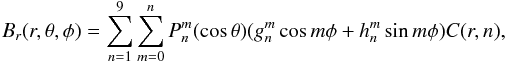 (1)where
  are the associated Legendre functions, r is the radial distance, θ is the colatitude (polar angle), and φ is the longitude. Here we neglect the nonphysical magnetic monopole term (m = n = 0) by starting from n = 1. An alternative method is to modify synoptic maps by subtracting the overall mean value to force the
  coefficient to be zero (Altschuler & Newkirk 1969), which leads to exactly the same results.
The radial functions C(r,n) in Eq. (1) are ![\begin{equation} C(r,n) = \left(\frac{R}{r}\right)^{n+2} \left[\frac{n+1+n\left(\frac{r}{r_{\rm ss}}\right)^{2n+1}}{n+1+n\left(\frac{R}{r_{\rm ss}}\right)^{2n+1}} \right], \label{eq:pfss2} \end{equation}](/articles/aa/full_html/2016/07/aa28096-16/aa28096-16-eq17.png) (2)where R is the solar radius. When the measured data is given in the longitude – sine-latitude grid, harmonic coefficients
(2)where R is the solar radius. When the measured data is given in the longitude – sine-latitude grid, harmonic coefficients  and
and  are as follows:
 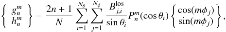 (3)where
  refers to the measured photospheric line-of-sight value at longitude – sine-latitude bin (j,i), and sin(θi)-1 term comes from the assumption that the photospheric magnetic field is radial, and N is the number of existing data points in the grid. In case of full data coverage N = NφNθ, where Nφ is the number of data bins in longitude and Nθ is the number of data bins in latitude. The solid angle covered by each cell is constant ΔΩ = 4π/NφNθ.
When the measured data is given in the longitude-latitude grid, the bin area (and solid angle) decreases with latitude and ΔΩ = sinθΔθΔφ, where Δθ = π/Nθ and Δφ = 2π/Nφ. In this case, the harmonic coefficients are as follows: 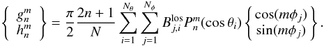 (4)In the case of KP, SOLIS, MDI, and HMI data the synoptic maps show the Br-component, i.e., the maps have been already scaled by the sin(θi)-1 term. Instead, the WSO and MWO synoptic maps give the line-of-sight component, so that Eq. (4) applies to MWO without modification. Irrespective of the accuracy of the original synoptic maps of the measured magnetic field, we always solve the coronal magnetic field from harmonic coefficients in the same Carrington grid of 72 points in longitude and 30 points in sine latitude, which is also the accuracy used in coronal maps published by WSO.
2.3. North-south shift of HCS
After calculating the coronal magnetic field at the source surface (rss = 2.5 R), we sum up all bins of the two magnetic polarities to find the total solid angles  (
( ) covered by positive (Br away from the sun) and negative (Br toward the sun) polarities. Following the method presented earlier (Zhao et al. 2005; Virtanen & Mursula 2014), we can solve the (longitudinally averaged) shift (displacement) of the HCS from the Sun’s magnetic dipole equator, i.e., the average heliomagnetic latitude of the heliospheric current sheet during one Carrington rotation in terms of the fractional solid angle covered by the positive polarity,
 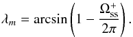 (5)If λm systematically deviates from zero during several rotations, the area of the corresponding polarity field is larger than the other.
However, the magnetic dipole equator and heliographic equator are not aligned in general. The tilt angle α between the solar rotation axis and magnetic dipole axis reaches its minimum during solar minimum and its maximum during solar maximum. The longitudinally averaged shift of the HCS from the heliographic equator, i.e., the average heliographic latitude of the heliospheric current sheet during one Carrington rotation is obtained as follows (Zhao et al. 2005; Virtanen & Mursula2014):  (6)There are several possible methods to define and calculate the tilt α. We use here the definition adopted at WSO, where α is the average of the maximum northern and maximum southern extension of the HCS, defined from the synoptic map of the coronal magnetic field for each rotation. The WSO tilt values are available from Carrington rotation 1642 onward. For the two previous years, we use MWO coronal maps and the same definition as at WSO to calculate the α values.
We study both λm and λh shifts, since they give a complementary presentation of the coronal source surface field. The magnetic shift λm reveals the possible asymmetry between the two polarities, i.e., whether one polarity dominates over the other. On the other hand, the heliographic shift λh sets the HCS location in the polarity-independent heliographic reference frame, which is relevant, for example, when comparing the coronal asymmetry with observations in the heliosphere. Also, around solar maximum times the HCS is highly tilted and, therefore, the shifts λh tend to be close to zero even if λm were rather large.
The three dipole terms, the axial dipole term  , and the two equatorial dipole terms
  and
and  , are the most significant harmonics, for example, for the tilt and overall structure of the HMF during most of the solar cycle. On the other hand, the lowest north-south symmetric harmonic term, which is the axisymmetric (axial) quadrupole term
  , is known to be important for the hemispheric asymmetry of the coronal and heliospheric magnetic fields (Zhao et al. 2005; Virtanen & Mursula 2014).
3. Results
Figure 1 shows the so-called magnetic butterfly diagrams of the measured photospheric magnetic field, i.e., the longitudinal averages of rotational synoptic maps. The first impression from Fig. 1 is that the different data sets show a very similar large-scale structure. Poleward surges of magnetic flux appear mostly similarly in each panel, but active regions look somewhat different, mainly owing to the different spatial resolution between the six data sets. Improved spatial resolution makes more complicated, multipolar structures visible.
3.1. Photosphere: Polar fields and reversals
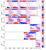 |
Fig. 1 Longitudinal averages of the synoptic maps of the photospheric magnetic field in latitude – time presentation for the six data sets. Color indicates the field intensity. |
Polar field reversals are observed around 1980, 1991, 2001, and 2014. Reversal timings vary slightly between the six data sets and the northern and southern reversals are typically not simultaneous. In the beginning of WSO, MWO, and KP observations after the mid-1970s, the polar fields have a typical minimum time configuration. Surprisingly, KP data show negative polarity even in the northern hemisphere during short intervals in 1975 and in 1976, but these results are most likely due to errors in KP data; Table 2 includes the periods of the main errors suggested by this study. Negative polarity in the north at KP at this time is in disagreement with the simultaneous observations carried out at WSO and MWO, and even with the positive polarity data taken at KP in several subsequent years. Polarity reversal in the north is observed rather simultaneously in 1980 in WSO and MWO data, but after a short period of negative polarity in that time period, KP results mostly show positive polarity until 1982, when it finally reverses to negative. In the southern hemisphere, the reversal is observed in 1981 with no major differences between the three data sets. The development of polar fields in the 1980s, during the declining phase of SC21 and the ascending phase of SC22, is similar in the WSO and MWO data, but the polar fields at KP depict some errors. The southern polar field in the KP data remains rather weak until this field experiences an artificial stepwise increase in 1985. On the other hand, the northern polar field in KP remains rather patchy and weak over the 1980s, in contradiction with the WSO and MWO observations.
Longest time intervals when a significant fraction of data are questionable based on the present study.
The reversal of polar fields during solar cycle 22 is observed again very similarly in the WSO and MWO data. WSO shows the reversal in the north in late 1990 and MWO only slightly later in early 1991. A very strong surge of negative polarity flux reverses the southern polar field in both the WSO and MWO data in 1991, however, the MWO data depict weak patches of the old polarity at the highest southern latitudes during the best visibility of the south pole in spring 1992. The KP results depict this reversal as proceeding very differently and, most likely, erroneously. The old negative polarity in the north is seen to be very strong until 1992 and, thereafter, the northern polar field reverses abruptly. In the southern hemisphere, the KP data indicate an early polar field reversal in 1990. Accordingly, in 1990–1992, the KP data have strong negative polarity fields at both poles, a unique monopole configuration, which conflicts with WSO and MWO observations and is almost certainly erroneous.
During the maximum time of SC23, MDI measurements of the photospheric magnetic field were also available from the SOHO satellite. The northern pole in the WSO results reverses at the turn of 2000–2001 and the southern pole only few months later. However, in the WSO data, the northern polar field reverses temporally in spring 2000 already. This early reversal may be due to the low resolution and vantage point effect. Also, the old positive polarity field was recovered when visibility of the north pole was optimum in fall 2000. The same oscillation is seen even more clearly in the southern hemisphere, where the WSO data set shows temporal polar field reversals in fall 1999 and 2000, when the viewing of high southern latitudes was difficult. Moreover, the WSO results depict extremely strong negative southern polar fields in spring 2001, during the best visibility of the south pole while, at the same time, the last remnants of negative polarity are seen to dominate in the south according to the higher resolution (and higher latitude) measurements of MWO, KP, and MDI. This verifies that the (multiple) earlier reversals in WSO are due to the low resolution and vantage point effect, while the polar field reversal of SC23 is seen to evolve very smoothly and rather similarly in MWO, KP, and MDI. The KP data set indicates reversal in the north in early 2001 already, while the MWO and MDI results show significant amount of positive polarity until mid-2001.
During the declining phase of SC23 and the subsequent minimum, the polar fields were much weaker than during the three previous minima (Smith & Balogh 2008; Wang et al. 2009), although this is not very visible in Fig. 1 due to finite color resolution. The reversal of polarity of SC24 is monitored by WSO, SOLIS, and HMI. The WSO data indicate a temporal reversal in the north in spring 2011 already and there is a short reversal in SOLIS in spring 2012; these reversals are both likely owing to the vantage point effect. The next reversal of the northern polar field is seen in the WSO data in late 2012 as a consequence of a strong poleward surge of positive polarity, which emerged as an active region in early 2011. A similar evolution is seen in SOLIS and HMI, where the dominance of negative polarity in the northern pole ended by the end of 2012. All three data sets show that the northern polar field remains rather weak until the end the of included interval (June 2015), and that a significant surge of old negative polarity still reached the northern pole in 2014, turning the polarity temporarily in WSO and SOLIS. The southern polar field reversal is first observed in the WSO results in summer 2013, but the polar field remains very small and even reverses back to positive in fall 2014, probably again because of the vantage point effect. The final reversal of the southern polar field in early 2015 is related to a strong surge of negative flux and evidenced very similarly by all three data sets. Overall, SOLIS and HMI depict a more systematic evolution of the southern polar field during SC24 than WSO. The strong surge of negative flux intensifies the southern polar field, making it, at least until the end of the time interval included, much stronger than the northern polar field.
Polar field reversals have been studied in detail, for example, by Petrie et al. (2014) and Sun et al. (2015), and in general the results based on different instruments and data set are in fairly good agreement. However, as we have discussed above, differences may occur, when the weak fields around the north (south) pole are observed in the unfavorable vantage point location in spring (fall), respectively. The coarse resolution of WSO gives more weight to the field at lower latitudes, hence, the polar field reversal in the WSO is typically seen several months before the old polarity actually disappears from the highest latitudes. Moreover, during reversals, the weak polar fields may be quite noisy. For example, in the MWO and HMI data sets we sometimes see pixels of wrong polarity at the highest latitudes during reversal times. We also note that the missing pixels of the poles (at certain times) have been filled in KP, SOLIS, and MDI when constructing the synoptic maps. Filling methods are also different. In MDI, the polar field filling method also effectively removes both the erroneous pixels and the annual oscillation due to the vantage point effect, leading to a very smooth reversal of SC23. As we already pointed out, polar fields in the KP data are erroneous especially in the 1980s. Petrie (2015) shows an improved version of the KP magnetic butterfly diagram, where obvious errors have been filtered out. Also, filtered polar field observations of SOLIS are available at NSO site7.
3.2. Coronal field
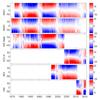 |
Fig. 2 Longitudinal averages of the synoptic maps of the coronal magnetic field for the six data sets, derived using synoptic maps of the photospheric magnetic field and the PFSS model. |
Figure 2 shows the coronal magnetic field at the source surface distance for the six data sets. One can see the fairly similar overall structure of the coronal field in all of the instruments over the depicted time interval. The mainly dipolar structure of the coronal field over most of the solar cycle, the approximate timing of polarity reversals, and the complex field structure during the solar maxima are very similarly depicted in all of the data sets.
However, there are also differences in Fig. 2 between the instruments that are, naturally, related to the above discussed differences in the photospheric field. For example, the annual variation of the heliospheric current sheet (the white area between the two opposite polarities) is markedly strong in the MWO data set. This is, as explained above, due to the vantage point effect, and the fact that the in MWO data, no filling of polar fields is made. Rather, the observations in the two hemispheres extend typically to different latitudes and the latitude ranges covered in either hemisphere alternate systematically during the year. This is seen clearly in Fig. 1.
The annual variation of the heliospheric current sheet due to the vantage point effect is also very strong and systematic in the WSO data set where, due to the low spatial resolution, the effective latitude of observations experiences a strong annual variation. The annual variation of the HCS can also be seen at times in the KP and SOLIS data, but much more weakly and less systematically than in the MWO and WSO data sets. Moreover, this effect is practically absent in the MDI and HMI data sets, most likely due to careful filling of polar fields and higher spatial accuracy, respectively.
Most of the differences in the photospheric field between the instruments, some due to errors in some instrument, as discussed above, are also seen in the coronal field of Fig. 2, sometimes even standing out more clearly there than in the photosphere. For example, the problems with the KP data set in the late 1970s, as well as around the polarity reversals of cycles 21 and 22, are very clearly seen in Fig. 2. Also, the artificial, abrupt intensification of the southern photospheric field in 1985 in the KP data set is seen as a sudden decrease of the latitudinal extent of the HCS at this time in Fig. 2. On the other hand, the multiple reversal of the southern photospheric field seen in the WSO data set during the maximum of SC23 is less clearly reproduced in the coronal field in Fig. 2 than in the photosphere.
The weaker photospheric magnetic field during SC23 and SC24 is also clearly seen in the weaker coronal field at these times, especially in the WSO and MWO data sets, which allow for a long-term monitoring of the coronal field. In addition, the annual variation of the heliospheric current sheet in the WSO and MWO data sets is slightly stronger during these times as a result of the weaker coronal field and the wider extent of the HCS during most of the declining phase of SC23.
3.3. Shift of the heliospheric current sheet
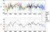 |
Fig. 3 Heliomagnetic shift λm of the HCS in the solar corona, derived for the six data sets using their measurements of the photospheric field and the PFSS model. Upper panel shows the Carrington rotational values and the lower panel the 13-rotation running means. |
Figure 3 shows the heliomagnetic HCS shift λm derived from Eq. (5) for all six data sets. The upper panel shows the rotational values where the annual oscillation due to the vantage point effect is clearly visible, especially in the MWO data set. The lower panel depicts the λm values smoothed over 13 rotations (in steps of one rotation), where the annual variation is mostly removed. We have requested that 7 out of 13 rotations must have a measured λm for each smoothed value. Unless otherwise mentioned, when referring to λm, we always mean the 13-rotation smoothed values. The agreement between smoothed λm values from the different data sets is at least reasonable. From 1975 to 1979, the MWO, WSO, and KP data all depict a dominance of negative λm. Accordingly, the HCS was mainly shifted toward the southern magnetic hemisphere at this time, suggesting that the bashful ballerina phenomenon occurred in the late declining to minimum phase of SC20. This can be verified by the observations of the heliospheric magnetic field at 1 AU; see Mursula & Hiltula (2003). The amount of shift is largest in the MWO data from 1975–1976. As noted above (see also Table 2), the KP data are erroneous in the 1970s. The same polarity dominates both poles in the KP data (see Fig. 1) from 1976–1977, leading to the excessively negative value of λm at this time (see Fig. 3). In 1979–1982, the KP data depict slightly higher values of λm than data sets from the other two instruments; this is most likely related to the problematic evolution of northern polar fields at this time (see Fig. 1).
From 1983 to 1987 there is a period when the HCS is systematically shifted toward the northern magnetic hemisphere according to all three instruments. This is the bashful ballerina period of SC21. Kitt Peak shows excessively large positive λm in 1985–1989, which is related to the erroneously large intensity of the southern polar field at this time (see Fig. 1 and Table 2). In 1988–1991, the ascending phase and maximum of SC22, λm (of WSO and MWO) remains rather small, oscillating around zero.
In the declining to minimum phase of SC22, in 1991–1997, λm is continuously and very strongly negative according to all three ground-based data sets. The WSO data set deviates from the other two in 1996–1999 because of the error noted above; see also Table 2. The MDI results agreed with this from 1996–1997. This is the bashful ballerina period of SC22. At this time, the negative polarity field of the southern pole is systematically stronger than the positive field of the north pole. The λm shift of about 5° in 1993–1994 is so large that almost all of the rotational λm values of all of the data sets, in part even the MWO data, are negative, thus overwhelming the vantage point effect and confirming its insignificant role for the shift. During the maximum years in 1999–2000 the rotational values of λm oscillate strongly, but the smoothed values remain close to zero. The problems in WSO culminate in 2001, when the highest rotational λm value of all time in any data set of about –21.5° is obtained for the erroneous WSO data (see Table 2).
In 2001–2003 and again in 2007–2009 λm is positive, indicating the bashful ballerina period of solar cycle 23. However, the shift λm is smaller and less systematic (interrupted by weakly negative asymmetry in 2005–2006) than during cycles 21 and 22. Despite the lower value and the more complex evolution of λm, all data sets agree on two periods of positive λm, intervened by a negative λm period. This provides additional support for the earlier results of the southward HCS shift in SC23, obtained using both ground-based (Mursula & Virtanen 2011) and satellite observations (Virtanen & Mursula 2010; Erdös & Balogh 2010). The weak polar fields of SC23 (Smith & Balogh 2008; Wang et al. 2009), leading to a wider HCS for most of this time, make the observations of the HCS shift more difficult (Mursula & Virtanen 2011). However, Ulysses observations show (Virtanen & Mursula 2010; Erdös & Balogh 2010) that the HCS shift was the same, about 2°, during SC23 (the fast latitude scan in 2007) as during SC22 (in 1994/1995), when polar fields were considerably stronger.
The evolution of λm during SC24 is not yet fully concluded since the data only extends until summer 2015, one year after sunspot maximum. Still, the three instruments that continue their operation until today (WSO, SOLIS and HMI) depict a very similar evolution of λm since 2010, favoring negative values during the recent times of the early declining phase of SC24.
After the dipole reversal in 2014, the negative λm corresponds to the southward shifted HCS, in agreement with several earlier cycles. So, this may be the start of the bashful ballerina period of SC24. Simultaneously, all three data sets indicate a rapid strengthening of the negative southern polar field (see Figs. 1 and 2), leading to the negative λm. During the last two years | λm | is few degrees larger in the WSO than in HMI or SOLIS data sets, evidently because of the more coarse spatial resolution of WSO data, which has the highest bin at lower latitude (and stronger field) than in the other data sets. Accordingly, although some caveat still remains, the three data sets show a consistently negative λm in the rather early declining phase of SC24, similar to SC22.
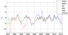 |
Fig. 4 Heliographic shift λh of the HCS in the solar corona (13-rotation running means) derived for the six data using their measurements of the photospheric field and the PFSS model. |
Figure 4 depicts the 13-rotation running means of λh, the heliographic shift of the HCS, derived from Eq. (6). Because of the cosα-term, the HCS shift in the heliographic coordinate system is significantly smaller than λm during solar maximum times. This is particularly true around 1980 (compare Figs. 3 and 4). The λh gives the mean HCS asymmetry in the heliosphere and determines the long-term effect that the Earth’s magnetosphere experiences as a result of a non-zero HCS asymmetry. As seen in Eq. (6), λh is oriented oppositely due to λm for periods of negative α (negative solar polarity). Therefore, while positive (negative) λm corresponds to the HCS shifted parallel (antiparallel) to the (possibly tilted) dipole, positive (negative) λh means that the HCS is shifted above (below) the solar equator. Figure 4 shows that the HCS is shifted below the solar equator, i.e., toward the southern heliographic hemisphere during the declining to minimum phase of all the three fully covered SC21, SC22, and SC23. There is also strong evidence of a southward shift during SC20 and SC24. Thus, the phenomenon of the bashful ballerina (Mursula & Hiltula 2003) is consistently valid since 1974 according to six magnetographs in agreement with results based on heliospheric observations (Mursula & Virtanen 2012) and heliospheric-solar comparison (Mursula & Virtanen 2011).
3.4. Effect of the quadrupole term
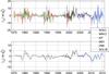 |
Fig. 5 Heliomagnetic shift λm(no |
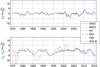 |
Fig. 6 Upper panel: 13-rotation running means of the heliographic shift λh(no |
We have tested the effect of the axial quadrupole term ( term in Eq. (1)) on the HCS shift. This is the lowest hemispherically symmetric term and its importance on the north-south asymmetry was in earlier publications (Mursula & Hiltula 2004; Zhao et al. 2005; Wang & Robbrecht 2011; Virtanen & Mursula 2014). Figure 5 shows the values of the “no-quadrupole” heliomagnetic shift λm(no ), where the term was removed from the harmonic expansion of Eq. (1) before calculating the coronal magnetic field and the shift λm. Comparing the lower panels of Figs. 3 and 5 shows that the shift |λm(no )| is consistently smaller than |λm| in late 1970s, 1980s, and 1990s, i.e., during the declining to minimum phases of SC20, SC21, and SC22. However, removing the quadrupole term has no such effect during SC23. In fact, the positive values of λm(no ) in the early 2000s are higher than in λm, and the negative values in 2005–2006 disappear from λm(no ). Accordingly, it is clear that the HCS shift during cycle 23 is not due to the quadrupole term, unlike all of the earlier cycles. Figure 5 also shows that the southward shift of the HCS in 2014–2015 is again at least mainly due to the quadrupole term, while the higher harmonics tend to produce an alternating λm(no ) with a weak northward shift in 2014–2015.
The differences in λm(no ) values between the six data sets are much smaller than in λm (compare the lower panels of Figs. 3 and 5). Also, the annual oscillation due to the vantage point effect is much smaller in the rotational values of λm(no ) than in λm. This is most dramatically seen in the MWO data set, where the annual oscillation almost disappears in λm(no ).
Figure 6 depicts the 13-rotation running mean values of the heliographic shift λh(no ) calculated from the heliomagnetic shift λm(no ) and the difference between λh and the λh(no ). It is clearly seen in Fig. 6 that the quadrupole term is mainly responsible for the southward shift of the HCS during solar cycles 20–22 and 24, but not during cycle 23. These results verify the earlier observations that the hemispheric asymmetry and the HCS shift during SC20 – 22 are mainly due to the quadrupole harmonic term (Zhao et al. 2005; Virtanen & Mursula 2014).
We showed earlier (Virtanen & Mursula 2014) that the term already starts developing during the ascending phase, when new flux is transported to the poles, reaching its maximum value (the bashful ballerina period) in the declining phase when the polar latitudes are mainly responsible for the term and HCS asymmetry. The present results show that the term is mainly responsible for the vantage point effect and for the mutual differences in the coronal field between the different data sets. They therefore emphasize the need for correctly observing and treating the measurements at the highest solar latitudes, especially in the declining to minimum phase of the solar cycle. Despite occasional problems in most data sets, they mainly agree with each other and, thereby, allow us to construct a reliable picture of the coronal magnetic field and its hemispheric asymmetry.
4. Discussion
We studied the long-term evolution of the solar photospheric and coronal magnetic fields and the hemispheric asymmetry of the heliospheric current sheet using data from six different instruments: WSO, MWO, KP, SOLIS, MDI, and HMI. We showed that, despite several differences in measurement techniques and data treatment practices (e.g., filling of polar latitudes, forming of the synoptic maps) and occasional errors in some instruments, all of the data sets give a consistent view of the evolution of the heliospheric current sheet and, in particular, on its southward shift in the declining to minimum phase of the solar cycle (the bashful ballerina phenomenon). All of the instruments agree that the HCS was southward shifted during several (typically three) years in the declining to minimum phase of cycles 20–23. Even now, in the early declining phase of solar cycle 24, we find the HCS to be southward shifted, soon after polarity reversal in 2014. However, it is still premature to say whether this will be the dominant pattern for the declining to minimum phase of cycle 24.
The agreement is notable for two of the longest-running data sets, WSO and MWO, which indicate a closely similar pattern of the southward shifted HCS in the 1970s, 1980s, 1990s, and 2000s. However, the KP results deviated from the WSO and MWO results for many years until the KP instrument was updated in 1992, whereafter the three data sets closely agree. There is also a persistent problem in WSO, which leads to a different evolution of the coronal field and HCS asymmetry in 1996–1999 and 2001 (The first problematic interval is due to an unknown, the second due to a known instrumental defect; T. Hoeksema, priv. comm.). At all times at least three instruments were operative. The best coverage was available during solar cycle 23, when four different instruments were available, with WSO, MWO, and KP (continued by SOLIS in 2003) on ground and MDI starting satellite observations in 1996.
Previously, Zhao et al. (2005) and Virtanen & Mursula (2014) showed, using WSO observations, that the southward shift of the HCS is, at least for solar cycles 21–22, due to the axial quadrupole term of the harmonic expansion of the photospheric magnetic field. In this paper, using the six magnetographs, we verify that the term causes the southward shift of the HCS during solar cycles 20–22, and 24. However, we find that during SC23 the HCS asymmetry is not caused by the axial quadrupole term, but by higher harmonics. Although the reasons for this difference are not yet fully understood, it is likely that they are related to the other changes in solar magnetic fields during the declining phase of SC23, including the weak polar fields (Smith & Balogh 2008; Wang et al. 2009) and the changes in the properties of sunspots and their mutual relations with several other solar parameters (Lukianova & Mursula 2011; Lefèvre & Clette 2011; Tapping & Valdés 2011).
The observed differences between the six data sets can be mostly traced to known instrument problems. Some differences relate to the measurement and treatment of polar fields, which are the main contributor to the -term. Polar field measurements suffer from poor and variable visibility and the annual oscillation due to the Earth’s varying heliographic latitude, the so-called vantage point effect. The size of the vantage point effect varies between the data sets because it is most systematic at the MWO (see, e.g., Figs. 1 and 3). However, as we have shown in this paper (see, e.g., Figs. 4 and 6), the large-scale structure of the coronal field and the HCS shift are not produced or masked by the vantage point effect , and neither are they produced by the differences in observation nor by the polar field treatment.
Solar polar magnetic fields are a key parameter in solar activity studies and, via their effect on the solar wind, play a crucial role in solar-terrestrial physics. Several parameters of solar activity are north-south asymmetric, including the sunspots, which tend to appear preferably in the north before the maximum and in the south after the maximum, at least during the most recent cycles (Temmer et al. 2006). Similarly, polar fields and polar coronal holes are formed with some delay and difference in the two hemispheres (Mursula & Virtanen 2012). As we showed earlier (Virtanen & Mursula 2014), polar fields are formed asymmetrically by poleward surges of magnetic flux, which are generated and transported differently in the northern and southern hemispheres. The origin of the asymmetric evolution of these surges is not known in detail. Some studies, simulating the flux transport, show that the asymmetry can arise purely from an asymmetric generation of active regions (Wang & Robbrecht 2011), but it also may relate to the north-south asymmetric meridional flow (Rightmire-Upton et al. 2012). We also noted earlier that the polar fields typically reverse earlier in the northern hemisphere, while in the beginning of the cycle in the south, there are typically more surges of opposite polarity (Virtanen & Mursula 2014). The total amount of flux transported to the southern pole is larger than to the north, eventually making the magnetic flux density larger in the southern hemisphere during the minimum.
5. Conclusions
Synoptic measurements of the photospheric magnetic field since the 1970s offer an excellent data base for space climate studies. We have shown that despite some differences and errors the measurements by six different instruments give a coherent overall view of the evolution solar magnetic fields and the heliospheric current sheet over four decades. However, there are a few periods when one instrument disagrees with the others. KP measurements significantly deviate from the two others (WSO and MWO) for many years until the instrument update in 1992; WSO measurements deviate from the others (MWO and KP) in 1996–1999 and 2001. We are confident that the synoptic maps of these instruments at these times are erroneous; the MWO data are somewhat questionable in 2010–2012. The six data sets verify the southward shift of the heliospheric current sheet typically during three years in the declining to minimum phase of the cycle (the bashful ballerina phenomenon) for all of the studied solar cycles 20–24 (cycle 24 still preliminary).
We showed here that the southward HCS shift is for cycles 20–22 and, most likely also for cycle 24, mainly due to the axial quadrupole term of the harmonic expansion of the photospheric magnetic field. On the other hand, during cycle 23 the asymmetry is related to higher harmonics. This makes cycle 23 unique in the hemispheric asymmetry among the other five solar cycles. We note that cycle 23 depicts unique features that are also related to sunspots and their relation of other forms of solar activity; see, e.g., Lukianova & Mursula (2011), Lefèvre & Clette (2011), Tapping & Valdés (2011). The term reflects the larger magnetic flux density of the southern polar field during the bashful ballerina times and is formed by north-south asymmetric surges of magnetic flux, generated at midlatitudes during solar maximum times and drifting poleward. The hemispheric asymmetry of polar fields may results from the north-south asymmetric generation, the evolution of active regions, or from an asymmetric meridional transport. The fundamental question is what mechanisms in the solar dynamo can cause and sustain such hemispheric asymmetries.
Acknowledgments
We acknowledge the financial support by the Academy of Finland to the ReSoLVE Centre of Excellence (project No. 272157). Wilcox Solar Observatory data used in this study were obtained via the web site http://wso.stanford.edu courtesy of J.T. Hoeksema. This study includes data from the synoptic program at the 150-Foot Solar Tower of the Mt. Wilson Observatory. The Mt. Wilson 150-Foot Solar Tower is operated by UCLA with funding from NASA, ONR, and NSF, under agreement with the Mt. Wilson Institute. NSO/Kitt Peak magnetic data used here are produced cooperatively by NSF/NOAO, NASA/GSFC, and NOAA/SEL. Data were acquired by SOLIS instruments operated by NISP/NSO/AURA/NSF. SOHO/MDI is a project of international cooperation between ESA and NASA. HMI data are courtesy of the Joint Science Operations Center (JSOC) Science Data Processing team at Stanford University. We also acknowledge Roger Ulrich, Jack Harvey, and Luca Bertello for maintaining the data bases and help in their availability. The authors thank the anonymous referee for the constructive comments that improved this article.
References
- Altschuler, M. D., & Newkirk, G. 1969, Sol. Phys., 9, 131 [Google Scholar]
- Bertello, L., Pevtsov, A. A., Petrie, G. J. D., & Keys, D. 2014, Sol. Phys., 289, 2419 [Google Scholar]
- Crooker, N. U., Lazarus, A. J., Phillips, J. L., et al. 1997, J. Geophys. Res., 102, 4673 [NASA ADS] [CrossRef] [Google Scholar]
- Erdös, G., & Balogh, A. 2010, J. Geophys. Res. (Space Phys.), 115, 1105 [Google Scholar]
- Harvey, J. 2000, ftp://vso.nso.edu/kpvt/synoptic [Google Scholar]
- Harvey, J., & Munoz-Jaramillo, A. 2015, in AAS/AGU Triennial Earth-Sun Summit, Vol. 1, http://nisp.nso.edu/sites/nisp.nso.edu/files/images/poster/spd2015/jh.pdf, 11102 [Google Scholar]
- Hiltula, T., & Mursula, K. 2006, Geophys. Res. Lett., 33, L03105 [NASA ADS] [CrossRef] [Google Scholar]
- Hoeksema, J. T., Wilcox, J. M., & Scherrer, P. H. 1983, J. Geophys. Res., 88, 9910 [NASA ADS] [CrossRef] [Google Scholar]
- Käpylä, M. J., Käpylä, P. J., Olspert, N., et al. 2016, A&A, 589, A56 [NASA ADS] [CrossRef] [EDP Sciences] [Google Scholar]
- Lefèvre, L., & Clette, F. 2011, A&A, 536, L11 [NASA ADS] [CrossRef] [EDP Sciences] [Google Scholar]
- Lukianova, R., & Mursula, K. 2011, J. Atm. Solar-Terrestrial Phys., 73, 235 [NASA ADS] [CrossRef] [Google Scholar]
- McIntosh, S. W., Leamon, R. J., Gurman, J. B., et al. 2013, ApJ, 765, 146 [NASA ADS] [CrossRef] [Google Scholar]
- Mursula, K., & Hiltula, T. 2003, Geophys. Res. Lett., 30, 2135 [Google Scholar]
- Mursula, K., & Hiltula, T. 2004, Sol. Phys., 224, 133 [Google Scholar]
- Mursula, K., & Virtanen, I. I. 2011, A&A, 525, L12 [NASA ADS] [CrossRef] [EDP Sciences] [Google Scholar]
- Mursula, K., & Virtanen, I. I. 2012, J. Geophys. Res. (Space Phys.), 117, 8104 [NASA ADS] [CrossRef] [Google Scholar]
- Mursula, K., & Zieger, B. 2001, Geophys. Res. Lett., 28, 95 [NASA ADS] [CrossRef] [Google Scholar]
- Mursula, K., Hiltula, T., & Zieger, B. 2002, Geophys. Res. Lett., 29, 1738 [Google Scholar]
- Norton, A. A., & Gallagher, J. C. 2010, Sol. Phys., 261, 193 [NASA ADS] [CrossRef] [Google Scholar]
- Norton, A. A., Charbonneau, P., & Passos, D. 2014, Space Sci. Rev., 186, 251 [NASA ADS] [CrossRef] [Google Scholar]
- Petrie, G. J. D. 2015, Liv. Rev. Sol. Phys., 12 [Google Scholar]
- Petrie, G. J. D., & Patrikeeva, I. 2009, ApJ, 699, 871 [NASA ADS] [CrossRef] [Google Scholar]
- Petrie, G. J. D., Petrovay, K., & Schatten, K. 2014, Space Sci. Rev., 186, 325 [NASA ADS] [CrossRef] [Google Scholar]
- Richardson, J. D., & Paularena, K. I. 1997, Geophys. Res. Lett., 24, 1435 [NASA ADS] [CrossRef] [Google Scholar]
- Rightmire-Upton, L., Hathaway, D. H., & Kosak, K. 2012, ApJ, 761, L14 [Google Scholar]
- Riley, P., Ben-Nun, M., Linker, J. A., et al. 2014, Sol. Phys., 289, 769 [Google Scholar]
- Schatten, K. H., Wilcox, J. M., & Ness, N. F. 1969, Sol. Phys., 6, 442 [Google Scholar]
- Smith, E. J., & Balogh, A. 2008, Geophys. Res. Lett., 35, 22103 [NASA ADS] [CrossRef] [Google Scholar]
- Smith, E. J., Balogh, A., Forsyth, R. J., & McComas, D. J. 2001, Geophys. Res. Lett., 28, 4159 [NASA ADS] [CrossRef] [Google Scholar]
- Sun, X. 2009, http://wso.stanford.edu/words/pfss.pdf [Google Scholar]
- Sun, X., Liu, Y., Hoeksema, J. T., Hayashi, K., & Zhao, X. 2011, Sol. Phys., 270, 9 [NASA ADS] [CrossRef] [Google Scholar]
- Sun, X., Hoeksema, J. T., Liu, Y., & Zhao, J. 2015, ApJ, 798, 114 [NASA ADS] [CrossRef] [Google Scholar]
- Svalgaard, L., & Kamide, Y. 2013, ApJ, 763, 23 [NASA ADS] [CrossRef] [Google Scholar]
- Svalgaard, L., Duvall, Jr., T. L., & Scherrer, P. H. 1978, Sol. Phys., 58, 225 [Google Scholar]
- Tapping, K. F., & Valdés, J. J. 2011, Sol. Phys., 272, 337 [NASA ADS] [CrossRef] [Google Scholar]
- Temmer, M., Rybák, J., Bendík, P., et al. 2006, A&A, 447, 735 [NASA ADS] [CrossRef] [EDP Sciences] [Google Scholar]
- Ulrich, R. K., & Tran, T. 2013, ApJ, 768, 189 [NASA ADS] [CrossRef] [Google Scholar]
- Upton, L., & Hathaway, D. H. 2014, ApJ, 780, 5 [NASA ADS] [CrossRef] [Google Scholar]
- Vernova, E. S., Mursula, K., Tyasto, M. I., & Baranov, D. G. 2002, Sol. Phys., 205, 371 [NASA ADS] [CrossRef] [Google Scholar]
- Virtanen, I. I., & Mursula, K. 2010, J. Geophys. Res. (Space Phys.), 115, 9110 [Google Scholar]
- Virtanen, I. I., & Mursula, K. 2014, ApJ, 781, 99 [Google Scholar]
- Wang, Y.-M., & Robbrecht, E. 2011, ApJ, 736, 136 [NASA ADS] [CrossRef] [Google Scholar]
- Wang, Y.-M., & Sheeley, Jr., N. R. 1988, J. Geophys. Res., 93, 11227 [NASA ADS] [CrossRef] [Google Scholar]
- Wang, Y.-M., & Sheeley, Jr., N. R. 1992, ApJ, 392, 310 [NASA ADS] [CrossRef] [Google Scholar]
- Wang, Y.-M., Robbrecht, E., & Sheeley, Jr., N. R. 2009, ApJ, 707, 1372 [NASA ADS] [CrossRef] [Google Scholar]
- Zhang, J., & Feng, W. 2015, AJ, 150, 74 [NASA ADS] [CrossRef] [Google Scholar]
- Zhao, X. P., Hoeksema, J. T., & Scherrer, P. H. 2005, J. Geophys. Res., 110, 10101 [Google Scholar]
- Zieger, B., & Mursula, K. 1998, Geophys. Res. Lett., 25, 841 [NASA ADS] [CrossRef] [Google Scholar]
All Tables
Longest time intervals when a significant fraction of data are questionable based on the present study.
All Figures
|
Fig. 1 Longitudinal averages of the synoptic maps of the photospheric magnetic field in latitude – time presentation for the six data sets. Color indicates the field intensity. |
| In the text | |
|
Fig. 2 Longitudinal averages of the synoptic maps of the coronal magnetic field for the six data sets, derived using synoptic maps of the photospheric magnetic field and the PFSS model. |
| In the text | |
|
Fig. 3 Heliomagnetic shift λm of the HCS in the solar corona, derived for the six data sets using their measurements of the photospheric field and the PFSS model. Upper panel shows the Carrington rotational values and the lower panel the 13-rotation running means. |
| In the text | |
|
Fig. 4 Heliographic shift λh of the HCS in the solar corona (13-rotation running means) derived for the six data using their measurements of the photospheric field and the PFSS model. |
| In the text | |
|
Fig. 5 Heliomagnetic shift λm(no |
| In the text | |
|
Fig. 6 Upper panel: 13-rotation running means of the heliographic shift λh(no |
| In the text | |
Current usage metrics show cumulative count of Article Views (full-text article views including HTML views, PDF and ePub downloads, according to the available data) and Abstracts Views on Vision4Press platform.
Data correspond to usage on the plateform after 2015. The current usage metrics is available 48-96 hours after online publication and is updated daily on week days.
Initial download of the metrics may take a while.