| Issue |
A&A
Volume 591, July 2016
|
|
|---|---|---|
| Article Number | A76 | |
| Number of page(s) | 7 | |
| Section | Astrophysical processes | |
| DOI | https://doi.org/10.1051/0004-6361/201527964 | |
| Published online | 20 June 2016 | |
Super-orbital variability of LS I +61°303 at TeV energies
1
ETH Zurich, 8093
Zurich,
Switzerland
2
Università di Udine, and INFN Trieste,
33100
Udine,
Italy
3
INAF National Institute for Astrophysics,
00136
Rome,
Italy
4
Università di Siena, and INFN Pisa, 53100
Siena,
Italy
5
Croatian MAGIC Consortium, Rudjer Boskovic Institute, University
of Rijeka, University of Split and University of Zagreb,
Croatia
6
Saha Institute of Nuclear Physics, 1/AF Bidhannagar, Salt Lake, Sector-1,
700064
Kolkata,
India
7
Max-Planck-Institut für Physik, 80805
München,
Germany
8
Universidad Complutense, 28040
Madrid,
Spain
9
Inst. de Astrofísica de Canarias, 38200
La Laguna, Tenerife,
Spain
10
Universidad de La Laguna, Dpto. Astrofísica, 38206
La Laguna, Tenerife,
Spain
11
University of Łódź, 90236
Lodz,
Poland
12
Deutsches Elektronen-Synchrotron (DESY),
15738
Zeuthen,
Germany
13
Institut de Fisica d’Altes Energies, The Barcelona Institute of
Science and Technology (IFAE-BIST), Campus UAB, 08193
Bellaterra ( Barcelona), Spain
14
Universität Würzburg, 97074
Würzburg,
Germany
15
Università di Padova and INFN, 35131
Padova,
Italy
16
Institute for Space Sciences (CSIC/IEEC),
08193
Barcelona,
Spain
17
Centro de Investigaciones Energéticas, Medioambientales y
Tecnológicas, 28040
Madrid,
Spain
18
Technische Universität Dortmund, 44221
Dortmund,
Germany
19
Unitat de Física de les Radiacions, Departament de Física, and
CERES-IEEC, Universitat Autònoma de Barcelona, 08193
Bellaterra,
Spain
20
Universitat de Barcelona, ICC, IEEC-UB,
08028
Barcelona,
Spain
21
Japanese MAGIC Consortium, ICRR, The University of Tokyo,
Department of Physics and Hakubi Center, Kyoto University, Tokai University, The
University of Tokushima, KEK, Japan
22
Finnish MAGIC Consortium, Tuorla Observatory, University of Turku
and Department of Physics, University of Oulu,
Finland
23
Inst. for Nucl. Research and Nucl. Energy,
1784
Sofia,
Bulgaria
24
Università di Pisa, and INFN Pisa, 56126
Pisa,
Italy
25
ICREA and Institute for Space Sciences (CSIC/IEEC),
08193
Barcelona,
Spain
26
Centro Brasileiro de Pesquisas Físicas (CBPF/MCTI),
R. Dr. Xavier Sigaud, 150 - Urca,
22290-180
Rio de Janeiro –
RJ,
Brazil
27
NASA Goddard Space Flight Center, Greenbelt, MD 20771, USA and
Department of Physics and Department of Astronomy, University of
Maryland, College
Park, MD
20742,
USA
28
Humboldt University of Berlin, Institut für Physik,
Newtonstr. 15, 12489
Berlin Germany
29
École polytechnique fédérale de Lausanne (EPFL),
Lausanne,
Switzerland
30
Department of Physics & Astronomy,
UC Riverside, CA
92521,
USA
31 Japanese MAGIC Consortium, Japan
32
Finnish Centre for Astronomy with ESO (FINCA),
Turku,
Finland
33 INAF-Trieste, Italy
34
ISDC – Science Data Center for Astrophysics,
1290 Versoix ( Geneva),
Switzerland
35
Laboratoire AIM, Service d’Astrophysique, DSM\IRFU,
CEA\Saclay, 91191
Gif-sur-Yvette Cedex,
France
Received: 15 December 2015
Accepted: 21 March 2016
Context. The gamma-ray binary LS I +61°303 is a well-established source from centimeter radio up to very high energy (VHE; E> 100 GeV). The broadband emission shows a periodicity of ~26.5 days, coincident with the orbital period. A longer (super-orbital) period of 1667 ± 8 days was proposed from radio variability and confirmed using optical and high-energy (HE; E> 100 MeV) gamma-ray observations. In this paper, we report on a four-year campaign performed by MAGIC together with archival data concentrating on a search for a long-timescale signature in the VHE emission from LS I +61°303.
Aims. We focus on the search for super-orbital modulation of the VHE emission, similar to that observed at other energies, and on the search for correlations between TeV emission and an optical determination of the extension of the circumstellar disk.
Methods. A four-year campaign has been carried out using the MAGIC telescopes. The source was observed during the orbital phases when the periodic VHE outbursts have occurred (φ = 0.55–0.75, one orbit = 26.496 days). Additionally, we included archival MAGIC observations and data published by the VERITAS collaboration in these studies. For the correlation studies, LS I +61°303 has also been observed during the orbital phases where sporadic VHE emission had been detected in the past (φ = 0.75–1.0). These MAGIC observations were simultaneous with optical spectroscopy from the LIVERPOOL telescope.
Results. The TeV flux of the periodical outburst in orbital phases φ = 0.5–0.75 was found to show yearly variability consistent with the long-term modulation of ~4.5 years found in the radio band. This modulation of the TeV flux can be well described by a sine function with a best-fit period of 1610 ± 58 days. The complete data, including archival observations, span two super-orbital periods. There is no evidence for a correlation between the TeV emission and the mass-loss rate of the Be star, but this may be affected by the strong, short-timescale (as short as intra-day) variation displayed by the Hα fluxes.
Key words: astroparticle physics / binaries: general / gamma rays: general / stars: individual: LS I +61°303 / X-rays: binaries / X-rays: individuals: LS I +61°303
© ESO, 2016
1. Introduction
LS I +61°303 (=V615 Cas ) is a gamma-ray binary composed of a rapidly rotating Be star of spectral type B0Ve (Hutchings & Crampton 1981) with a circumstellar disk and a compact object of unknown nature. The compact object, either a neutron star (NS) or a stellar-mass black hole (BH), has an eccentric orbit (e = 0.54 ± 0.03) with a period of 26.4960(28) days, determined from radio observations (Gregory 2002). The periastron passage occurs at phase φ = 0.23 ± 0.03, although its precise timing depends on the orbital solution (Gregory 2002; Casares et al. 2005; Grundstrom et al. 2007; Aragona et al. 2009)1.
LS I +61°303 is one of the few binary systems detected from radio to very high energy (VHE) gamma rays. The origin of the broadband emission is still under debate. LS I +61°303 was proposed as a microquasar, based on its extended jet-like radio-emitting structures, see Massi et al. (2004), for instance, and more recently, Massi & Torricelli-Ciamponi (2014). However, images obtained with the VLBA during a complete orbital cycle showed a rotating tail-like morphology of overall size 5–10 mas (Dhawan et al. 2006), consistent with a pulsar wind scenario (Maraschi & Treves 1981). Similar phase-resolved structures were later observed by Albert et al. (2008d). The source appears extended in X-rays (Paredes et al. 2007; Kargaltsev et al. 2014). Deep observations searching for X-ray pulsing have yielded only upper limits (Rea et al. 2010).
LS I +61°303 was first detected in the regime by MAGIC in 2006 (Albert et al. 2006). During the following years, moreobservations have been performed by the MAGIC (Albert et al. 2008d, 2009; Anderhub et al. 2009; Aleksić et al. 2012a) and VERITAS collaborations (Acciari et al. 2008). The VHE emission region is unresolved (<0.1deg). The system is also a HE gamma-ray Fermi/LAT source (Abdo et al. 2009). Long-term monitoring shows that the HE emission undergoes periodic outbursts slightly after the periastron passage, around phases φ~ 0.3–0.45 (Hadasch et al. 2012). In the orbit from MJD 53 752.7 until MJD 53 779.2 (January–February 2006), a TeV peak was first detected at phases φ~ 0.6–0.7 (which correspond to the phases next to the apastron) at a level of ~16% of the Crab Nebula flux for energies above 400 GeV. However, in October 2009–January 2010, the source was in a low flux state (Aleksić et al. 2012a) and the emission peak was above 300 GeV with a flux of only 5.4% of the Crab Nebula. Despite the state of the system, the highest TeV flux also occurred at phases φ = 0.6–0.7, consistent with previous observations. The spectral fit parameters agreed with our previous determinations (Albert et al. 2008d, 2009; Anderhub et al. 2009). Significant emission has also occasionally been observed at phases φ = 0.8–1, where MAGIC detected the system at ~4% Crab Units (C.U.) (Albert et al. 2009). Emission around periastron has been reported once, by VERITAS, in late 2010 at phase φ = 0.081 (Acciari et al. 2011) when the compact star was near superior conjunction.
Orbit-to-orbit variability has been associated with a super-orbital modulation. This was first proposed based on centimeter radio variations that show approximately sinusoidal modulation over 1667 ± 8 days (Paredes 1987; Gregory 2002). A similar long-term behavior has recently been suggested for X-rays (3–30 keV observed with RXTE; Li et al. 2012; Chernyakova et al. 2012), hard X-rays (18–60 keV observed with INTEGRAL; Li et al. 2014) and HE gamma-rays (100 MeV–300 GeV observed with Fermi/LAT; Ackermann et al. 2013). In the LAT energy range, the super-orbital variability is almost invisible around the periastron, where the compact object is inside (or highly affected by) the Be circumstellar disk, but appears around apastron.
Two short (<0.1 s) and very luminous (>1037 erg s-1) bursts have been detected from the direction of LS I +61°303 by the Swift Burst Alert Telescope (Barthelmy et al. 2008; Burrows et al. 2012). A detailed analysis of these events was presented by Torres et al. (2012), where their similarities to those observed from magnetars were analyzed. If the bursts are associated with the system, as it seems, it requires that the system harbors a neutron star and not a black hole.
The idea of a transitioning system, that is, a system that swings from one state to another at every orbital period, has been suggested by Zamanov et al. (2001). Torres et al. (2012) and Papitto et al. (2012) extended this to the super-orbital behavior and analyzed orbitally induced variability.
In this so-called flip-flop scenario, the system changes from propeller regime accretion at periastron, where the pulsar magnetosphere is disrupted, to an ejector regime (rotational-powered pulsar) at apastron, when particles are accelerated to TeV energies in the inter-wind shock formed at the collision region between the neutron star and the stellar wind. Despite the system differences, this would make LS I +61°303 similar to the transitional pulsars in redbacks, for example, Archibald et al. (2009) and Papitto et al. (2013).
Changing the Be star mass-loss rate can cause the switching from one state to the other to vary in orbital phase, modulated along the super-orbital timescale as measured by the equivalent width (EW) of the Hα line, for instance. The sizes of the stellar disks of Be stars correlate with the EW of the Hα emission line (e.g., see Porter & Rivinius 2003 and Reig 2011 for a review). Grundstrom & Gies (2006) also showed that the EW is correlated with the radius of the circumbinary disk, and therefore it can be used as a proxy of the latter. For times of high mass-loss rate, at which the influence of the disk matter upon the compact object can be felt along a greater portion of the orbit, the propeller regime can be operative even close to apastron. If this is the case, the TeV emission of LS I +61°303 would be reduced (Torres et al. 2012).
2. Observations
A campaign using the MAGIC telescopes together with the optical telescope was carried out over four years. Both instruments are located on the island of La Palma, in the Canary Islands, Spain, at the observatory of El Roque de Los Muchachos (28°N, 18°W, 2200 m above the sea level). The MAGIC telescopes are two Imaging Atmospheric Cherenkov Telescopes (IACTs) with diameters of 17 m, each one with a pixelized camera, covering a field of view of ~3.5°. The current sensitivity of the stereoscopic MAGIC telescopes is 0.71% ± 0.02% of the Crab Nebula flux in 50 h of observation for energies above 250 GeV (Aleksic et al. 2015). The angular resolution at these energies is ≲0.1° (68% containment radius) and the energy resolution is ~18%. For monoscopic observations (also referred to as mono-observations) the integral sensitivity above 280 GeV is about 1.6% of the Crab Nebula flux in 50 h (Aliu et al. 2009). The observations were carried out in wobble mode, pointing at two different symmetric regions situated 0.4° away from the source position to simultaneously evaluate the background (Fomin et al. 1994).
The data were analyzed using the standard MAGIC analysis and reconstruction software, MARS (Zanin et al. 2013). The recorded images were calibrated, cleaned, and parametrized (Hillas 1985; Albert et al. 2008a). The background rejection and the estimation of the gamma-direction was performed using the Random Forest (RF) method (Albert et al. 2008b). The energy of each event was estimated using look-up tables generated by Monte Carlo simulations (Aleksić et al. 2012b). For mono-observations, the event direction and energy of the primary gamma ray were also reconstructed with the RF method.
The LIVERPOOL robotic telescope is an optical telescope that is also located on La Palma. Its instrument, FRODOspec, provides spectra with R ~ 5500 resolution simultaneously in the blue and red spectral ranges. The red spectrum includes the Hα line, which we used as the prime indicator of the Be circumstellar disk through the equivalent width (EW), full width at half maximum (FWHM), and centroid velocity, the latter two obtained through a single Gaussian fit to the emission profile.
LS I +61°303 was observed between August 2010 and September 2014. All data were obtained with the MAGIC stereoscopic system, except for January 2012, when MAGIC-I was inoperative. The source was observed during the orbital range φ = 0.5–0.75 to observe the complete trend of the periodical outburst peak of the TeV emission, with the aim of detecting a putative long-term modulation. Contemporaneous observations with MAGIC and LIVERPOOL were performed during orbital phases 0.75–1.0, which are the phases where sporadic VHE emission had been detected and which does not seem to present yearly periodical variability of the flux level (Aleksić et al. 2012a). Since the fluxes in this orbital period are not influenced by the long-term modulation, changes in the relative optical and TeV fluxes are larger and easier to measure. The aim of these contemporaneous observations is to search for (anti-)correlation between the mass-loss rate of the Be star and the TeV emission. The details of the observations in an orbit-to-orbit basis are summarized in Table 1.
Observations of LS I +61°303 performed by MAGIC.
Daily integrated flux for energies above 300 GeV of LS I +61°303 measured by MAGIC from 2010 to 2014.
3. Results
3.1. Spectral stability
LS I +61°303 has shown variability on timescales of years in the strength of its periodic outburst peaks. To understand if the mechanism producing gamma rays is the same, independent of the flux of the source and its super-orbital state, it is interesting to search for spectral variability as a function of time. The VHE spectrum for the complete observed data set (see Table 2) can be described as  (1)with N0 = (4.4 ± 0.1stat ± 0.2sys) × 10-13 TeV-1 cm-2 s-1, α = −2.4 ± 0.2stat ± 0.2sys and the normalization energy E0 = 1 TeV.
Table 3 collects the spectral indices for each of the observational campaigns. They are all similar within systematic errors. In 2011, a hardening was observed, but with low statistical significance. It was not confirmed by later observations Therefore, we can conclude that the VHE spectrum is consistent with a single power-law during different epochs.
Spectral results for the different observational campaigns of LS I +61°303.
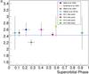 |
Fig. 1 Super-orbital dependence of the spectral index α for all MAGIC campaigns of LS I +61°303, considering a 1667-day period. The blue line corresponds to the average value. |
The dependence of α on phase with the 1667 day super-orbital period is shown in Fig. 1. The data can be fit to a constant value of 2.43 ± 0.04 (χ2/d.o.f. = 8.9/7).
We divided the dataset into intervals of high (defined as the flux being at 5–10% of the Crab Nebula flux) or low (flux at 2–5% of the Crab Nebula flux) activity. We also separated the data depending on the orbital interval of the emission into a periodical (φ = 0.5–0.75) interval, where the periodic TeV outburst occurs, and a sporadic (φ = 0.75–1.0) interval, where significant emission has been detected sporadically in the past. In neither case does the spectral index vary significantly. Fitting the data with a constant α results in an average value of 2.4 ± 0.1 (χ2/ d.o.f. = 0.90 / 2) with a probability of 0.83.
3.2. Super-orbital modulation
We performed a search for indications of a super-orbital flux modulation using the peak flux measurements at orbital phases φ = 0.5–0.75. However, some of the system’s emission peaks may have been missed, for instance, because observations can only be performed once every 24 h and because some nights were lost because of bad weather or technical problems. To minimize this effect, we only selected those measurements for which at least three consecutive observations in the requisite phase interval were successful and for which the middle time shows a higher flux than the others.
We justified this approach by simulating exactly this situation. Since observations can only be performed once every 24 h, a maximum in emission from the binary system may be missed. Additionally, observations were also lost during intervals of bad weather or technical problems. To minimize the effects of missing the maximum emission during any cycle, we only considered those orbits for which observations occurred during at least three consecutive nights in the specific phase interval. We also required that the middle observation showed the highest flux. By further assuming a shape (Landau distribution) similar to the one observed in Anderhub et al. (2009), we then calculated the percentage deviation between the actual maximum of the emission and the assigned value of the maximum. We checked that at one sigma, the difference between the estimated maximum flux level and the actual maximum was smaller than <35%, while this value increased to 90% if the maximum was used, even requiring three consecutive nights. This estimate allowed us to study the dependence of the amplitude on the orbital periodic emission observed at VHE with time.
All archival data of LS I +61°303 recorded by MAGIC since its detection in 2006 (Albert et al. 2008d, 2009; Anderhub et al. 2009; Aleksić et al. 2012a) and the data from the observing campaigns presented were folded onto the superorbital period of 1667 days. We considered statistical and systematic uncertainties in the integrated flux: 12% systematics for stereo data, according to Aleksić et al. (2012b), and 15% systematics for mono data, estimated from Albert et al. (2008c). We augmented our sample using the many observations made by VERITAS of LS I +61°303, that is, Acciari et al. (2008, 2009, 2011) and Aliu et al. (2013), using the same procedure to identify the peak of emission. We assumed 20% systematic uncertainties (Griffin 2014) that were added quadratically to the corresponding statistical uncertainties.
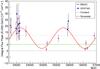 |
Fig. 2 Temporal evolution of the peak of the VHE emission for each orbital period in terms of the MJD. MAGIC (magenta dots) and VERITAS (blue squares) data within orbital phases 0.5–0.75 have been considered. The gray dashed line represents 10% of the Crab Nebula flux, the gray solid line the zero level. The fit with a sinusoidal is plotted in red and the fit with a constant in blue. |
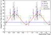 |
Fig. 3 Peak of the VHE emission in terms of the super-orbital phase defined in radio. Each data point represents the peak flux emitted in one orbital period during orbital phases 0.5–0.75 and is folded into the super-orbit of 1667 days known from radio observations (Gregory 2002). MAGIC (magenta dots) and VERITAS (blue squares) points have been used in this analysis. The fit with a sinusoidal (solid red line), with a step function (solid green line), and with a constant (solid blue line) are also represented. The gray dashed line represents 10% of the Crab Nebula flux, the gray solid line the zero level for reference. |
The temporal evolution of the peak-integrated flux above 300 GeV for each orbit is presented in Fig. 2. Folded light-curve data were fit by first assuming a hypothesis of a constant flux, and secondly assuming a sinusoidal function. The fit to a sine function yielded a period of 1610 ± 58 days with a probability of 6% (χ2/d.o.f. = 26.6/17). Since the fit probability for a constant fit is much lower, with 4.5 × 10⁻¹² (χ2/d.o.f. = 114.8/20), we can conclude that the TeV flux is variable along the superorbit and that a sinusoidal behavior with a period of 1610 days is preferred over a constant one.
Figure 3 shows the same data, but folded onto the super-orbital period of 1667 days. Here the data were fit not only with a constant and a sinusoidal, but also to two-emission levels (step function): ![\begin{eqnarray*} f(x) = \left\{\begin{array}{ccl} a & \mathrm{if} & p_1 < x < p_2, \\[\jot] b & \mathrm{if} & x < p_1 \, \& \, x > p_2, \end{array}\right. \end{eqnarray*}](/articles/aa/full_html/2016/07/aa27964-15/aa27964-15-eq55.png) where a, b, p1, and p2 are the free parameters of the fit. The results of the different fits are presented in Table 4. The probability for a constant flux is negligible, 4.5 × 10⁻¹². Assuming a sinusoidal signal, the fit probability reaches 8% (χ2/d.o.f. = 27.2/18). The fit to a step function resulted in a fit probability of 7% (χ2/d.o.f. = 26.4/17). We furthermore quantified the probability that the improvement found when fitting a sinusoid or a step function instead of a constant is produced by chance. To obtain this probability, we considered the likelihood ratio test (Mattox et al. 1996). In both cases this chance probability is <2.5 × 10⁻¹⁰, which is low. This shows that the observed intensity distribution can be described by a high and a low state and with a smoother transition. We conclude that there is a super-orbital signature in the TeV emission of LS I +61°303 and that it is compatible with the 4.5-year radio modulation seen in other frequencies.
where a, b, p1, and p2 are the free parameters of the fit. The results of the different fits are presented in Table 4. The probability for a constant flux is negligible, 4.5 × 10⁻¹². Assuming a sinusoidal signal, the fit probability reaches 8% (χ2/d.o.f. = 27.2/18). The fit to a step function resulted in a fit probability of 7% (χ2/d.o.f. = 26.4/17). We furthermore quantified the probability that the improvement found when fitting a sinusoid or a step function instead of a constant is produced by chance. To obtain this probability, we considered the likelihood ratio test (Mattox et al. 1996). In both cases this chance probability is <2.5 × 10⁻¹⁰, which is low. This shows that the observed intensity distribution can be described by a high and a low state and with a smoother transition. We conclude that there is a super-orbital signature in the TeV emission of LS I +61°303 and that it is compatible with the 4.5-year radio modulation seen in other frequencies.
3.3. Simultaneous optical-TeV observations
Correlations between the TeV flux obtained by MAGIC and the Hα parameters (EW, FWHM, and vel) measured by LIVERPOOL for the extended orbital interval 0.75–1.0.
The correlation between the TeV flux measured by MAGIC and the Hα parameters measured with the telescope (EW, FWHM, profile centroid velocity) were determined including statistical and systematic uncertainties and the weighted Pearson correlation coefficient (Soper et al. 1917).
To search for correlations, we classified the data into three different categories:
-
Simultaneous: the optical observations were performed precisely during the period when MAGIC was performing its observations. Only three such points were obtained under this condition. Because of the scarcity of such data we do not provide any correlation coefficient for this group.
-
Contemporary (hourly): data have a time difference of three hours at most.
-
Nightly: data were obtained during the same night.
Only TeV data points with a significance higher than 1σ were considered.
The data used for the correlation are given in Table 5. No statistically significant correlation was found for the sample at orbital phases φ = 0.75–1.0. A hint of a correlation is observed, but its significance is low. A stronger correlation might be blurred as a result of the fast variability of the optical parameters on short timescales compared to the long exposure times required by MAGIC, and as a result of the relatively large uncertainties and small number of data points used for this analysis. Figure 4 shows the Hα measurements plotted against the TeV flux.
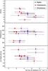 |
Fig. 4 Correlations between the TeV flux obtained by MAGIC and the Hα parameters (from top to bottom: EW, FWHM, and centroid velocity (vel)) measured by the LIVERPOOL Robotic Telescope for the orbital interval 0.75–1.0. Only TeV data points with a significance higher than 1σ have been considered. Each data point represents a ten-minute observation in the optical and a variable integration in the TeV regime: nightly (blue), contemporary (red), and strictly simultaneous data (green). Black error bars represent statistical uncertainties, while systematic uncertainties are plotted as magenta error bars. |
4. Discussion and conclusion
The main conclusions from this multi-year analysis of LS I +61°303 TeV observations are listed below.
-
1.
We achieved a first detection of super-orbital variability in the TeV regime. Using the new VHE data and the MAGIC and VERITAS archival data, we found that the super-orbital signature of LS I +61°303 is consistent with the 1667-day radio period within 8%. The TeV period obtained when fitting the data to a sine function with a free frequency instead of performing the fit as before with a fixed super-orbital period known from radio, is 1610 ± 58 days with a fit probability of 6%.
-
2.
There is no statistically significant intra-day correlation between Hα line properties and TeV emission, nor is there an obvious trend connecting the two frequencies.
The flip-flop model (Zamanov et al. 2001; Torres et al. 2012; Papitto et al. 2012) considers LS I +61°303 as a pulsar-Be star binary that changes accretion states from a propeller regime during periastron to an ejector regime at apastron. The change of state is thought to be driven by the influence of matter. The higher the pressure of this matter on the (hypothesized) neutron star magnetosphere, the more likely the latter will be compressed and disrupted. When this occurs, the pulsar wind is affected or disappears, and the inter-wind shock, which is thought to contribute to the multi-frequency non-thermal emission, disappears as well. Even when the neutron star passage at periastron is able to cut the disk off, mass accumulation will be higher in periods in which the decretion rate is higher, reaching farther out in the orbit. A larger EW of Hα may be assumed as a proxy for such a situation. If this is the case, the optical emission should be anti-correlated with the TeV flux. The detection of TeV gamma-ray super-orbital emission conforms to the predicted long-term behavior of the flip-flopping model (Torres et al. 2012). The source was found in high and low states, when expected. This result extends the earlier indications for this phenomenology found using smaller samples of TeV data (Li et al. 2012). However, we do not see this (anti-) correlation in the intra-day scales we tested. It may be that the EW of Hα is not the best tracer for decretion disk size or mass accumulation, or simply that the fast and extreme changes (by up to a factor of several in the same day) in the Hα data of the source and the vastly different integration times (minutes as compared with several hours) needed to claim a detection in both frequencies prevent us from measuring any possible trend.
Here, the reference for the periastron passage is taken at T0 = 43 366.275 MJD (Gregory 2002).
Acknowledgments
We would like to thank the Instituto de Astrofísica de Canarias for the excellent working conditions at the Observatorio del Roque de los Muchachos in La Palma. The support of the German BMBF and MPG, the Italian INFN, the Swiss National Fund SNF, and the ERDF funds under the Spanish MINECO is gratefully acknowledged. This work was also supported by the CPAN CSD2007-00042 and MultiDark CSD2009-00064 projects of the Spanish Consolider-Ingenio 2010 programme, by grant 127740 of the Academy of Finland, by the Croatian Science Foundation (HrZZ) Project 09/176, by the DFG Collaborative Research Centers SFB823/C4 and SFB876/C3, and by the Polish MNiSzW grant 745/N-HESS-MAGIC/2010/0. J.C., and D.F.T. acknowledge support by the Spanish Ministerio de Economía y Competividad (MINECO) under grant AYA2010-18080, and by MINECO and the Generalitat de Catalunya under grants AYA2012-39303 and SGR 2014-1073, respectively.
References
- Abdo, A. A., Ackermann, M., Ajello, M., et al. 2009, ApJ, 701, L123 [NASA ADS] [CrossRef] [Google Scholar]
- Acciari, V. A., Beilicke, M., Blaylock, G., et al. 2008, ApJ, 679, 1427 [NASA ADS] [CrossRef] [Google Scholar]
- Acciari, V. A., Aliu, E., Arlen, T., et al. 2009, ApJ, 700, 1034 [NASA ADS] [CrossRef] [Google Scholar]
- Acciari, V. A., Aliu, E., Arlen, T., et al. 2011, ApJ, 738, 3 [NASA ADS] [CrossRef] [Google Scholar]
- Ackermann, M., Ajello, M., Ballet, J., et al. 2013, ApJ, 773, L35 [NASA ADS] [CrossRef] [Google Scholar]
- Albert, J., Aliu, E., Anderhub, H., et al. 2006, Science, 312, 1771 [NASA ADS] [CrossRef] [PubMed] [Google Scholar]
- Albert, J., Aliu, E., Anderhub, H., et al. 2008a, Nucl. Instr. Meth. Phys. Res. A, 594, 407 [NASA ADS] [CrossRef] [Google Scholar]
- Albert, J., Aliu, E., Anderhub, H., et al. 2008b, Nucl. Instr. Meth. Phys. Res. A, 588, 424 [Google Scholar]
- Albert, J., Aliu, E., Anderhub, H., et al. 2008c, ApJ, 674, 1037 [NASA ADS] [CrossRef] [Google Scholar]
- Albert, J., Aliu, E., Anderhub, H., et al. 2008d, ApJ, 684, 1351 [NASA ADS] [CrossRef] [Google Scholar]
- Albert, J., Aliu, E., Anderhub, H., et al. 2009, ApJ, 693, 303 [NASA ADS] [CrossRef] [Google Scholar]
- Aleksić, J., Alvarez, E. A., Antonelli, L. A., et al. 2012a, ApJ, 746, 80 [NASA ADS] [CrossRef] [Google Scholar]
- Aleksić, J., Alvarez, E. A., Antonelli, L. A., et al. 2012b, Astropart. Phys., 35, 435 [NASA ADS] [CrossRef] [Google Scholar]
- Aleksic, J., Ansoldi, S., Antonelli, L. A., et al. 2015, ApJ, 927, 6505 [Google Scholar]
- Aliu, E., Anderhub, H., Antonelli, L. A., et al. 2009, Astropart. Phys., 30, 293 [NASA ADS] [CrossRef] [Google Scholar]
- Aliu, E., Archambault, S., Behera, B., et al. 2013, ApJ, 779, 88 [NASA ADS] [CrossRef] [Google Scholar]
- Anderhub, H., Antonelli, L. A., Antoranz, P., et al. 2009, ApJ, 706, L27 [NASA ADS] [CrossRef] [Google Scholar]
- Aragona, C., McSwain, M. V., Grundstrom, E. D., et al. 2009, ApJ, 698, 514 [NASA ADS] [CrossRef] [Google Scholar]
- Archibald, A. M., Stairs, I. H., Ransom, S. M., et al. 2009, Science, 324, 1411 [NASA ADS] [CrossRef] [PubMed] [Google Scholar]
- Barthelmy, S. D., Baumgartner, W., Cummings, J., et al. 2008, GRB Coordinates Network, 8215, 1 [NASA ADS] [Google Scholar]
- Burrows, D. N., Chester, M. M., D’Elia, V., et al. 2012, GRB Coordinates Network, 12914, 1 [Google Scholar]
- Casares, J., Ribas, I., Paredes, J. M., Martí, J., & Allen de Prieto, C. 2005, MNRAS, 360, 1105 [NASA ADS] [CrossRef] [Google Scholar]
- Chernyakova, M., Neronov, A., Molkov, S., et al. 2012, ApJ, 747, L29 [NASA ADS] [CrossRef] [Google Scholar]
- Dhawan, V., Mioduszewski, A., & Rupen, M. 2006, in Proc. VI Microquasar Workshop: Microquasars and Beyond, Como, Italy, 52.1 [Google Scholar]
- Fomin, V. P., Stepanian, A. A., Lamb, R. C., et al. 1994, Astropart. Phys., 2, 137 [NASA ADS] [CrossRef] [Google Scholar]
- Gregory, P. C. 2002, ApJ, 575, 427 [NASA ADS] [CrossRef] [Google Scholar]
- Griffin, S. 2014, in 2014 CAP Congress, Sudbury, Canada [Google Scholar]
- Grundstrom, E. D., & Gies, D. R. 2006, ApJ, 651, L53 [NASA ADS] [CrossRef] [Google Scholar]
- Grundstrom, E. D., Caballero-Nieves, S. M., Gies, D. R., et al. 2007, ApJ, 656, 437 [NASA ADS] [CrossRef] [Google Scholar]
- Hadasch, D., Torres, D. F., Tanaka, T., et al. 2012, ApJ, 749, 54 [NASA ADS] [CrossRef] [Google Scholar]
- Hillas, A. M. 1985, Int. Cosmic Ray Conf., 3, 445 [Google Scholar]
- Hutchings, J. B., & Crampton, D. 1981, PASP, 93, 486 [NASA ADS] [CrossRef] [Google Scholar]
- Kargaltsev, O., Rangelov, B., Hare, J., & Pavlov, G. G. 2014, Astron. Nachr., 335, 301 [NASA ADS] [CrossRef] [Google Scholar]
- Li, J., Torres, D. F., Zhang, S., et al. 2012, ApJ, 744, L13 [NASA ADS] [CrossRef] [Google Scholar]
- Li, J., Torres, D. F., & Zhang, S. 2014, ApJ, 785, L19 [NASA ADS] [CrossRef] [Google Scholar]
- Maraschi, L., & Treves, A. 1981, MNRAS, 194, 1P [NASA ADS] [CrossRef] [Google Scholar]
- Massi, M., & Torricelli-Ciamponi, G. 2014, A&A, 564, A23 [NASA ADS] [CrossRef] [EDP Sciences] [Google Scholar]
- Massi, M., Ribó, M., Paredes, J. M., et al. 2004, A&A, 414, L1 [NASA ADS] [CrossRef] [EDP Sciences] [Google Scholar]
- Mattox, J. R., Bertsch, D. L., Chiang, J., et al. 1996, ApJ, 461, 396 [NASA ADS] [CrossRef] [Google Scholar]
- Papitto, A., Torres, D. F., & Rea, N. 2012, ApJ, 756, 188 [NASA ADS] [CrossRef] [Google Scholar]
- Papitto, A., Ferrigno, C., Bozzo, E., et al. 2013, Nature, 501, 517 [NASA ADS] [CrossRef] [PubMed] [Google Scholar]
- Paredes, J. M. 1987, Ph.D. Thesis, University of Barcelona [Google Scholar]
- Paredes, J. M., Ribó, M., Bosch-Ramon, V., et al. 2007, ApJ, 664, L39 [NASA ADS] [CrossRef] [Google Scholar]
- Porter, J. M., & Rivinius, T. 2003, PASP, 115, 1153 [NASA ADS] [CrossRef] [Google Scholar]
- Rea, N., Torres, D. F., van der Klis, M., et al. 2010, MNRAS, 405, 2206 [NASA ADS] [Google Scholar]
- Reig, P. 2011, Ap&SS, 332, 1 [NASA ADS] [CrossRef] [Google Scholar]
- Soper, H. E., Young, A. W., Cave, B. M., Lee, A., & Pearson, K. 1917, Biometrika, 11, 328 [Google Scholar]
- Torres, D. F., Rea, N., Esposito, P., et al. 2012, ApJ, 744, 106 [NASA ADS] [CrossRef] [Google Scholar]
- Zamanov, R., Marti, J., & Marziani, P. 2001, in The Second National Conference on Astrophysics of Compact Objects, 50 [Google Scholar]
- Zanin, R., Carmona, E., & Sitarek, J. 2013, in Proc. ICRC 2013, Internatinal Cosmic Ray Conference [Google Scholar]
All Tables
Daily integrated flux for energies above 300 GeV of LS I +61°303 measured by MAGIC from 2010 to 2014.
Correlations between the TeV flux obtained by MAGIC and the Hα parameters (EW, FWHM, and vel) measured by LIVERPOOL for the extended orbital interval 0.75–1.0.
All Figures
|
Fig. 1 Super-orbital dependence of the spectral index α for all MAGIC campaigns of LS I +61°303, considering a 1667-day period. The blue line corresponds to the average value. |
| In the text | |
|
Fig. 2 Temporal evolution of the peak of the VHE emission for each orbital period in terms of the MJD. MAGIC (magenta dots) and VERITAS (blue squares) data within orbital phases 0.5–0.75 have been considered. The gray dashed line represents 10% of the Crab Nebula flux, the gray solid line the zero level. The fit with a sinusoidal is plotted in red and the fit with a constant in blue. |
| In the text | |
|
Fig. 3 Peak of the VHE emission in terms of the super-orbital phase defined in radio. Each data point represents the peak flux emitted in one orbital period during orbital phases 0.5–0.75 and is folded into the super-orbit of 1667 days known from radio observations (Gregory 2002). MAGIC (magenta dots) and VERITAS (blue squares) points have been used in this analysis. The fit with a sinusoidal (solid red line), with a step function (solid green line), and with a constant (solid blue line) are also represented. The gray dashed line represents 10% of the Crab Nebula flux, the gray solid line the zero level for reference. |
| In the text | |
|
Fig. 4 Correlations between the TeV flux obtained by MAGIC and the Hα parameters (from top to bottom: EW, FWHM, and centroid velocity (vel)) measured by the LIVERPOOL Robotic Telescope for the orbital interval 0.75–1.0. Only TeV data points with a significance higher than 1σ have been considered. Each data point represents a ten-minute observation in the optical and a variable integration in the TeV regime: nightly (blue), contemporary (red), and strictly simultaneous data (green). Black error bars represent statistical uncertainties, while systematic uncertainties are plotted as magenta error bars. |
| In the text | |
Current usage metrics show cumulative count of Article Views (full-text article views including HTML views, PDF and ePub downloads, according to the available data) and Abstracts Views on Vision4Press platform.
Data correspond to usage on the plateform after 2015. The current usage metrics is available 48-96 hours after online publication and is updated daily on week days.
Initial download of the metrics may take a while.