| Issue |
A&A
Volume 591, July 2016
|
|
|---|---|---|
| Article Number | A147 | |
| Number of page(s) | 6 | |
| Section | Planets and planetary systems | |
| DOI | https://doi.org/10.1051/0004-6361/201527891 | |
| Published online | 01 July 2016 | |
Charging of small grains in a space plasma: Application to Jovian stream particles
1 Universität Potsdam, Karl-Liebknecht-Str. 24/25 Building 28, 14476 Potsdam-Golm, Germany
e-mail: dzhanoev@uni-potsdam.de
2 University of Oulu, Astronomy and Space Physics, PL 3000 Oulu, Finland
Received: 4 December 2015
Accepted: 22 April 2016
Context. Most theoretical investigations of dust charging processes in space have treated the current balance condition as independent of grain size. However, for small grains, since they are often observed in space environments, a dependence on grain size is expected owing to secondary electron emission (SEE). Here, by the term “small” we mean a particle size comparable to the typical penetration depth for given primary electron energy. The results are relevant for the dynamics of small, charged dust particles emitted by the volcanic moon Io, which forms the Jovian dust streams.
Aims. We revise the theory of charging of small (submicron sized) micrometeoroids to take into account a high production of secondary electrons for small grains immersed in an isotropic flux of electrons. We apply our model to obtain an improved estimate for the charge of the dust streams leaving the Jovian system, detected by several spacecraft.
Methods. We apply a continuum model to describe the penetration of primary electrons in a grain and the emission of secondary electrons along the path. Averaging over an isotropic flux of primaries, we derive a new expression for the secondary electron yield, which can be used to express the secondary electron current on a grain.
Results. For the Jupiter plasma environment we derive the surface potential of grains composed of NaCl (believed to be the major constituent of Jovian dust stream particles) or silicates. For small particles, the potential depends on grain size and the secondary electron current induces a sensitivity to material properties. As a result of the small particle effect, the estimates for the charging times and for the fractional charge fluctuations of NaCl grains obtained using our general approach to SEE give results qualitatively different from the analogous estimates derived from the traditional approach to SEE. We find that for the charging environment considered in this paper field emission does not limit the charging of NaCl grains.
Key words: plasmas / planets and satellites: individual: Jupiter
© ESO, 2016
1. Introduction
A considerable number of mechanisms can contribute to the charging of dust grains in space. Generally, the charging process of a cosmic grain can be described by the continuity equation in integral form:  (1)where the Jk represents relevant charging currents. For spherical particles, the relation between charge qd and surface potential φd is given by qd = 4πε0aφd, provided that the grain radius a is much smaller than the plasma Debye length λd and the collisional mean free path of the plasma particles, λ, is generally larger than λd. Here ε0 = 8.854 × 10⁻¹²F m-1 is the vacuum permittivity. The currents Jk are functions of the grain properties, the ambient plasma conditions and the radiation field. At equilibrium the net current to the grain vanishes and the equilibrium grain potential φd is obtained from the flux balance equation ∑ kJk(φd(t)) = 0. It is recognized that the secondary electron emission (SEE) yield (the ratio of emitted electrons to incident ones) might be particularly important in the charging of small cosmic grains. In space, attention has focused on SEE from spacecraft surfaces or small dust particles caused by hot electrons in planetary magnetospheres (Draine & Salpeter 1979; Whipple 1981; Horányi 1992; Kempf et al. 2006). The conventional (Whipple 1981; Meyer-Vernet 1982; Horányi 1996) model for the secondary electron current Js on grains immersed in a plasma uses the approach suggested by Sternglass (1957) to estimate SEE. However, this approach is valid only in the case of big grains (semi-infinite slab model). Draine & Salpeter (1979) have shown that the secondary electron yield is enhanced when the dimensions of the grains are comparable to the primary electron penetration depth, the so-called small particle effect. Chow et al. (1993) have extended the theory suggested by Jonker (1952) to treat the small particle effect of electron impact on small spherical grains. Their model makes the simplifying but unrealistic assumption that the primary electrons are incident normal to the surface of a grain. For grains in a space plasma an isotropic incidence is more realistic. Namely, in typical magnetospheric environments in the solar system, the relative motion of a dust particle (on a Keplerian orbit) and the nearly co-rotating plasma is small, compared to the thermal velocity of the electrons. Therefore, the flux of electrons can be treated as quasi-isotropic. First attempts to include the assumption of isotropic incidence into the model of SEE from spherical grains were made by Chow (1997), and Kimura & Mann (1999). In this paper, we reconsider the formulation of a model for the secondary electron current Js on grains immersed in an isotropic flux of electrons, based on the results by Dzhanoev et al. (2015), which give a better match of experimental data than previous SEE models. In this approach we use a Maxwellian distribution of electron velocities. We illustrate our results by applying them to dust charging precesses in the Jupiter environment. Specifically, the small size effect of SEE will be important for the Jovian small particles, i.e. dust particles with radii in the range of 5nm ≤ a ≤ 15nm (for grains with speed ν> 200kms-1, Zook et al. 1996) and 30nm ≤ a ≤ 0.3μm (for grains with speed 20kms-1 ≤ ν ≤ 56kms-1, Grün et al. 1996) emanating from the Jovian system.
2. Method and model
2.1. Generalization of the SEE model
Typically, SEE depends on the material being small in metals, but often exceeding the incident flux in insulators. It has been suggested that the energy dependence of the SEE yield can be described by the Sternglass (1957) universal curve, when the yield is normalized by the maximum yield and the primary electron energy by the energy where the yield is maximized. However, a series of measurements of SEE covering a wide range of primary energies (Salow 1940; Young 1998) shows that the theory of Sternglass fails to fit the experimental data at high primary electron energy. The empirical formula developed by Draine & Salpeter (1979) generally shows a better agreement with experiments but overestimates the experimental data. Later, Chow et al. (1993) modified the yield equation by Jonker (1952) and derived the yield for secondary emission from a spherical dust grain (also for grain sizes that are comparable to the penetration depth of the primary electrons). However, their treatment was limited to the case of primary electrons that are incident normally to the grain surface. In contrast, a plasma environment in space typically provides an isotropic flux of electrons.
To describe SEE caused by isotropic incidence of primary electrons  of energy E0 on spherical objects of radius a, we consider the expression (Dzhanoev et al. 2015) for the secondary electron yield
  (2)For the evaluation of the yield we must average over the angle of incidence θ, as
  (3)Here, following Jonker (1952) we consider the case when secondary electrons are generated at a distance x from the entry location of the primary electron into a spherical grain and move to the target’s surface at an angle ϕ with direction to the nearest surface point. The Heaviside function H(2acosθ−x) selects contributions to SEE only from primaries traveling on a straight path lying entirely in the spherical grain. The parameter λ denotes the mean free path
  (4)and ϵ is the energy necessary to produce one secondary electron
 ![\begin{equation} \label{epsilonIso} \epsilon=(E_m/\delta_m)[\hat{G}_n(\bar{r}_m)/\bar{r}_m], \end{equation}](/articles/aa/full_html/2016/07/aa27891-15/aa27891-15-eq28.png) (5)where δm is the maximum yield and Em is the corresponding energy, and (Dzhanoev et al. 2015)
(5)where δm is the maximum yield and Em is the corresponding energy, and (Dzhanoev et al. 2015)  (6)The function
  has a single maximum at
  .
.  is the so-called projected range. The parameters A and n depend on the projectile and the target material and are determined by experimental measurement of R(E0), giving n = 1.5 for electrons (Fitting 1974). The distance l to the grain surface is given by
  with
with  . We note that for a spherical dust grain, ϕ can vary from 0 to ϕc = π. The angle θ between the incident direction of the primary and the normal to the surface of the grain can vary from 0 to
  . We also note that, when dealing with a grain of radius a, one can obtain from Eq. (3) an expression for the secondary electron yield valid for a semi-infinite slab by taking the limit x/a → 0.
2.2. Generalized model for the secondary electron current
In what follows, we obtain a new expression for the secondary electron current Js(φd,a) depending on grain radius, which includes the case of small grains. This expression generalizes existing expressions in the literature (Meyer-Vernet 1982, Chow et al. 1993). For a Maxwellian distribution of primary electron velocities, with the help of Eq. (3) we obtain 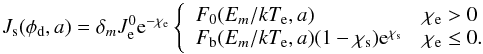 (7)Here
  and ne and
  are the number density and the mean thermal speed of the electrons. Moreover,
 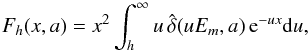 (8)where
  is the SEE yield (3) normalized by δm. Further, b = −χe/ (Em/kTe), χe,s = −eφd/kTe,s, and kTs (1−5eV) − the mean energy of the secondary electrons if their velocity distribution is also approximated by a Maxwellian distribution (Prokopenko & Laframboise 1980; Goertz 1989; Jurac et al. 1995). We assume that the charging currents are calculated by considering the orbital-motion limited (OML) theory (Laframboise & Parker 1973). In our study, we neglect the secondary emission owing to ion impact, and the reflection and backscattering of electrons and ions. In the low energy regime, the secondary electron flux cannot be approximated by a Maxwellian independently of the primary electron energy. The assumption of a Maxwell distribution for secondary electrons implies that for small incident energies a significant portion of the secondaries escape with energies greater than the incident energy. Thus, the charging calculation needs to be modified when the electron energy is tens of eV or less (Goertz 1989; Jurac et al. 1995). However, in Sect. 3.2, we show that the small particle effect is negligible for low energy primaries. So, for the purposes of our study, the modification of the charging scheme is not necessary.
3. Results and discussion
The present model (7) for the secondary electron current on spherical grains has a wide range of applicability. Here, we focus on the estimation of the electric surface potential of small dust particles in the Jupiter environment.
3.1. Plasma environment
We use the DG83 plasma model (Divine & Garrett 1983), which describes the plasma (electrons, protons and heavy ions) distributions in the Jovian magnetosphere. This model, with minor modifications, was used by Garrett et al. (2008, 2012), and will also be used here. In the following, a summary of the DG83 model is presented, which is mainly based on Divine & Garrett (1983). Three plasma populations are included in this model: radiation belt electrons and protons, warm (intermediate energy) electrons and protons, and a cold plasma population consisting of electrons, protons and typical ions found in the Jupiter system (O+, O++, S+, S++, S+++, Na+). The temperatures for warm protons and warm electrons are  , and
, and  , respectively. The temperature for cold protons and ions is the same as for cold electrons and depends on distance from Jupiter (see Sect. 3.3).
The radiation belt particles with high energy will pierce through small grains without interaction and therefore will not contribute to the charging process (Horányi and Juhász 2010). Thus, only the other two populations are considered for the charging of small grains. The DG83 model is fully three-dimensional, and the plasma distribution is described in the left-handed Jupiter System III (1965) (Seidelmann & Divine 1977). We also note that we will use this model in the orbital range [4RJ,8RJ]. In this paper, we evaluate the dust charging at fixed 110° western longitude and 0° latitude, because the plasma distribution is approximately symmetric with respect to 110° western longitude and the Jovian equator according to the formulae in Divine & Garrett (1983). We consider these plasma conditions as typical for the Jupiter environment. Two charge neutrality conditions are assumed for the DG83 model: first, the sum of the number density of cold protons and warm protons is equal to the number density of the warm electrons; second, the total charge carried by cold ions is equal to that carried by the cold electrons. To get an overall impression of the warm and cold plasma parameters (number density and temperature) used in our charging calculation, we refer to Figs. 6 and 10 in Divine & Garrett (1983).
3.2. Secondary electron emission
The dominant source of the Jovian dust streams is likely the moon Io (located at r = 5.9RJ, where RJ = 71,492km – Jupiter radius) and its volcanic activity (Graps et. al 2000). The Jovian stream particles are mainly composed of NaCl and sulphurous compounds, while silicates may be present as a minor constituent (Postberg et al. 2006). In what follows, we evaluate our grain-charging model for NaCl particles, using δm = 6 and Em = 600eV (Bruining, 1954). The bulk density for NaCl is given by ρ = 2.2 × 10³kg/m3. We also give estimate of the grain equilibrium potential for silicate particles (δm = 2.4, Em = 400eV, (Kollath, 1956), ρ = 3.3 × 10³kg/m3). The thermal energies of primary electrons are distributed according to a Maxwellian distribution.
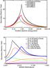 |
Fig. 1 Top: SEE yield from a NaCl grain for isotropic incidence of electrons, using typical plasma parameters for the Jovian system (see text). Grains of different radii are considered: (i) a = 0.004 μm, (ii) a = 0.01 μm, (iii) a = 0.1 μm, and (iv) 5 μm, the latter corresponding to the limit of big radius x/a → 0. Bottom: dependence of SEE yield from NaCl grains on the grain radius for various primary electron energies. On both figures the SEE yield δ(E0,a,θ = 0) induced by electrons normally incident to the grain surface is shown for comparison (Chow et al. 1993). |
Results for the case of a spherical NaCl grain are illustrated in Fig. 1. The top panel shows the secondary electron yield from single particles of different radii.
Grains with radius a = 0.1 μm and smaller exhibit a higher yield than larger grains. In the large grain limit the SEE yield converges to that from a flat surface, also revealing the universal energy dependence. The highest value for secondary electron yield is obtained when R(Em) ≈ a. This implies that, at certain values of the penetration depth R(E0), the production of secondaries is maximized. The bottom panel shows the influence of the primary electron energy on the SEE yield depending on the size of the grain. The effect of small grains becomes more pronounced as the electron energy increases from approximately 100eV to a few keV (intermediate electron energies). For small (a< 0.1 μm) grains the SEE yield does not reveal the universal dependence on energy as it is observed for large (a> 1 μm) grains and flat surfaces.
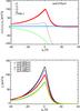 |
Fig. 2 Top: current-potential characteristics for NaCl grains with a = 0.01 μm in the Jupiter plasma environment at r ~ 5.7RJ (in the Jupiter equator and at fixed 110° western longitude, see text) with |

Thus, SEE from a spherical grain of given radius with isotropic incident flux converges in the limit of big grain radius to the case of SEE from a semi-infinite slab model. This convergence of  to δslab(E0,∞,θ = 0) is seen in the convergence of all curves to the case of 5 μm particles, which represents practically the large grain limit. We note also that there is a second peak appearing in the yield curves (Fig. 1, a = 0.1 μm), which represents an effect that is due to the finite size of grains. More detailed analysis on this topic can be found in Dzhanoev et al. (2015) and references therein. For comparison, we also show in Fig. 1 (top) and (bottom) the results for the SEE yield for the case of normally incident electrons (Chow et al. 1993). We find that, at intermediate electron energies, in the case of isotropic incidence, an electron hitting the grain obliquely is more likely to traverse the small (a ≲ 0.1 μm) grain. This reduces the SEE yield, since most secondary electrons are produced near the end of an electron path.
The approximation of the secondary electron yield by a semi-infinite slab model may work well for grains of radii a ≥ 1μm but it is not appropriate for small grains with sizes comparable or smaller than the mean depth of production of secondary electrons. So, for particles with radii from nanometers to submicrometers released from Io, the SEE yield increases with the thermal energy of plasma primary electrons kTe for low kTe<Em, it dominates when kTe is of the order of Em, and it decreases when kTe ≫ Em.
3.3. Secondary electron current and equilibrium potential
The total current versus surface potential for NaCl grains in the Jupiter plasma environment, evaluated at a distance close to Io (in the equatorial plane at 110 deg western longitude, see Sect. 3.1) is shown in Fig. 2 (top). Again, we used Eq. (3) to calculate SEE for an isotropic electron flux with Maxwellian velocity distribution. In this figure we also show all relevant currents generated by plasma electrons (Je) and ions (Ji), secondary electron production (Js) calculated via Eq. (7), and the photoelectric effect (Jn). As was shown in Fig. 1, in the limit of big grain radius (x/a → 0), the yield converges to δslab(E0,∞,θ = 0). Correspondingly, the general expression (7) for Js(φd,a) in the big grain limit converges to Js(φd,∞), calculated using a semi-infinite slab approximation for SEE, becoming independent of grain size. This convergence is shown in Fig. 2 (bottom).
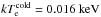
In Fig. 3 (top) we present results for the equilibrium potential φd(a) of NaCl and silicate grains derived from the flux balance condition. In Fig. 3 (i) and (iii) the calculation of φd(a) using Eq. (7) is shown. The equilibrium potential for grains with radii 1 nm ≲ a ≲ 0.1 μm differs from grains with radii a ≳ 0.1 μm and for NaCl may even be of different sign. In the curves (ii) and (iv) of Fig. 3 the equilibrium potential from a conventional approach to Js is plotted (Meyer-Vernet 1982) using the Sternglass formula. This approach does not include the small particle effect. In Fig. 3 (bottom, left) we show the dependence of the charge-to-mass ratio q/m on the grain radius. The curve (i) of Fig. 3 (bottom, left) shows the calculation of q/m using Eq. (7). The charge-to-mass ratio obtained from a conventional approach to Js is plotted in the curve (ii) of Fig. 3 (bottom, left). The results presented in the Fig. 3 (bottom, right) emphasize that the two SEE models may lead to different signs of the charge.
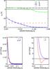 |
Fig. 3 Top: dependence of the equilibrium surface potential φd(a) on grain radius a. Materials are NaCl (i); (ii) and silicate (iii); (iv) immersed in typical plasma conditions expected at r ~ 5.7RJ distance in the Jupiter system (see text). The results (i) and (iii) are obtained from the generalized Js model (7) and compared to results (ii) and (iv) using the Sternglass approximation for SEE |

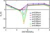 |
Fig. 4 Equilibrium potential of NaCl grains of different radii as a function of distance from Jupiter. |
In Fig. 4 we show the calculated potential for spherical grains of different radii a as a function of radial distance from Jupiter, in the range 4RJ ≤ r ≤ 8RJ. Depending on grain size the resulting equilibrium potential Φd(a,r) changes its sign. The change in sign arises from a variation of plasma parameters and the grain size dependence comes from SEE, which in turn is most sensitive to the densities and temperatures of the cold and warm electrons. The potential Φd(a,r) varies from −15 V to + 7 V. In an earlier model by Horányi (1996) the parameters δm = 1 and Em = 500eV were used, and the Sternglass formula for SEE was employed. In that framework a surface potential of Φd(r) ≈ −30V was obtained for the cold plasma torus (4RJ ≤ r ≤ 6RJ) and +3V elsewhere. In this orbital range, the plasma density peaks close to the orbit of Io (r ~ 6RJ) with  and plasma temperature has a strong minimum
  at r ~ 5RJ and rises to
  at r ~ 7.9RJ. The temperature of ions and warm electrons (for 4RJ ≤ r ≤ 8RJ) are
  and
and  respectively.
3.4. Charging time
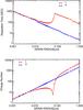 |
Fig. 5 Top: dependence of the relaxation time τd for charge deviations on the grain’s radius a. The results presented for NaCl grains immersed in typical plasma conditions expected at r ~ 5.7RJ distance in the Jupiter system (see text). The result (i) is obtained for the generalized Js model (7) and compared to results (ii) obtained using the Sternglass approximation for SEE. Bottom: dependence of the charge number |⟨N⟩| on grain’s radius a with the same parameters and notation as for Fig. 5 (top). |
In Fig. 5 (top) we present results for the charging times τd(a) of NaCl grain of different radii. Because the fastest charging occurs for high plasma densities in a close vicinity to Io, the results in Fig. 5 (top) could be considered as a reasonable estimate of the lower limit for τd(a) of NaCl grains in the Jupiter plasma environment (in the orbital range [4RJ,8RJ]). In the curve (i) of Fig. 5 (top) the calculation of τd(a) using Eq. (7) is shown. In the curve (ii) of Fig. 5 (top) the charge relaxation time from a conventional approach to Js is plotted (Meyer-Vernet 1982). From the curve (i) of Fig. 5 (top), we see that the small particle effect modifies the well-known size dependence τd ~ a-1 relevant for the case described by the curve (ii). Thus, the different SEE models lead to different charging times.
3.5. Estimate of charge fluctuations
Because of the statistical nature of the collection currents, the calculated charge on the NaCl grain is not fixed, but it can fluctuate around its equilibrium value q (Ciu & Goree 1994; Meier et al. 2014, 2015). The charge fluctuation may also be in response to varying conditions in the Jupiter plasma environment. The quantized grain charging corresponds to a Poisson process (Khrapak et al. 1999; Hsu et al. 2011) are shown and the resulting distribution of charge fluctuations has the shape of a Gaussian with ⟨qd⟩ ~ q (Yaroshenko & Lühr 2014). Based on Poisson statistics (Ciu & Goree 1994, Khrapak et al. 1999), the fractional charge fluctuation were obtained, which varies as Δqd/ ⟨qd⟩ ~ |⟨N⟩|− 1/2, where ⟨N⟩ = ⟨qd/e⟩ is the charge number obtained from the continuous charging model. In the curve (i) of Fig. 5 (bottom), the charge number ⟨N⟩ from a conventional approach to Js is plotted. In the curve (ii) of Fig. 5 (bottom), we show results for the Sternglass model for SEE. From curve (ii) of Fig. 5 (bottom), the |⟨N⟩|− 1/2 scaling means that smaller nano-sized NaCl grains may have larger fractional charge fluctuation levels. However, from the curve (i) of Fig. 5 (bottom) we see that for our generalized Js model (7) the NaCl grains with radii close to a ~ 3 nm and a ~ 60 nm have comparable values of the charge number |⟨N⟩|. Thus, the small particle effect modifies the dependence of the fractional charge fluctuations Δqd/ ⟨qd⟩ on the grain size.
3.6. Field emission and grain charge limitation
Even a relatively small charge on a grain of small size may induce a large surface electric field, which significantly modifies the potential barrier at the surface (Mendis & Axford 1974). So, the high-field processes of electron or ion field emissions, in general, have to be taken into account (Jeřáb et al. 2010; Meyer-Vernet 2013).
The electric field may be high enough to eject electrons from the grain surface. This may limit the negative charge of the grain. The electron field emission limit of surface electric field (|E| = |φd| /a) is about 103V /μm (Gomer 1961). This corresponds to the limiting potential φef ≈ −1V(a/ 1 nm), which is equivalent to a limiting grain charge qfe ~ −0.7e(a/ 1nm)2. For instance, for grains with a< 1.7nm, we have |⟨N⟩| < 2, and the grain charge is limited to one single electron. For grains with a< 0.1 μm and a< 1 μm, we get |⟨N⟩| | < 7 × 10³ and |⟨N⟩| < 7 × 10⁵. Thus, as can be seen from the results in Fig. 4 and, in particular, from the curve (i) of Fig. 5 (bottom), the negatively charged NaCl grains of radii a ≳ 60nm have an equilibrium charge that is much lower than the limiting charge. So, the field electron emission does not show an effect for the NaCl grains. The field ion emission, which limits the positive charging, requires a much higher field than the field electron emission ~104V /μm (Good & Müller 1956), which corresponds to the limiting potential φif ≈ + 10 V(a/ 1 nm). Accordingly, for positively charged grains with a ≲ 60nm, we have |⟨N⟩| ≲ 2.5 × 10⁴. Thus, from the results in Fig. 4, it follows that the ion field emission does not show an effect for positively charged NaCl grains also.
4. Conclusions
In this study, we have revised the treatment of the charging of small grains immersed in an isotropic flux of electrons. For this purpose, we obtained a new model for the secondary electron current Js owing to a generalization of the SEE model that is valid for small grains immersed in an isotropic flux of electrons. Furthermore, we qualitatively and quantitatively show how the results differ from widely used conventional models for the SEE yield. Our generalization of the charging model is important for dust grain sizes that are typically found in circumplanetary environments.
Employing plasma conditions for the Jovian system, we find that, for small (a ≤ 1 μm) particles, the grain potential φd depends on grain size, while this is independent of size for big (a ≥ 1 μm) particles. This effect may have important consequences for circumplanetary dust:
-
two grains (or parts of a more complex body), with the samecomposition and shape in the same environment and with thesame history, can have different charges, depending on their sizesand, in extreme cases, they can have charges of the opposite sign;
-
the grain potential may significantly differ depending on grain size;
-
the new SEE model leads to estimates of charging times that are qualitatively different from similar estimates derived from the traditional SEE model;
-
nano-sized and submicron sized grains may have comparable fractional charge fluctuations;
-
field emission does not limit the grain charge.
We also show that the charging in the Jupiter environment is particularly sensitive to the dust particle’s material properties. Because the dynamics of grains in the range between 10 nm to 100 nm is dominated by the electromagnetic field, the precise value of the grain charge has a strong effect for particle transport and ejection from the Jovian system. We used our generalization of the charging model to estimate the surface potential of dust grains in the Jupiter environment but the results have a wider range of applicability and can be relevant for many charging processes where secondary electron currents are involved.
Acknowledgments
We thank the anonymous referee for important comments that improved the content of this paper. This work was supported by German Deutsche Forschungsgemeinschaft, DFG project through Schwerpunktprogramm 1488 Planet Mag (Grant SCHM 1642/2–1) and by European Space Agency (ESA), funding project Jovian Meteoroid Environment Model (JMEM, contract number: 4000107249/12/NL/AF).
References
- Bruining, H. 1954, Physics and Applications of Secondary Electron Emission (London: Pergamon Press) [Google Scholar]
- Ciu, C., & Goree, J. 1994, Plasma Sci., IEEE Trans., 22, 151 [Google Scholar]
- Chow, V. W. 1997, in Adv. in Dusty Plasmas, eds. P. K. Shukla, D. A. Mendis, & T. Desai (Singapore: World Scientific), 77 [Google Scholar]
- Chow, V. W., Mendis, D. A., & Rosenberg, M. 1993, J. Geophys. Res., 98, 19065 [NASA ADS] [CrossRef] [Google Scholar]
- Divine, N., & Garrett, H. B. 1983, J. Geophys. Res.: Space Phys. (1978–2012), 88, 6889 [NASA ADS] [CrossRef] [Google Scholar]
- Draine, B. T., & Salpeter, E. E. 1979, ApJ, 231, 77 [NASA ADS] [CrossRef] [Google Scholar]
- Dzhanoev, A. R., Spahn, F., Yaroshenko, V., Lühr, H., & Schmidt, J. 2015, Phys. Rev. B, 92, 125430 [NASA ADS] [CrossRef] [Google Scholar]
- Fitting, H.-J. 1974, Phys. Status Solidi, 26, 525 [NASA ADS] [CrossRef] [Google Scholar]
- Garrett, H. B., Evans, R. W., Whittlesey, A. C., Katz, I., & Jun, I. 2008, Plasma Sci., IEEE Trans., 36, 2440 [Google Scholar]
- Garrett, H. B., Katz, I., Jun, I., et al. 2012, Plasma Sci., IEEE Trans., 40, 144 [Google Scholar]
- Goertz, C.K. 1989, Rev. Geophys., 27, 271 [NASA ADS] [CrossRef] [Google Scholar]
- Gomer, R. 1961, Field Emission and Field Ionisation (Cambridge, Mass.: Harvard Univ. Press) [Google Scholar]
- Good, R. & Müller, E. 1956, Encyclopedia of Physics, Vol. XXI (Springer-Verlag) [Google Scholar]
- Graps, A. L., Grün, E., Svedhem, H., et al. 2000, Nature, 405, 48 [NASA ADS] [CrossRef] [Google Scholar]
- Grün, E., Baguhl, M., Hamilton, D. P., Riemann, R., Zook, H. A., et al. 1996, Nature, 381, 395 [NASA ADS] [CrossRef] [Google Scholar]
- Horányi, M. 1996, An. Rev. Astrophys., 34, 383 [Google Scholar]
- Horányi, M., & Juhász, A. 2010, J. Geophys. Res.: Space Phys. (1978–2012), 115, A9 [Google Scholar]
- Horányi, M., Burns, J. A., & Hamilton, D. 1992, Icarus, 97, 248 [NASA ADS] [CrossRef] [Google Scholar]
- Hsu, H.-W., Postberg, F., Kempf, S., et al. 2011, J. Geophys. Res.: Space Phys. 116, 9215 [Google Scholar]
- Jeřáb, M., Vaverka, J., Vyšinska, M., et al. 2010, Plasma Sci., IEEE Trans., 38, 798 [Google Scholar]
- Jonker, J. L. H. 1952, Philips Res. Rep., 7, 1 [Google Scholar]
- Jurac, S., Baragiola, R. A., Johnson, R. E., & Sittler Jr, E. C. 1995, J. Geophys. Res., 100, 14821 [NASA ADS] [CrossRef] [Google Scholar]
- Kempf, S., Beckmann, U., Srama, R., et al. 2006, Planet. Space Sci., 54, 999 [NASA ADS] [CrossRef] [Google Scholar]
- Khrapak, S. A., Nefedov, A. P., Petrov, O. F., & Vaulina, O. S. 1999, Phys. Rev. E, 59, 6017 [NASA ADS] [CrossRef] [Google Scholar]
- Kimura, H., & Mann, I. 1999, Earth Planets Space, 51, 1223 [NASA ADS] [CrossRef] [Google Scholar]
- Kollath, R. 1956, in Electron Emission, Gas discharges I, ed. S. Flügge (Berlin: Springer-Verlag) 232 [in German] [Google Scholar]
- Laframboise, J. G., & Parker, L. W. 1973, Phys. Fluids, 16, 629 [NASA ADS] [CrossRef] [Google Scholar]
- Meier, P., Kriegel, H., Motschmann, U., et al. 2014, Planet. Space Sci., 104, 216 [NASA ADS] [CrossRef] [Google Scholar]
- Meier, P., Motschmann, U., Schmidt, J., et al. 2015, Planet. Space Sci., 119, 208 [NASA ADS] [CrossRef] [Google Scholar]
- Mendis, D. A., & Axford, W. I. 1974, Ann. Rev. Earth Planet. Sci., 2, 419 [NASA ADS] [CrossRef] [Google Scholar]
- Meyer-Vernet, N. 1982, A&A, 105, 98 [NASA ADS] [Google Scholar]
- Meyer-Vernet, N. 2013, Icarus, 226, 583 [NASA ADS] [CrossRef] [Google Scholar]
- Postberg, F., Kempf, S., Srama, R., et al. 2006, Icarus, 183, 1 [NASA ADS] [CrossRef] [Google Scholar]
- Prokopenko, S. M. L., & Laframboise, J. G. 1980, J. Geophys. Res., 85, 4125 [NASA ADS] [CrossRef] [Google Scholar]
- Salow, H. 1940, Zeitschr. Tech. Physik, 21, 8 [in German] [Google Scholar]
- Seidelmann, P. K., & Divine, N. 1977, Geophys. Res. Lett., 4, 65 [NASA ADS] [CrossRef] [Google Scholar]
- Sternglass, E. J. 1957, Phys. Rev., 108, 1 [NASA ADS] [CrossRef] [Google Scholar]
- Whipple, E. C. 1981, Rep. Prog. Phys., 44, 1197 [NASA ADS] [CrossRef] [Google Scholar]
- Yaroshenko, V. V., & Lühr, H. 2014, J. Geophys. Res.: Space Phys., 119, 6190 [NASA ADS] [CrossRef] [Google Scholar]
- Young, Y. C., Thong, J. T. L., & Phang, J. C. H. 1998, J. Appl. Phys., 84, 4543 [NASA ADS] [CrossRef] [Google Scholar]
- Zook, H. A., Grün, E., Baguhl, M., et al. 1996, Science, 274, 5292 [Google Scholar]
All Figures
|
Fig. 1 Top: SEE yield from a NaCl grain for isotropic incidence of electrons, using typical plasma parameters for the Jovian system (see text). Grains of different radii are considered: (i) a = 0.004 μm, (ii) a = 0.01 μm, (iii) a = 0.1 μm, and (iv) 5 μm, the latter corresponding to the limit of big radius x/a → 0. Bottom: dependence of SEE yield from NaCl grains on the grain radius for various primary electron energies. On both figures the SEE yield δ(E0,a,θ = 0) induced by electrons normally incident to the grain surface is shown for comparison (Chow et al. 1993). |
| In the text | |
|
Fig. 2 Top: current-potential characteristics for NaCl grains with a = 0.01 μm in the Jupiter plasma environment at r ~ 5.7RJ (in the Jupiter equator and at fixed 110° western longitude, see text) with |
| In the text | |
|
Fig. 3 Top: dependence of the equilibrium surface potential φd(a) on grain radius a. Materials are NaCl (i); (ii) and silicate (iii); (iv) immersed in typical plasma conditions expected at r ~ 5.7RJ distance in the Jupiter system (see text). The results (i) and (iii) are obtained from the generalized Js model (7) and compared to results (ii) and (iv) using the Sternglass approximation for SEE |
| In the text | |
|
Fig. 4 Equilibrium potential of NaCl grains of different radii as a function of distance from Jupiter. |
| In the text | |
|
Fig. 5 Top: dependence of the relaxation time τd for charge deviations on the grain’s radius a. The results presented for NaCl grains immersed in typical plasma conditions expected at r ~ 5.7RJ distance in the Jupiter system (see text). The result (i) is obtained for the generalized Js model (7) and compared to results (ii) obtained using the Sternglass approximation for SEE. Bottom: dependence of the charge number |⟨N⟩| on grain’s radius a with the same parameters and notation as for Fig. 5 (top). |
| In the text | |
Current usage metrics show cumulative count of Article Views (full-text article views including HTML views, PDF and ePub downloads, according to the available data) and Abstracts Views on Vision4Press platform.
Data correspond to usage on the plateform after 2015. The current usage metrics is available 48-96 hours after online publication and is updated daily on week days.
Initial download of the metrics may take a while.