© ESO, 2016

1. Introduction

The origin and evolution of cosmic magnetism are at present poorly understood. Answering the many open questions surrounding the physics of astrophysical magnetic fields is a difficult task since magnetic fields can be significantly affected by structure and galaxy formation and evolutionary processes. Their strength can be amplified, for example, in galaxy clusters through mergers and in galaxies through large-scale dynamos, invoking differential rotation and turbulence. Insights into the origin and properties of magnetic fields in the Universe could be provided by probing them on even larger scales. Along filaments and voids of the cosmic web, turbulent intracluster gas motions have not yet enhanced the magnetic field; its strength thus still depends on the seed field intensity, in contrast to galaxy clusters, where it probably mostly reflects the present level of turbulence (see, e.g., Donnert et al. 2009; Xu et al. 2010, 2011). Intervening magnetoionic media cause a difference in the phase velocity between the left-handed and right-handed circular polarization components of the linearly polarized synchrotron radiation emitted by a background radio source (e.g., Carilli & Taylor 2002; Govoni & Feretti 2004). This effect translates into a rotation of the intrinsic polarization angle, ψ₀, $\mathit{\psi }\mathrm{\left(}{\mathit{\lambda }}^{\mathrm{2}}\mathrm{\right)}\mathrm{=}{\mathit{\psi }}_{\mathrm{0}}\mathrm{+}\mathit{\phi }{\mathit{\lambda }}^{\mathrm{2}}\mathit{.}$(1)Following Burn (1966), the observed polarization angle, ψ, depends on the observation wavelength, λ, through the Faraday depth, φ, $\mathit{\phi }\mathrm{=}{\mathit{a}}_{\mathrm{0}}{\mathrm{\int }}_{\mathrm{0}}^{{\mathit{z}}_{\mathrm{s}}}{\mathit{B}}_{\mathit{l}}\mathrm{\left(}\mathit{z}\mathrm{\right)}{\mathit{n}}_{\mathrm{e}}\mathrm{\left(}\mathit{z}\mathrm{\right)}\frac{\mathrm{d}\mathit{l}}{\mathrm{d}\mathit{z}}\mathrm{d}\mathit{z,}$(2)where a₀ depends only on fundamental constants, n_e is the electron density, B_l is the component of the magnetic field along the line of sight, and z_s is the redshift of the source. When the rotation is completely due to a foreground screen, the Faraday depth has the same value as the rotation measure (RM), defined by $\mathrm{RM}\mathrm{\equiv }\frac{\mathit{\partial \psi }}{\mathit{\partial }{\mathit{\lambda }}^{\mathrm{2}}}\mathrm{·}$(3)The Faraday depth is assumed to be positive when the line-of-sight average component of the magnetic field points toward the observer, otherwise it is negative for a field with an average component pointing away from the observer. The amount of Faraday depth measured by radio observations along a given line of sight is the sum of the contributions from the Milky Way, the emitting radio source, and any other source and large-scale structure in between hosting a magnetized plasma. The investigation of these contributions and of their possible dependence on redshift is essential to discriminate among the different scenarios of magnetic field formation and evolution and, therefore, crucial for the understanding of cosmic magnetism. Sensitive observations, a good knowledge of the Galactic Faraday foreground screen, and a statistical approach that is able to properly combine all of the observational information are necessary. An all-sky map of the Galactic Faraday rotation foreground and an estimate of the overall extragalactic contribution has been derived by Oppermann et al. (2012, 2015) in the framework of “Information Field Theory” (Enßlin et al. 2009) by assuming a correlated Galactic foreground and a completely uncorrelated extragalactic term. In this paper, we propose a new, fully Bayesian approach aiming at further disentangling the contribution intrinsic to emitting sources from the contribution due to the intergalactic environment between the source and the observer and at investigating the dependence of these contributions on redshift.

The first direct proof of the existence of magnetic fields in large-scale extragalactic environments, i.e., galaxy clusters, dates back to the 1970s with the discovery of extended, diffuse, central synchrotron sources called radio halos (see, e.g., Feretti et al. 2012 for a review). Later, indirect evidence of the existence of intracluster magnetic fields has been given by several statistical studies on the effect of the Faraday rotation on the radio signal from background galaxies or galaxies embedded in galaxy clusters (Lawler & Dennison 1982; Vallée et al. 1986; Clarke et al. 2001; Johnston-Hollitt 2003; Clarke 2004; Johnston-Hollitt & Ekers 2004). On scales up to a few Mpc from the nearest galaxy cluster, possibly along filaments, only a few diffuse synchrotron sources have been reported (Harris et al. 1993; Bagchi et al. 2002; Kronberg et al. 2007; Giovannini et al. 2013, 2015). Magnetic fields with strengths on the order of 10^-15 G in voids might be indicated by γ-ray observations (see Neronov & Vovk 2010; Tavecchio et al. 2010; Takahashi et al. 2012, 2013; but see Broderick et al. 2014a,b for alternative possibilities). Nevertheless, up to now, a robust confirmed detection of magnetic fields on scales that are much larger than clusters is not available. Stasyszyn et al. (2010) and Akahori et al. (2014a) investigated the possibility of statistically measuring Faraday rotation from intergalactic magnetic fields with present observations, showing that only the Square Kilometre Array (SKA) and its pathfinders are likely to succeed in this respect. By comparing the observations with single-scale magnetic field simulations, Pshirkov et al. (2015) infer an upper limit of 1.2 nG for extragalactic large-scale magnetic fields, while the Planck Collaboration XIX (2016) derived a more stringent upper limit for primordial large-scale magnetic fields of B< 0.67 nG from the analysis of the Cosmic Microwave Background (CMB) power spectra and the effect on the ionization history (but see also Takahashi et al. 2005; Ichiki et al. 2006).

A number of authors examined a possible dependence of extragalactic Faraday depths on the redshift of the observed radio source, but no firm conclusion has yet been drawn. Kronberg & Perry (1982) found an increased variance of the Faraday depth in conjunction with higher redshifts, as also found in some later studies (e.g., Welter et al. 1984; Kronberg et al. 2008). However, Oren & Wolfe (1995) did not find any evidence of an increase of the variance of the Faraday depth as a function of the redshift, as also suggested by the recent work by Hammond et al. (2012) and Pshirkov et al. (2015).

The rest of this paper is organized as follows. In Sect. 2, we describe the theory behind our method. In Sect. 3, the tests performed are presented with predictions for the new generation of radio interferometers. Moreover, we outline a generalization of the algorithm in order to discriminate the contribution from different large-scale structures along the line of sight. Finally, in Sect. 4, we draw our conclusions. The application of the algorithm to real data is left for future work, as explained in the text. In the following, we adopt a ΛCDM cosmology with H₀ = 67.3 km s^-1Mpc^-1, Ω_m = 0.315, Ω_Λ = 0.685, and Ω_c = 0.0 (Planck Collaboration XVI 2014).

2. Theoretical framework

The probability for the extragalactic contribution, φ_e, along the line of sight, i, to take on a value within the infinitesimal interval between φ_e,i and φ_e,i + dφ_e,i given the data, d, and a model parameterization, Θ, is given by the probability density distribution. As shown by Oppermann et al. (2015), the prior probability density distribution of the extragalactic Faraday depth can be approximated with a Gaussian. The mean and variance, 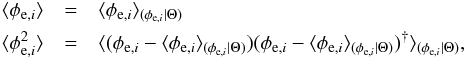$\begin{array}{ccc}\mathrm{⟨}{\mathit{\phi }}_{\mathrm{e}\mathit{,i}}\mathrm{⟩}& \mathrm{=}& \mathrm{⟨}{\mathit{\phi }}_{\mathrm{e}\mathit{,i}}{\mathrm{⟩}}_{\mathrm{\left(}{\mathit{\phi }}_{\mathrm{e}\mathit{,i}}\mathrm{\right|}\mathrm{\Theta }\mathrm{)}}\\ \mathrm{⟨}{\mathit{\phi }}_{\mathrm{e}\mathit{,i}}^{\mathrm{2}}\mathrm{⟩}& \mathrm{=}& \mathrm{⟨}\mathrm{(}{\mathit{\phi }}_{\mathrm{e}\mathit{,i}}\mathrm{-}\mathrm{⟨}{\mathit{\phi }}_{\mathrm{e}\mathit{,i}}{\mathrm{⟩}}_{\mathrm{\left(}{\mathit{\phi }}_{\mathrm{e}\mathit{,i}}\mathrm{\right|}\mathrm{\Theta }\mathrm{)}}\mathrm{)}\mathrm{(}{\mathit{\phi }}_{\mathrm{e}\mathit{,i}}\mathrm{-}\mathrm{⟨}{\mathit{\phi }}_{\mathrm{e}\mathit{,i}}{\mathrm{⟩}}_{\mathrm{\left(}{\mathit{\phi }}_{\mathrm{e}\mathit{,i}}\mathrm{\right|}\mathrm{\Theta }\mathrm{)}}{\mathrm{)}}^{†}{\mathrm{⟩}}_{\mathrm{\left(}{\mathit{\phi }}_{\mathrm{e}\mathit{,i}}\mathrm{\right|}\mathrm{\Theta }\mathrm{)}}\mathit{,}\end{array}$(4)of this distribution are 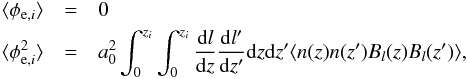$\begin{array}{ccc}\mathrm{⟨}{\mathit{\phi }}_{\mathrm{e}\mathit{,i}}\mathrm{⟩}& \mathrm{=}& \mathrm{0}\\ \mathrm{⟨}{\mathit{\phi }}_{\mathrm{e}\mathit{,i}}^{\mathrm{2}}\mathrm{⟩}& \mathrm{=}& \end{array}$(5)where these averages are calculated with respect to the prior of the extragalactic Faraday depth P(φ_e,i | Θ). The zero mean results from the fact that we do not have any reason to suppose either a positive or a negative mean Faraday depth value. Frozen-in magnetic fields are expected to have strengths depending on redshift z. Because of the expansion of the Universe, lengths are stretched $\frac{{\mathit{l}}_{\mathrm{0}}}{\mathit{l}}\mathrm{=}\mathrm{(}\mathrm{1}\mathrm{+}\mathit{z}\mathrm{)}\mathit{.}$(6)In an isotropically expanding Universe with no significant fluctuations, the mean electron density evolves as $\frac{\mathrm{⟨}{\mathit{n}}_{\mathrm{e}}\mathrm{⟩}}{\mathrm{⟨}{\mathit{n}}_{\mathrm{0}}\mathrm{⟩}}\mathrm{=}\mathrm{(}\mathrm{1}\mathrm{+}\mathit{z}{\mathrm{)}}^{\mathrm{3}}\mathit{,}$(7)and, if the magnetic flux density is conserved, the magnetic field strength as $\frac{\mathrm{⟨}\mathit{B}\mathrm{⟩}}{\mathrm{⟨}{\mathit{B}}_{\mathrm{0}}\mathrm{⟩}}\mathrm{=}{\left(\frac{\mathrm{⟨}{\mathit{n}}_{\mathrm{e}}\mathrm{⟩}}{\mathrm{⟨}{\mathit{n}}_{\mathrm{0}}\mathrm{⟩}}\right)}^{\frac{\mathrm{2}}{\mathrm{3}}}\mathrm{=}\mathrm{(}\mathrm{1}\mathrm{+}\mathit{z}{\mathrm{)}}^{\mathrm{2}}\mathit{,}$(8)where l₀, ⟨ n₀ ⟩, and ⟨ B₀ ⟩ are the present-day values, and l, ⟨ n_e ⟩, and ⟨ B ⟩ are the values at the time when the signal was emitted by the source. If we consider these assumptions and we define a length scale Λ_l: = ^∫dl′ ⟨ B(l)B(l′) ⟩ / ⟨ B(l)² ⟩, we obtain $\mathrm{⟨}{\mathit{\phi }}_{\mathrm{e}\mathit{,i}}^{\mathrm{2}}\mathrm{⟩}\mathrm{\approx }{\mathit{a}}_{\mathrm{0}}^{\mathrm{2}}{\mathrm{\int }}_{\mathrm{0}}^{{\mathit{z}}_{\mathit{i}}}\mathrm{⟨}{\mathit{n}}_{\mathrm{0}}^{\mathrm{2}}\mathrm{⟩}\mathrm{⟨}{\mathit{B}}_{\mathit{l}\mathrm{0}}^{\mathrm{2}}\mathrm{⟩}{\mathrm{\Lambda }}_{\mathit{l}\mathrm{0}}\mathrm{(}\mathrm{1}\mathrm{+}\mathit{z}{\mathrm{)}}^{\mathrm{4}}\frac{\mathit{c}}{\mathit{H}\mathrm{\left(}\mathit{z}\mathrm{\right)}}\mathrm{d}\mathit{z}\mathit{.}$(9)For the derivation of this expression, see Appendix A. Here, we assumed an unstructured Universe¹ and used the definition of proper displacement along a light ray, $\frac{\mathrm{d}\mathit{l}}{\mathrm{d}\mathit{z}}\mathrm{=}\frac{\mathit{c}}{\mathrm{(}\mathrm{1}\mathrm{+}\mathit{z}\mathrm{)}\mathit{H}\mathrm{\left(}\mathit{z}\mathrm{\right)}}$. Moreover, we assumed that, within a correlation length Λ_l0, the redshift can be approximated to be constant. Magnetic field strength and structure and the electron density have different values in different environments, j. In the following, we assume them to depend only on the environment and not on the location within an environment. This simplification renders the problem feasible. The letters i and j should not be mixed up since they have a different meaning. Indeed, they refer to the line of sight and to the environment (e.g., galaxy clusters, voids, filaments, and sheets.), respectively.

In this paper, as a first step, we restrict our analysis to two components (scenario 2C): the emitting radio source itself, whose contribution is ${\mathit{\sigma }}_{\mathrm{int}\mathit{,i}}^{\mathrm{2}}\mathrm{\left(}{\mathit{z}}_{\mathit{i}}\mathit{,}\mathrm{\Theta }\mathrm{\right)}$, and the medium between the source and our Galaxy, whose contribution is ${\mathit{\sigma }}_{\mathrm{env}\mathit{,i}}^{\mathrm{2}}\mathrm{\left(}{\mathit{z}}_{\mathit{i}}\mathit{,}\mathrm{\Theta }\mathrm{\right)}$, such that $\mathrm{⟨}{\mathit{\phi }}_{\mathrm{e}\mathit{,i}}^{\mathrm{2}}\mathrm{⟩}\mathrm{=}{\mathit{\sigma }}_{\mathrm{e}\mathit{,i}}^{\mathrm{2}}\mathrm{\left(}{\mathit{z}}_{\mathit{i}}\mathit{,}\mathrm{\Theta }\mathrm{\right)}\mathrm{=}{\mathit{\sigma }}_{\mathrm{int}\mathit{,i}}^{\mathrm{2}}\mathrm{\left(}{\mathit{z}}_{\mathit{i}}\mathit{,}\mathrm{\Theta }\mathrm{\right)}\mathrm{+}{\mathit{\sigma }}_{\mathrm{env}\mathit{,i}}^{\mathrm{2}}\mathrm{\left(}{\mathit{z}}_{\mathit{i}}\mathit{,}\mathrm{\Theta }\mathrm{\right)}\mathit{.}$(10)We denote with Θ = { σ_int,0,σ_env,0,χ_lum,χ_red } an N-dimensional vector, where N is the number of parameters used in the representation of the Faraday depth variance. These are the parameters we want to infer: σ_int,0 is the pure Faraday depth variance intrinsic to the emitting radio source, σ_env,0 is the pure large-scale Faraday depth variance, χ_lum describes the luminosity dependence of the intrinsic contribution, and χ_red describes the redshift dependence of the large-scale contribution. We choose the following parameterization for the intrinsic contribution to the variance in Faraday depth, ${\mathit{\sigma }}_{\mathrm{int}\mathit{,i}}^{\mathrm{2}}\mathrm{\left(}{\mathit{z}}_{\mathit{i}}\mathit{,}\mathrm{\Theta }\mathrm{\right)}\mathrm{=}{\left(\frac{{\mathit{L}}_{\mathit{i}}}{{\mathit{L}}_{\mathrm{0}}}\right)}^{{\mathit{\chi }}_{\mathrm{lum}}}\frac{{\mathit{\sigma }}_{\mathrm{int}\mathit{,}\mathrm{0}}^{\mathrm{2}}}{\mathrm{(}\mathrm{1}\mathrm{+}{\mathit{z}}_{\mathit{i}}{\mathrm{)}}^{\mathrm{4}}}\mathit{,}$(11)where L_i is the total luminosity² of the source i, L₀ = 10²⁷ W/Hz, and χ_lum absorbs possible dependencies on the luminosity of the source since faint sources may not be detected. In a flux-limited catalog, only the brightest sources are detected in the distant Universe. This selection effect can bias the evaluation of the contribution intrinsic to the source, e.g., if the Faraday depth associated with bright sources differs from that in faint sources. We take this possible effect into account with χ_lum. Alternatively, a parameterization based on polarized luminosity would also be a reasonable choice. For the environmental contribution, we choose as a parameterization ${\mathit{\sigma }}_{\mathrm{env}\mathit{,i}}^{\mathrm{2}}\mathrm{\left(}{\mathit{z}}_{\mathit{i}}\mathit{,}\mathrm{\Theta }\mathrm{\right)}\mathrm{=}\frac{{\mathit{D}}_{\mathit{i}}\mathrm{\left(}{\mathit{z}}_{\mathit{i}}\mathit{,}{\mathit{\chi }}_{\mathrm{red}}\mathrm{\right)}}{{\mathit{D}}_{\mathrm{0}}}{\mathit{\sigma }}_{\mathrm{env}\mathit{,}\mathrm{0}}^{\mathrm{2}}\mathit{,}$(12)where D₀ = 1 Gpc, and D_i(z,χ_red) is defined as ${\mathit{D}}_{\mathit{i}}\mathrm{\left(}{\mathit{z}}_{\mathit{i}}\mathit{,}{\mathit{\chi }}_{\mathrm{red}}\mathrm{\right)}\mathrm{=}{\mathrm{\int }}_{\mathrm{0}}^{{\mathrm{z}}_{\mathrm{i}}}\frac{\mathit{c}}{\mathit{H}\mathrm{\left(}\mathit{z}\mathrm{\right)}}\mathrm{(}\mathrm{1}\mathrm{+}\mathit{z}{\mathrm{)}}^{\mathrm{4}\mathrm{+}{\mathit{\chi }}_{\mathrm{red}}}\mathrm{d}\mathit{z}$(13)to capture the redshift scaling of Eq. (9). We derived this redshift dependence assuming an isotropically expanding Universe with no significant fluctuations. Possible deviations from this simplistic scenario are taken into account by the parameter χ_red. Since the length of the path covered by the signal in the source is not known for each source, we factored it in ${\mathit{\sigma }}_{\mathrm{int}\mathit{,}\mathrm{0}}^{\mathrm{2}}$ in Eq. (11). We note that σ_int,0 and σ_env,0 were assumed to be independent of the redshift. In Eq. (11) the only redshift dependence is absorbed by the factor (1 + z_i)^-4 that takes into account the effect of redshift on Faraday rotation (squared), while in Eq. (12) it is absorbed by D_i(z_i,χ_red), which is given in Eq. (13).

This parameterization describes the simplest scenario. For more complex scenarios that include three components, we refer to Appendix C, where we introduce an additional constant and latitude-dependent term. Moreover, galaxies along the line of sight between a source and the observer can be responsible for high Faraday depth values (e.g., Kronberg & Perry 1982; Welter et al. 1984; Kronberg et al. 2008; Bernet et al. 2012), indicating magnetic field strengths in these intervening galaxies of (1.8±0.4) μG (Farnes et al. 2014a). The rotation of the polarization angle due to these sources adds to that associated with the large-scale structure and, therefore, should be taken into account in a proper modeling. Since the aim of this paper is to give a proof of concept, we leave this for future work.

2.1. Bayesian inference

To constrain the vector Θ = { σ_int,0,σ_env,0,χ_lum,χ_red } on the basis of these data, d, we propose a Bayesian approach. The posterior probability distribution, P(s | d), on a signal, s, after a dataset, d, is acquired, can be expressed with Bayes’ theorem, $\mathit{P}\mathrm{\left(}\mathit{s}\mathrm{\right|}\mathit{d}\mathrm{)}\mathrm{=}\frac{\mathit{P}\mathrm{\left(}\mathit{d}\mathrm{\right|}\mathit{s}\mathrm{\left)}\mathit{P}\mathrm{\right(}\mathit{s}\mathrm{)}}{\mathit{P}\mathrm{\left(}\mathit{d}\mathrm{\right)}}\mathrm{·}$(14)The prior probability distribution, P(s), is modified by the data, d, through the likelihood, P(d | s). The evidence, P(d), is a normalization factor, obtained by marginalizing the joint probability, P(d,s) = P(d | s)P(s), over all possible configurations of the signal, s.

In this context, the data, d, can be represented as a vector with elements d_i, with i = 1,...,N_los, where N_los is the total number of lines of sight. Each measurement, d_i, is the Faraday depth evaluated in the direction of the source, i, and is the result of the sum of a Galactic and an extragalactic contribution, φ_g,i and φ_e,i, and the noise, n_i, of the measurement process, such that ${\mathit{d}}_{\mathit{i}}\mathrm{=}{\mathit{\phi }}_{\mathrm{g}\mathit{,}\mathit{i}}\mathrm{+}{\mathit{\phi }}_{\mathrm{e}\mathit{,i}}\mathrm{+}{\mathit{n}}_{\mathit{i}}\mathit{.}$(15)From the observed data, the Galactic foreground should be removed as well as possible to reveal the extragalactic contribution. However, any estimation of the Galactic foreground is based on the same data and is facing the separation problem for Galactic and extragalactic contributions. The only available discriminant (so far) is the large angular correlation the Galactic contribution shows. This allows for a statistical separation and Galactic model construction. Such a model inevitably has uncertainties and correlations among such uncertainties, which have to be properly taken into account in a statistical search for extragalactic Faraday signals. To this end, Oppermann et al. (2012, 2015) developed a fully Bayesian approach to reconstruct the Galactic Faraday depth foreground and estimate the extragalactic contribution and the involved uncertainties using the Faraday depth catalogs available to date. Their posterior for the extragalactic contribution can be used to further disentangle the intrinsic and environmental contributions. Analyses by Oppermann et al. (2012, 2015) rely on the assumption that for each source the prior knowledge can be described by a Gaussian probability density distribution, $\mathit{P}\mathrm{\left(}{\mathit{\phi }}_{\mathrm{e}}\mathrm{\right)}\mathrm{=}\underset{\mathit{i}\mathrm{=}\mathrm{1}}{\overset{{\mathit{N}}_{\mathrm{los}}}{\mathrm{􏽙}}}\mathrm{𝒢}\mathrm{\left(}{\mathit{\phi }}_{\mathrm{e}\mathit{,i}}\mathit{,}{\mathit{\sigma }}_{\mathrm{e}}^{\mathrm{2}}\mathrm{\right)}\mathit{,}$(16)with a standard deviation, σ_e ≈ 7 rad m^-2, irrespective of the line of sight³. Here, on the other hand, we want to test whether the variance is different for each line of sight, depending on the redshift of the source, according to Eqs. (11) and (12). We note that in our approach the angular separation of sources is assumed to be large enough that the magnetic fields probed by different lines of sight can be modeled as uncorrelated. All angular correlations of Faraday depth on scales down to the effective resolution of the catalog (≈0.5°) are absorbed by the Galactic component in this model. A more complete modeling would require us to take possible correlations in the extragalactic component into account. Thus, our assumptions imply that the values derived with the proposed algorithm for the contributions of different environments to the Faraday depth dispersion are a lower limit.

We cannot follow the prescription described in Appendix D.2.3 of Oppermann et al. (2015) because our prior assumptions are too different from theirs. Instead, we resort to Gibbs sampling (Geman & Geman 1984; Wandelt et al. 2004). This approach relies on the fact that sampling from the conditional probability densities, ${\mathit{\phi }}_{\mathrm{e}}\mathrm{\leftarrow }\mathit{P}\mathrm{\left(}{\mathit{\phi }}_{\mathrm{e}}\mathrm{\right|}\mathrm{\Theta }\mathit{,d}\mathrm{)}\mathit{,}$(17)and, $\mathrm{\Theta }\mathrm{\leftarrow }\mathit{P}\mathrm{\left(}\mathrm{\Theta }\mathrm{\right|}{\mathit{\phi }}_{\mathrm{e}}\mathit{,d}\mathrm{)}\mathit{,}$(18)in a two-step iterative process is equivalent to draw samples from the joint probability density ${\mathit{\phi }}_{\mathrm{e}}\mathit{,}\mathrm{\Theta }\mathrm{\leftarrow }\mathit{P}\mathrm{\left(}\mathrm{\Theta }\mathit{,}{\mathit{\phi }}_{\mathrm{e}}\mathrm{\right|}\mathit{d}\mathrm{)}\mathit{,}$(19)if the process is ergodic.

For the parameters σ_int,0 and σ_env,0 we choose a uniform prior, $\mathit{P}\mathrm{\left(}{\mathit{\sigma }}_{\mathrm{int}\mathit{,}\mathrm{0}}\mathit{,}{\mathit{\sigma }}_{\mathrm{env}\mathit{,}\mathrm{0}}\mathrm{\right)}\mathrm{\propto }\mathrm{const}\mathit{.}$(20)Results with other priors are discussed in Appendix D. Conversely, we do not expect the parameters χ_lum and χ_red to differ greatly from 0, since we have already accounted for all obvious redshift effects. This requirement is satisfied if we use the following Gaussian priors $\mathit{P}\mathrm{\left(}{\mathit{\chi }}_{\mathrm{lum}}\mathit{,}{\mathit{\chi }}_{\mathrm{red}}\mathrm{\right)}\mathrm{=}\mathrm{𝒢}\mathrm{\left(}{\mathit{\chi }}_{\mathrm{lum}}\mathit{,}\mathrm{1}\mathrm{\right)}\mathrm{𝒢}\mathrm{\left(}{\mathit{\chi }}_{\mathrm{red}}\mathit{,}\mathrm{1}\mathrm{\right)}\mathit{,}$(21)and in combination $\mathit{P}\mathrm{\left(}\mathrm{\Theta }\mathrm{\right)}\mathrm{=}\mathit{P}\mathrm{\left(}{\mathit{\sigma }}_{\mathrm{int}\mathit{,}\mathrm{0}}\mathit{,}{\mathit{\sigma }}_{\mathrm{env}\mathit{,}\mathrm{0}}\mathrm{\right)}\mathit{P}\mathrm{\left(}{\mathit{\chi }}_{\mathrm{lum}}\mathit{,}{\mathit{\chi }}_{\mathrm{red}}\mathrm{\right)}\mathit{.}$(22)

2.2. Description of the algorithm

Here, we describe the Gibbs sampling procedure mentioned in the previous section. We run the algorithm starting from values of the parameters Θ randomly drawn from their prior. This Θ vector is used to compute a variance for the prior of the extragalactic contribution, $\mathit{P}\mathrm{\left(}{\mathit{\phi }}_{\mathrm{e}}\mathrm{\right|}\mathrm{\Theta }\mathrm{)}\mathrm{=}\underset{\mathit{i}\mathrm{=}\mathrm{1}}{\overset{{\mathit{N}}_{\mathrm{los}}}{\mathrm{􏽙}}}\mathrm{𝒢}\mathrm{(}{\mathit{\phi }}_{\mathrm{e}\mathit{,i}}\mathit{,}{\mathit{\sigma }}_{\mathrm{e}\mathit{,i}}^{\mathrm{2}}\mathrm{\left(}{\mathit{z}}_{\mathit{i}}\mathit{,}\mathrm{\Theta }\mathrm{\right)}\mathrm{)}\mathit{,}$(23)where ${\mathit{\sigma }}_{\mathrm{e}\mathit{,i}}^{\mathrm{2}}\mathrm{\left(}{\mathit{z}}_{\mathit{i}}\mathit{,}\mathrm{\Theta }\mathrm{\right)}$ is evaluated according to Eq. (10). A sample for the extragalactic contribution is drawn from the posterior $\mathit{P}\mathrm{\left(}{\mathit{\phi }}_{\mathrm{e}}\mathrm{\right|}\mathrm{\Theta }\mathit{,d}\mathrm{)}\mathrm{=}\frac{\mathit{P}\mathrm{\left(}\mathit{d}\mathrm{\right|}{\mathit{\phi }}_{\mathrm{e}}\mathit{,}\mathrm{\Theta }\mathrm{\left)}\mathit{P}\mathrm{\right(}{\mathit{\phi }}_{\mathrm{e}}\mathrm{\left|}\mathrm{\Theta }\mathrm{\right)}}{\mathit{P}\mathrm{\left(}\mathit{d}\mathrm{\right|}\mathrm{\Theta }\mathrm{)}}\mathit{,}$(24)following the approach described in Oppermann et al. (2015) with the Galactic power spectrum, Galactic profile, and correction factors to the observed noise variance (indicated by η_i in Oppermann et al. 2015) fixed to the published values. After fixing the extragalactic sample, a new Θ sample is drawn from the conditional probability $\mathit{P}\mathrm{\left(}\mathrm{\Theta }\mathrm{\right|}{\mathit{\phi }}_{\mathrm{e}}\mathrm{)}\mathrm{=}\frac{\mathit{P}\mathrm{\left(}{\mathit{\phi }}_{\mathrm{e}}\mathrm{\right|}\mathrm{\Theta }\mathrm{\left)}\mathit{P}\mathrm{\right(}\mathrm{\Theta }\mathrm{)}}{\mathit{P}\mathrm{\left(}{\mathit{\phi }}_{\mathrm{e}}\mathrm{\right)}}\mathrm{\propto }\underset{\mathit{i}\mathrm{=}\mathrm{1}}{\overset{{\mathit{N}}_{\mathrm{los}}}{\mathrm{􏽙}}}\mathrm{𝒢}\mathrm{(}{\mathit{\phi }}_{\mathrm{e}\mathit{,i}}\mathit{,}{\mathit{\sigma }}_{\mathrm{e}\mathit{,i}}^{\mathrm{2}}\mathrm{\left(}{\mathit{z}}_{\mathit{i}}\mathit{,}\mathrm{\Theta }\mathrm{\right)}\mathrm{\left)}\mathit{P}\mathrm{\right(}\mathrm{\Theta }\mathrm{)}\mathit{.}$(25)Here, we drop the dependence on the data, d, because Θ and d are conditionally independent given φ_e. To sample from this distribution, we use a Metropolis-Hastings algorithm (Metropolis et al. 1953; Hasting 1970). When direct sampling is difficult, Metropolis-Hastings algorithms can approximate a probability distribution with random samples generated from the distribution itself. At each iteration a step in the parameter space is proposed according to a transition kernel and then accepted according to an acceptance function. If the proposed step is not accepted, the old Θ values are kept and used to draw a new sample of the extragalactic Faraday depths.

The convergence criteria adopted in this work are described in Appendix B.

3. Results

In the following we present tests performed with different Faraday depth catalogs. These catalogs differ in the number of components used to generate the overall extragalactic Faraday depth, the numbers of lines of sight in the sky, and the observational uncertainties that are different for the different radio surveys considered here. In Sect. 3.1 we demonstrate that the algorithm is working properly for the two-component scenario described in Sect. 2. In Sect. 3.2, we present the prospects with the surveys planned with the new generation of radio interferometers: Low-Frequency Array (LOFAR), Australian Square Kilometre Array Pathfinder (ASKAP), and the SKA.

We perform tests assuming an overall extragalactic Faraday depth in agreement with the values presently inferred, namely ≈7.0 rad m^-2 (Schnitzeler 2010; Oppermann et al. 2015), and comparable intrinsic and environmental contributions. To satisfy these two requirements, we need to use slightly different values of the Θ parameters for surveys with different frequency specifications. Indeed, the contributions depend on the frequency through the luminosity of the source; see Eq. (11). Our choice of the Θ parameters translates to a strength of magnetic fields intrinsic to the source of $\frac{\mathrm{⟨}{\mathit{B}}_{\mathit{l}\mathrm{0}}{\mathrm{⟩}}_{\mathrm{S}}}{\mathit{\mu }\mathrm{G}}\mathrm{~}\mathrm{0.5}\mathrm{÷}\mathrm{1}{\left(\frac{\mathrm{⟨}{\mathit{n}}_{\mathrm{0}}\mathrm{⟩}}{{\mathrm{10}}^{-3}\hspace{0.17em}\mathrm{c}{\mathrm{m}}^{-3}}\right)}^{-1}{\left(\frac{{\mathrm{\Lambda }}_{\mathit{l}\mathrm{0}}}{\mathrm{5}\hspace{0.17em}\mathrm{kpc}}\right)}^{-1}{\left(\frac{\mathit{S}}{\mathrm{100}\hspace{0.17em}\mathrm{kpc}}\right)}^{-1}\mathit{,}$(26)where S is the size of the emitting radio source, and to large-scale magnetic field strengths of $\frac{\mathrm{⟨}{\mathit{B}}_{\mathit{l}\mathrm{0}}{\mathrm{⟩}}_{\mathrm{LLS}}}{\mathrm{nG}}\mathrm{~}\mathrm{2}{\left(\frac{\mathrm{⟨}{\mathit{n}}_{\mathrm{0}}\mathrm{⟩}}{{\mathrm{10}}^{-5}\hspace{0.17em}\mathrm{c}{\mathrm{m}}^{-3}}\right)}^{-1}{\left(\frac{{\mathrm{\Lambda }}_{\mathit{l}\mathrm{0}}}{\mathrm{5}\hspace{0.17em}\mathrm{Mpc}}\right)}^{-1}\mathrm{·}$(27)In the tests for LOFAR and SKA, we additionally consider an overall extragalactic Faraday rotation of ≈0.7 rad m^-2 to mimic weaker fields. This corresponds to magnetic field values weaker by a factor ten than those given in Eqs. (26) and (27).

The two-component parameterization represents the simplest scenario. Nevertheless, the algorithm is also able to successfully deal with more complex scenarios that include a third constant or latitude-dependent component. These scenarios are discussed in Appendix C. Moreover, to asses whether different priors can have an impact on our results, we consider in Appendix D a flat prior in σ² and a flat prior in ln(σ²). In Table 1, we give a summary of all of the setups we used, including those presented in the Appendices. To each of these, we assigned an identification code (ID) that we use to discriminate among the different scenarios. When the same collection of sources is used for tests with different values of the overall extragalactic Faraday depth, we distinguish among them by adding a roman letter. For example, Xa and Xb indicate tests performed using the collection of sources X and two different overall extragalactic Faraday depth standard deviations, a denotes ≈7.0 rad m^-2, while b ≈0.7 rad m^-2. In Table 2 we report all of the values of the Θ parameters adopted in the different tests. In the main text we give both a quantitative and a visual summary of the results of all of the tests we performed, while the full posteriors are only shown for the most important tests we carried out. The posteriors for other representative tests are shown in the appendices.

3.1. Present instrument observations

We generate a mock catalog for the sample of sources used by Oppermann et al. (2012, 2015) to assess the quality of the algorithm. This mock catalog includes coordinates, redshifts, luminosities, and Faraday depth values.

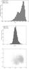Fig. 1 Distribution of the real and mock samples of redshifts z (top) and flux densities FJy at 1.4 GHz (middle). In the bottom panel, flux density vs. redshift for sources with both measurements available (Taylor et al. 2009; Hammond et al. 2012).

The positions of the sources on the sky were kept the same as for the real sources. The majority (≈40 000 sources) belong to the catalog of Taylor et al. (2009) and, for 4003 of these sources, spectroscopic redshift measurements were published by Hammond et al. (2012). For most of the sources, these catalogs give a flux density measurement that allows us to compute the luminosity of the source. Where available, we use the measured redshift and flux density. For the vast majority of the sources we generate a mock redshift and, for a few of them, we generate a mock flux density value. Mock redshifts and flux densities are extracted independently from the two observed distributions. In Fig. 1, the distribution of both the real and mock sample of redshifts and flux densities is shown in the top and middle panel, respectively. In the bottom panel, the observed flux density versus redshift distribution is presented. These two quantities appear to be weakly correlated. For sake of simplicity, we neglected such correlation in our mock simulation, since it should not have any impact on our analysis. We assume all redshifts and luminosities to be known with negligible uncertainty.

We generate a mock Faraday depth value for all of the sources in the catalog. The observed Faraday depth values consist of a Galactic, extragalactic, and noise contribution. We considered the Galactic contribution to be given by a sample extracted from the posterior of Oppermann et al. (2015). To mimic observational uncertainties, the noise variance has been computed for each source according to Eq. (37) in Oppermann et al. (2015), where as observed uncertainty, σ_i, we use the uncertainties reported in the observational catalogs and as η_i we use the values recovered by Oppermann et al. (2015). The observational error of each measurement has been extracted from a Gaussian with this standard deviation and zero mean. Concerning the extragalactic contribution, in this test we consider the 2C scenario described in Sect. 2, namely an intrinsic and an environmental contribution, 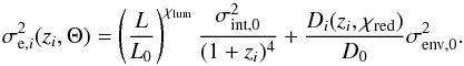${\mathit{\sigma }}_{\mathrm{e}\mathit{,i}}^{\mathrm{2}}\mathrm{\left(}{\mathit{z}}_{\mathit{i}}\mathit{,}\mathrm{\Theta }\mathrm{\right)}\mathrm{=}{\left(\frac{\mathit{L}}{{\mathit{L}}_{\mathrm{0}}}\right)}^{{\mathit{\chi }}_{\mathrm{lum}}}\frac{{\mathit{\sigma }}_{\mathrm{int}\mathit{,}\mathrm{0}}^{\mathrm{2}}}{\mathrm{(}\mathrm{1}\mathrm{+}{\mathit{z}}_{\mathit{i}}{\mathrm{)}}^{\mathrm{4}}}\mathrm{+}\frac{{\mathit{D}}_{\mathit{i}}\mathrm{\left(}{\mathit{z}}_{\mathit{i}}\mathit{,}{\mathit{\chi }}_{\mathrm{red}}\mathrm{\right)}}{{\mathit{D}}_{\mathrm{0}}}{\mathit{\sigma }}_{\mathrm{env}\mathit{,}\mathrm{0}}^{\mathrm{2}}\mathit{.}$(28)The variances in Eq. (28) depend on the redshifts and luminosities of the sources. Therefore, each source has a different variance. For each source, the extragalactic contribution is extracted from a Gaussian with this variance and zero mean. As summarized in Table  2, the contributions intrinsic to the source and due to the medium between the source and the observer are τ_σint,0 = 18.2 rad m^-2 and τ_σenv,0 = 1.4 rad m^-2, respectively. Since the mean of the factor L_i/L₀/ (1 + z_i)⁴ is ≈0.06 and the mean of the factor D_i/D₀ is ≈15.5, the standard deviation in the overall intrinsic and environmental components are ${\mathit{\sigma }}_{\mathrm{int}}^{\mathrm{true}}\mathrm{\approx }\mathrm{4.4}$ rad m^-2 and ${\mathit{\sigma }}_{\mathrm{env}}^{\mathrm{true}}\mathrm{\approx }\mathrm{5.3}$ rad m^-2. For this scenario, we run two tests corresponding to a different number of lines of sight:

• 41 632 (2C1). This is the total number of lines ofsight for which an estimate of the extragalactic contribution isavailable from Oppermann et al. (2015);

• 4003 (2C2). This number accounts for all of the sources in the catalog 2C1 for which a redshift measurement is available as well (Hammond et al. 2012).

In Fig. 2, we show the results for tests 2C1 and 2C2, meaning with a two-component scenario for 41 632 lines of sight (a) and 4003 lines of sight (b), respectively. The histograms in the top plots of each column represent the one-dimensional projection of the posterior for the corresponding parameter. The dotted lines indicate the true value of the parameter. The dashed and dash-dotted lines describe the posterior statistics, namely the mean and the 1σ confidence level, respectively. The continuous lines indicate the prior used in our analysis. The panels in colors show the two-dimensional projection of the posterior for a given couple of parameters. These plots show that our algorithm is able to recover the mock Θ values for this scenario. The inferred posterior mean values agree with the correct values within the uncertainties and the posterior distributions are much narrower than the prior distributions. The dispersion in the parameters Θ increases by decreasing the number of lines of sight, as expected. The plots indicate that some of the parameters are correlated, e.g., most noticeably σ_env,0-χ_red, which show a strong anticorrelation. This feature can be understood in light of Eq. (12). Indeed, for a given Faraday rotation σ_env associated with the structures between the source and the observer, larger σ_env,0 imply smaller χ_red and vice versa. We expect the correlation in the posterior to be significant for any reasonable parameterization that allows for the same number of degrees of freedom.

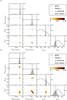Fig. 2 Results obtained with a two-component scenario for 41 632 (2C1) lines of sight in panel a) and for 4003 (2C2) in panel b). In each panel the top plots of each column show the one-dimensional projection of the posterior and the true value (dotted line), the outcome of the analysis (dashed and dash-dotted lines), and the prior (continuous line). The panels in color show the two-dimensional marginalized views of the posterior as sampled.

In order to have a compact and complete visualization, in the rest of the paper we present all of the tests we performed and their results as in Fig. 2.

3.2. Future prospects

We investigate the possibility to separate the Faraday rotation intrinsic to the emitting radio source from that due to the extragalactic environments between the source and the observer with the specifications of the SKA, its precursor, ASKAP, and its pathfinder, LOFAR. We generated the mock Faraday depth values for each source as described in Sect. 3.1. For each catalog, we extracted the noise contribution for each line of sight from a Gaussian with zero mean and standard deviation equal to maximum uncertainty in Faraday depth expected in the corresponding frequency range, according to Stepanov et al. (2008). Luminosities at frequencies different from 1.4 GHz were spectrally adjusted⁴.

Since our approach assumes that all of the lines of sight are independent, i.e., sufficiently separated (≳1°) so that the cross-correlation function of their magnetic field is zero, in the following tests we compute the number of lines of sight considering a density of sources lower than or equal to one polarized source per square degree. The expected number density of sources for ASKAP and SKA per square degree is at least 100 times larger. Here, we investigate whether already with a small sample of lines of sight we would be able to put any constraints on the contribution from extragalactic large-scale environments, rather than exploit the information delivered by the full number of lines of sight and to show the full potential of ASKAP and SKA.

3.2.1. Low-Frequency Array

We only consider the LOFAR’s high band antennas (HBA) because the calibration of the low band antennas (LBA) is very challenging owing to the ionosphere. We select the HBA region of the spectrum with less contamination from radio frequency interference (120–160 MHz; Offringa et al. 2013). In this frequency range, the uncertainty on Faraday depth values is expected to be ≤0.05 rad m^-2 for a signal-to-noise ratio larger than 5 (Stepanov et al. 2008). Ionospheric Faraday rotation can degrade the results at LOFAR frequencies; the same holds for SKA1 – band 1 observations; see the next section. Sotomayor-Beltran et al. (2013) developed an approach to model ionospheric Faraday rotations using LOFAR pulsar observations with precision up to 0.05–0.1 rad m^-2, comparable with the maximum uncertainty expected in this frequency band and considered here (see Table 1). According to Mulcahy et al. (2014), the expected number of polarized extragalactic radio sources is 1 per 1.7 square degrees for 8 h-long observations, assuming an average degree of polarization of 1%, a spatial resolution of 20′′, and a detection threshold of 500 μJy/beam/rmsf⁵ that corresponds to S/N = 5.

On the basis of these assumptions we generate coordinates in the sky for a collection of sources corresponding to a survey (8 h per pointing) in the direction of the north polar cap (NP). Among these sources we select those with Galactic latitude larger than 55°. This results in approximately 2200 sources. We derive a catalog assuming an overall extragalactic Faraday rotation σ_e ≈ 7 rad m^-2 (NPa), and one assuming an overall extragalactic Faraday rotation σ_e ≈ 0.7 rad m^-2 (NPb). The results are shown in Fig. 3, panels a and b. These plots show that LOFAR can provide good constraints for both values of the overall extragalactic Faraday depth if a few thousand of lines of sight are used with better performance for larger σ_e. The posterior distributions are much narrower than the prior distributions and the posterior means agree with the correct values within 1–2σ. We also performed tests with a smaller number of lines of sight (N_los ≈ 1000, see Tables 1, 2, and Fig. 6) still obtaining good performances even if, as expected, the posterior distributions were wider.

A survey of the sky at similar frequencies (170–200 MHz) but with lower spatial resolution (15.6′) was conducted with the Murchison Widefield Array over an area of 2400 deg² (Bernardi et al. 2013). With a sensitivity in total intensity of 200 mJy/beam, the authors detected polarized emission only for one source among all of the sources brighter than 4 Jy, implying at these frequencies a fractional polarization below 2% for the remaining sources. The low number density derived by Bernardi et al. (2013) may be due to beam depolarization. The number of polarized sources in this frequency band is not yet clear and different assumptions on the density of sources translate to different predictions on the capabilities to infer properties of extragalactic magnetic fields.

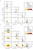Fig. 3 As Fig. 2 but for results obtained with a two-component scenario for LOFAR HBA observations for Nlos ≈ 2200 and an overall extragalactic standard deviation in Faraday depth of a) ≈7 rad m-2 (NPa) and b) ≈0.7 rad m-2 (NPb).

Fig. 4 As Fig. 2 but for results obtained with a two-component scenario for SKA observations in the frequency range 650–1670 MHz for Nlos ≈ 3500 and an overall extragalactic Faraday rotation of a) ≈7.0 rad m-2 (B2SP1a) and b) ≈0.7 rad m-2 (B2SP1b).

We note that at frequencies ≈GHz the Galactic contribution can be described with a single Faraday screen along the line of sight (i.e., Uyaniker & Landecker 2002; Wolleben & Reich 2004). In the frequency band of LOFAR, the Galactic contribution can become more complex (e.g., Bernardi et al. 2009; Jelić et al. 2014; Zaroubi et al. 2015) with multiple, statistically significant Faraday depth peaks for several lines of sight. The tests performed here assume the simple scenario of a single-component Faraday depth spectrum. A more realistic treatment would require a more complex model for the Galactic foreground and is left for future work.

3.2.2. Square Kilometre Array

The SKA is expected to observe the entire Southern sky with a spatial resolution of 2′′ and a sensitivity in polarization of ≈4 μJy/beam (see, e.g., Johnston-Hollitt et al. 2015). The resulting sky grid of Faraday rotation values will be 200–300 times denser than the largest catalog currently available (see, e.g., Hales 2013). The better resolution of 2′′, compared to the 45′′ of Taylor et al. (2009), will make it possible to identify optical counterparts uniquely and, hence, to assign a redshift estimate to a larger number of sources through spectroscopic follow-up observations. The SKA1 Re-Baseline Design 2015 indicates the frequency bands 1, 2, and 5 as available on SKA_MID during SKA-Phase 1:

• band 1, 0.35–1.05 GHz;

• band 2, 0.95–1.76 GHz;

• band 5, 4.6–13.8 GHz.

In the following we consider the frequency range 0.95–1.76 GHz, since receivers in band 2 (B2SP1) should be constructed first.

We produce mock Faraday depth values assuming a maximum standard deviation in the noise distribution of the Faraday depth of 2.0 rad m^-2, according to Stepanov et al. (2008), for this frequency range and for S/N > 5. We generate a catalog of coordinates in the south polar cap (SP) based on the assumption of one polarized source per square degree and we select those with Galactic latitude b < −55°. This translates in N_los ≈ 3500. We refer to this catalog as B2SP1. We produce catalogs of Faraday depth values assuming σ_e ≈ 7.0 rad m^-2 (B2SP1a) and σ_e ≈ 0.7 rad m^-2 (B2SP1b).

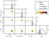Fig. 5 As Fig. 2 but for results obtained with a two-component scenario for ASKAP observations in the frequency range 1130–1430 MHz for Nlos ≈ 3500 and an overall Faraday depth of ≈7.0 rad m-2 (POS).

In Fig. 4, we show the results for B2SP1a and B2SP1b, in panels a and b, respectively. The plots for σ_e ≈ 7.0 rad m^-2 indicate that with N_los ≈ 3500 we obtain a good disentangling of the environmental and intrinsic contributions and their redshift and luminosity dependence with narrow posterior distributions and mean values within ≈1σ from the true values. For the same amount of lines of sight but a smaller overall Faraday rotation σ_e ≈ 0.7 rad m^-2, the dispersion in σ_int,0, χ_lum, and χ_red becomes broader but with mean values still within a few standard deviations from the assumed value. On the other hand, we do not get good constraints for the parameter σ_env,0 that appears to be characterized by a large dispersion. The posterior distributions are much broader than those derived with LOFAR for the same overall extragalactic Faraday rotation (see Fig. 3). This is because of the different frequency range considered here. Indeed, despite the larger number of lines of sight included in this catalog, the maximum uncertainty in Faraday depth is larger by one order of magnitude, preventing the algorithm from constraining the Θ parameters with high precision. In order to derive narrower posterior distributions, we would need to resort to a larger number of lines of sight or to a smaller observational uncertainty in Faraday depth. Since the sensitivity of the SKA will allow us to detect hundreds of sources per square degree, narrower posterior distribution of the parameters can be obtained by increasing the number of lines of sight.

For an overall extragalactic contribution σ_e ≈ 7 rad m^-2, further tests with a smaller number of lines of sight (N_los ≈ 1000) show good performances, even if the posterior distributions are broader. In addition, for a direct comparison with LOFAR, we run tests for SKA observations in band 1 and obtain consistent results. All these tests are summarized in Table 2 and Fig. 6. In this paper, we do not consider the SKA frequency band 5. Even if by moving to a higher frequency sources have a higher degree of polarization, the maximum uncertainty in Faraday depth is larger and the total source counts is reduced. Consequently, we expect that the parameters are poorly constrained if the same number of lines of sight is taken.

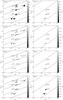Fig. 6 Uncertainty on σint,0, σenv,0, χlum, and χred (from the top to the bottom) as a function of the observational uncertainty σnoise and the number of lines of sight Nlos for an overall extragalactic Faraday depth variance of ≈7.0 rad m-2 (left panels) and ≈0.7 rad m-2 (right panels). The size of the points is proportional to the uncertainty on the parameter. A description of this uncertainty is given also by the grayscale. Circles refer to scenarios including two components, while triangles refer to three-component scenarios. Continuous lines correspond to ${\mathit{\sigma }}_{\mathrm{noise}}^{\mathrm{2}}\mathit{/}{\mathit{N}}_{\mathrm{los}}$ = const.

The high spatial resolution of the polarization survey planned with SKA1, 2′′, will permit us to resolve the large majority of the sources and, consequently, to image Faraday depth spatial variations on scales smaller than the source size. Therefore, we will be able to access the spatial correlation of the Faraday depth intrinsic to the source and of that due to the screen in front of it. The current version of the algorithm does not take into account any correlation of the magnetic field along different lines of sight. Therefore, its application to such a dense Faraday depth catalog would deliver a lower limit on the magnetic field strength, including only the uncorrelated component.

3.2.3. Australian Square Kilometre Array Pathfinder

The Polarisation Sky Survey of the Universe’s Magnetism (POSSUM; Gaensler et al. 2010) is planned between 1130 and 1430 MHz with ASKAP. The survey will reach a sensitivity in U and Q of <10 μJy/beam and a resolution of 10′′. This will result in a density of 70 polarized sources per square degree (Hales et al. 2014) and a Faraday depth catalog that is 100 times denser than those that currently exist (e.g., Taylor et al. 2009). To test the capabilities of this survey in constraining extragalactic magnetic fields, we use the same setup described in Sect. 3.2.2, but with an uncertainty drawn from a Gaussian with σ_noise = 6.0 rad m^-2. This should be a reliable approximation of the maximum uncertainty in Faraday depth for a polarized signal with a S/N > 5 (Stepanov et al. 2008). The results are shown in Fig. 5. ASKAP observations already appear very promising for disentangling the contribution intrinsic to the source from that due to large-scale environments for σ_e ≈ 7.0 rad m^-2; this is already the case if Faraday depth values are only available for one source per square degree. The dispersion in the parameters is larger than that derived in Sect. 3.2.2 for the same collection of sources and overall extragalactic Faraday variance (Fig. 4a), as expected as the maximum uncertainty in Faraday depth is larger. However, the mean values of the posterior agree with the true values within at most about 1σ.

3.3. Discussion

We developed a Bayesian algorithm to disentangle extragalactic contributions in the Faraday depth signal. This algorithm builds upon an algorithm to reconstruct the Galactic Faraday screen and its uncertainty-correlation structure previously presented by Oppermann et al. (2015). We tested the algorithm by modeling the overall extragalactic contribution as the sum of an intrinsic and an environmental component; as described in Sect. 3.1, but see Appendix C for the inclusion of a constant or a latitude-dependent term. These tests show that the algorithm is able to discriminate among the different components and their dependence on the luminosity and redshift of the source.

For test purposes, we built mock catalogs according to the specifications of the catalogs available in the literature after correcting for poorly known uncertainty information (see Sect. 3.1). The results in Fig. 2b indicate that by applying the algorithm to the currently available dataset, we could already infer preliminary information about extragalactic magnetic fields if a few thousand sources with reliable observational uncertainty were available. For the 4003 sources in Fig. 2b, indeed, redshift and flux density values are available. Nevertheless, since actually we do not consider all their Faraday depth noise variances to be reliable (see Appendix A of Oppermann et al. 2015) and the applied correction factors, η_i, are only statistical estimates, we would need to sample in the η_i-parameter space as well to use the algorithm with real data, as described by Oppermann et al. (2015).

The modern techniques of analysis, such as model fitting of the fractional polarization components q and u (e.g., Farnsworth et al. 2011; Ideguchi et al. 2014), rotation measure synthesis (e.g., Brentjens & de Bruyn 2005; Akahori et al. 2014b) and Faraday synthesis (Bell & Enßlin 2012), and the future radio surveys will partially overcome this problem. The large bandwidth of the new radio interferometers will allow us to reduce the risk of nπ-ambiguity, which is particularly strong when the λ²-fit approach is used, as well as to reach a sufficiently high resolution in Faraday depth to distinguish nearby Faraday components. We note that when the distance between two peaks in a Faraday spectrum is smaller than the resolution, the uncertainty in the Faraday depth may be driven by the Faraday point spread function (e.g., Farnsworth et al. 2011; Farnes et al. 2014b; Kumazaki et al. 2014). For these reasons, the catalogs coming from Faraday depth grids planned with LOFAR, ASKAP, and the SKA will be more reliable both in terms of Faraday depth values and uncertainties.

Therefore, we investigate the prospects of these simpler future datasets here and address the more complex application of our technique to present data in a separate work. We assumed the computation to be dominated by the uncertainties in the Faraday depth estimates for each source, while the coordinates, luminosities, and redshifts to be exactly known. With the advent of highly-accurate Faraday depth catalogs, this may change and in future work we will need to investigate to what depths and accuracy redshifts, and luminosities are needed to apply the method we propose. This is particularly important for redshifts. Indeed, the catalog used in this work reports a spectroscopic redshift for each source (Hammond et al. 2012). Recently, optical surveys, such as 2MASS, WISE, and SuperCOSMOS have measured the photometric redshifts for millions of galaxies up to z ≈ 0.5 (e.g., Bilicki et al. 2014), and the surveys planned with the next generation of telescopes will further increment this number. Nevertheless, photometric redshifts are less accurate than spectroscopic redshifts. This will require us to evaluate the impact of their uncertainties on our results.

Our tests indicate that LOFAR, ASKAP, and the SKA will allow us to infer information about cosmological magnetic fields already with a few thousands of lines of sight with better performance when lower frequencies are used. We want to stress that the uncertainties used in our tests only represent statistical uncertainties and any systematic issues have been neglected. In principle, LOFAR observations could already be used for this aim but the development of a pipeline for the reduction of polarization data is still in progress. The enhanced capabilities of the Jansky Very Large Array (JVLA) make the new centimeter-wavelength sky survey (VLASS⁶) planned with this instrument a good opportunity for the application of this algorithm and for delivering significant results in the study of cosmic magnetism in the near future. Similarly, the frequency range (1–1.75 GHz), the angular resolution (13′′), the expected sensitivity (10 μJy/beam over 300 MHz of bandwidth and 12 hours of observation), and the large field of view (8 square degrees) make the APERture Tile In Focus (APERTIF⁷) a competitive instrument for the present investigation of cosmological magnetic fields.

In Table 2 we give a quantitative summary of the results. For each test we report the true values τ of the Θ parameters that describe the intrinsic and environmental contribution to the Faraday depth, their mean values μ, their uncertainties σ, and the displacement of the mean from the true value in terms of the uncertainty, $\mathit{ϵ}\mathrm{=}\left|\frac{\mathit{\mu }\mathrm{-}\mathit{\tau }}{\mathit{\sigma }}\right|\mathrm{·}$(29)These values were computed after discarding the burn-in samples by visual inspection. The comparison of the results obtained with the mock catalogs created for present instruments 2C1 and 2C2 indicates that by increasing the number of sources with known redshift by a factor ten, the uncertainty in the Θ parameters can be reduced by about a factor two. This would not longer be valid if the sources without redshift information represent a different population than the observed population, since in our test we adopted mock values for these sources randomly extracted from the observed redshift distribution. A similar result is obtained if the observational uncertainty σ_noise is reduced by approximately a factor ten, as shown by the comparison of results corresponding to catalog 2C2 and the SKA catalog B2SP1a. These two tests refer to a similar number of lines of sight and to a similar mean frequency⁸. In Fig. 6 we present a visual summary of the results for all of the two- and three-component scenarios corresponding to an overall extragalactic Faraday rotation of approximately both 7 rad m^-2 (left panels) and 0.7 rad m^-2 (right panels) for the four parameters σ_int,0, σ_env,0, χ_lum, and χ_red. The uncertainty on the parameters Θ decreases by increasing the number of lines of sight, N_los, and by decreasing the observational error, σ_noise. The best results are obtained when a good compromise between these two numbers is used, as for example shown by the scenarios B1SP1a and B1SP1b. Nevertheless, the comparison of the results of tests corresponding to different instruments can be not straightforward because they refer to different frequency bands and to slightly different values of the Θ parameters.

The problem we are tackling is characterized by different complexities. We are looking for a very weak signal by using the residual information left in the data after the Galactic contribution is derived. At the same time, we expect this signal to be characterized by a possible redshift dependence, even if this dependence is very weak since it is not yet detected, and by cross-correlations of the extragalactic magnetic field along different lines of sight. In this work, we try to address the first two issues with a Bayesian approach that is able to combine all of the available observational information properly and allow for a redshift dependence in our model. On the one hand, we might overestimate the extragalactic contributions, since we are not including an uncorrelated Galactic component in the model. This term can be easily included in our algorithm, as shown by the tests in Appendix C and quantified with real data. On the other hand, we do not take into account a possible correlated component of the extragalactic magnetic field, which if present would be beneficial for our analysis. This means that the magnetic field values that can be inferred have to be considered rather as a lower limit, even if we expect this error to be small (e.g., Akahori & Ryu 2011). This is not a problem for surveys performed with LOFAR, since the expected density of extragalactic polarized sources is lower than one source per square degree. On the contrary, with ASKAP and the SKA, we will be able to detect at least 100 sources per square degree. An approach to deal with possible cross-correlations between lines of sight is being developed with the intention to apply this new technique to forthcoming ultradeep JVLA observations from the CHILES Con Pol survey (Hales et al., in prep.). The combination of the two methods would allow us to exploit in an optimal way the information coming from the denser grids of Faraday depth measurements provided by SKA and ASKAP surveys.

Finally, we stress that the aim of this paper is to give a proof of concept. Indeed, the present version of the algorithm requires a high computational burden that limits its efficiency. For example, the time required to run a test on our computer cluster is on the order of a couple of months per chain even when only a few thousands lines of sight are considered. We are currently working on performance optimization to make the algorithm suitable to be applied to the upcoming large Faraday depth catalogs.

3.4. Future developments

The work presented in this paper prepares a Bayesian technique to investigate magnetic fields in the large-scale structure, in particular, in filaments and voids. As a next step, we want to discriminate among the amount of Faraday rotation due to each large-scale structure environment (see also Vacca et al. 2015). When different large-scale environments are considered, the variance in the extragalactic Faraday rotation can be parameterized as $\begin{array}{ccc}\mathrm{⟨}{\mathit{\phi }}_{\mathrm{e}\mathit{,i}}^{\mathrm{2}}\mathrm{⟩}& \mathrm{\approx }& {\mathit{a}}_{\mathrm{0}}^{\mathrm{2}}{\mathrm{\int }}_{\mathrm{0}}^{{\mathit{z}}_{\mathit{i}}}\mathrm{⟨}{\mathit{n}}_{\mathrm{0}}^{\mathrm{2}}\mathrm{⟩}\mathrm{⟨}{\mathit{B}}_{\mathit{l}\mathrm{0}}^{\mathrm{2}}\mathrm{⟩}{\mathrm{\Lambda }}_{\mathit{l}\mathrm{0}}\mathrm{(}\mathrm{1}\mathrm{+}\mathit{z}{\mathrm{)}}^{\mathrm{4}}\frac{\mathit{c}}{\mathit{H}\mathrm{\left(}\mathit{z}\mathrm{\right)}}\mathrm{d}\mathit{z}\\ & \mathrm{\approx }& \end{array}$(30)where σ₁,σ₂,...,σ_Nenv are the contributions from N_env different environments and l_ij is the length of the line of sight, i, through each environment, j.

With a Bayesian approach, Jasche et al. (2010) (see also Leclercq et al. 2015) reconstructed the cosmic density field. They used optical data from the Sloan Digital Sky Survey (SDSS) Data Release 7 (Abazajian et al. 2009) and classified the structures as voids, sheets, filaments, and galaxy clusters, according to the classification scheme of Hahn et al. (2007). This reconstruction enables us to compute the path covered by the radio signal through each environment, i.e., the elements l_ij in Eq. (30), once the position of the radio source is identified using the redshift. This posterior of the large-scale structure density field is available in the form of samples. Radio sources can belong to different environments (e.g., galaxy clusters and filaments) and the path covered by the signal in each environment differs for each radio source. These facts can be statistically taken into account with the use of a collection of sources distributed over all of the sky and of different realizations of the large-scale structure. We plan to use the full posterior of the large-scale structure to statistically estimate the amount of variance due to the different types of environments in the observed Faraday depths.

4. Conclusions

The properties of cosmic magnetic fields constitute outstanding questions in modern cosmology. To get a better understanding, it is essential to shed light on the properties of magnetic fields in large-scale environments, meaning filaments and voids, where turbulent intracluster gas motions have not yet enhanced the magnetic field and, consequently, the magnetic field strength and structure still depend on the seed field power spectrum.

Upcoming generations of radio telescopes, first LOFAR, and in the next decades the SKA, will perform polarization sky surveys with high sensitivity. Modern techniques based on rotation measure synthesis and Faraday synthesis, will enable us to perform a proper analysis of the polarization properties of extragalactic radio sources, thus providing unprecedented, highly accurate Faraday depth catalogs in frequency ranges from a few hundreds MHz to a few GHz. A statistical approach is required to exploit the information encoded in these data. For this reason, we developed a Bayesian algorithm that is able to combine radio observations with luminosities and redshifts of sources, aiming at disentangling contributions to the extragalactic Faraday rotation intrinsic to radio sources and due to large-scale structures, and in this way infer information about large-scale magnetic fields. Knowledge of the redshift is essential in this approach. The present all-sky photometric optical surveys and the surveys planned with the next generation of telescopes will greatly enlarge the number of sources for which this information will be available.

The work described in this paper is a proof of concept and shows that our algorithm can be used to discriminate between the Faraday depth generated by the radio source itself and the contribution due to large-scale structures. Additionally, our algorithm is able to investigate the dependence of these terms on the redshift and radio luminosity of the sources. The tests performed with mock LOFAR, ASKAP, and SKA data suggest that this technique is promising for the investigation of magnetic fields with strengths of a few μG down to a few nG, when uncertainties in the data are up to a few rad m^-2 and known with high accuracy. Our modeling does not take into account any correlated component of extragalactic magnetic fields. Consequently, inferred magnetic field strengths have to be considered as a lower limit.

The main characteristics of upcoming polarization surveys can be summarized by the number of lines of sight and by the maximum observational uncertainty in Faraday depth. Our tests indicate that, for a given number of lines of sight, better constraints can be obtained with observations at lower frequencies because of the smaller observational uncertainty. Therefore, in principle, LOFAR observations and, even more so, SKA_LOW (50–350 MHz) observations, thanks to their higher sensitivity, would be ideal. Nevertheless, the scant number of polarized sources at these frequencies and the difficulties in the calibration of the data could make the use of these data complex. Observations by ASKAP and SKA_MID in the frequency range 1130–1430 MHz and 650–1670 MHz, respectively, appear to be promising as well. We should be able to put useful constraints on large-scale magnetic fields already with Faraday depth measurements for a few thousands of sources, and improve their determination by increasing the number of lines of sight. An increment in the number of lines of sight by a given factor reduces the uncertainty in the estimation of the intrinsic and environmental contribution as a reduction by approximately the same factor in the observational uncertainty does, indicating that deeper observations of small fields could be a valuable or even better alternative to all sky surveys.

We are aware that many aspects of our approach require improvements, for example, computational efficiency, inclusion of a correlated extragalactic magnetic field component, and of uncertainty in redshift. Nevertheless, we present a first step toward a Bayesian study of magnetic fields associated with the cosmic large-scale structures.

Acknowledgments

We thank the anonymous referee for useful comments and suggestions. V.V. thanks Federica Govoni, Mark Birkinshaw, Matteo Murgia, Anna Scaife, and Gabriele Giovannini for useful discussions. The implementation of the code makes use of the NIFTY package by Selig et al. (2013) and of the cosmology calculator by Ned Wright (www.astro.ucla.edu/~wright). This research was supported by the DFG Forschengruppe 1254 “Magnetisation of Interstellar and Intergalactic Media: The Prospects of Low-Frequency Radio Observations”. K.T. is supported by Grant-in-Aid from the Ministry of Education, Culture, Sports, Science and Technology (MEXT) of Japan, Nos. 24340048 and 26610048. T.S. and H.R. acknowledge support from the ERC Advanced Investigator programme NewClusters 321271.

References

Appendix A: Extragalactic Faraday depth variance

In this Appendix, we derive Eq. (9) from Eq. (5). In Eq. (5) we define the extragalactic Faraday depth variance as $\mathrm{⟨}{\mathit{\phi }}_{\mathrm{e}\mathit{,i}}^{\mathrm{2}}\mathrm{⟩}\mathrm{\approx }{\mathit{a}}_{\mathrm{0}}^{\mathrm{2}}{\mathrm{\int }}_{\mathrm{0}}^{{\mathit{z}}_{\mathit{i}}}\frac{\mathrm{d}\mathit{l}}{\mathrm{d}\mathit{z}}{\mathrm{\int }}_{\mathrm{0}}^{{\mathit{z}}_{\mathit{i}}}\frac{\mathrm{d}{\mathit{l}}^{\mathrm{\prime }}}{\mathrm{d}{\mathit{z}}^{\mathrm{\prime }}}\mathrm{⟨}{\mathit{n}}_{\mathrm{e}}\mathrm{\left(}\mathit{z}\mathrm{\right)}{\mathit{n}}_{\mathrm{e}}\mathrm{\left(}{\mathit{z}}^{\mathrm{\prime }}\mathrm{\right)}{\mathit{B}}_{\mathit{l}}\mathrm{\left(}\mathit{z}\mathrm{\right)}{\mathit{B}}_{\mathit{l}}\mathrm{\left(}{\mathit{z}}^{\mathrm{\prime }}\mathrm{\right)}\mathrm{⟩}\mathrm{d}\mathit{z}\mathrm{d}{\mathit{z}}^{\mathrm{\prime }}\mathit{.}$(A.1)This definition can also be expressed as a function of distance along the line of sight l$\mathrm{⟨}{\mathit{\phi }}_{\mathrm{e}\mathit{,i}}^{\mathrm{2}}\mathrm{⟩}\mathrm{\approx }{\mathit{a}}_{\mathrm{0}}^{\mathrm{2}}{\mathrm{\int }}_{\mathrm{0}}^{\mathit{l}\mathrm{\left(}{\mathit{z}}_{\mathit{i}}\mathrm{\right)}}\mathrm{d}\mathit{l}{\mathrm{\int }}_{\mathrm{0}}^{\mathit{l}\mathrm{\left(}{\mathit{z}}_{\mathit{i}}\mathrm{\right)}}\mathrm{d}{\mathit{l}}^{\mathrm{\prime }}\mathrm{⟨}{\mathit{n}}_{\mathrm{e}}\mathrm{\left(}\mathit{l}\mathrm{\right)}{\mathit{n}}_{\mathrm{e}}\mathrm{\left(}{\mathit{l}}^{\mathrm{\prime }}\mathrm{\right)}{\mathit{B}}_{\mathit{l}}\mathrm{\left(}\mathit{l}\mathrm{\right)}{\mathit{B}}_{\mathit{l}}\mathrm{\left(}{\mathit{l}}^{\mathrm{\prime }}\mathrm{\right)}\mathrm{⟩}\mathit{.}$(A.2)If we assume that the thermal gas density is not characterized by significant fluctuations and define a new variable r = l′−l, we have 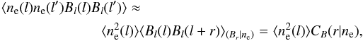$\begin{array}{ccc}\mathrm{⟨}{\mathit{n}}_{\mathrm{e}}\mathrm{\left(}\mathit{l}\mathrm{\right)}{\mathit{n}}_{\mathrm{e}}\mathrm{\left(}{\mathit{l}}^{\mathrm{\prime }}\mathrm{\right)}{\mathit{B}}_{\mathit{l}}\mathrm{\left(}\mathit{l}\mathrm{\right)}{\mathit{B}}_{\mathit{l}}\mathrm{\left(}{\mathit{l}}^{\mathrm{\prime }}\mathrm{\right)}\mathrm{⟩}& \mathrm{\approx }& \\ & & \mathrm{⟨}{\mathit{n}}_{\mathrm{e}}^{\mathrm{2}}\mathrm{\left(}\mathit{l}\mathrm{\right)}\mathrm{⟩}\mathrm{⟨}{\mathit{B}}_{\mathit{l}}\mathrm{\left(}\mathit{l}\mathrm{\right)}{\mathit{B}}_{\mathit{l}}\mathrm{(}\mathit{l}\mathrm{+}\mathit{r}\mathrm{)}{\mathrm{⟩}}_{\mathrm{\left(}{\mathit{B}}_{\mathit{r}}\mathrm{\right|}{\mathit{n}}_{\mathrm{e}}\mathrm{)}}\mathrm{=}\mathrm{⟨}{\mathit{n}}_{\mathrm{e}}^{\mathrm{2}}\mathrm{\left(}\mathit{l}\mathrm{\right)}\mathrm{⟩}{\mathit{C}}_{\mathit{B}}\mathrm{\left(}\mathit{r}\mathrm{\right|}{\mathit{n}}_{\mathrm{e}}\mathrm{)}\mathit{,}\end{array}$(A.3)where C_B(r | n_e) is the conditional magnetic field correlation function for an environment with thermal gas density n_e. Indeed, we expect the magnetic field strength to be a function of the thermal gas density. With these new definitions, the extragalactic Faraday depth variance reads 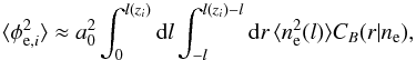$\mathrm{⟨}{\mathit{\phi }}_{\mathrm{e}\mathit{,i}}^{\mathrm{2}}\mathrm{⟩}\mathrm{\approx }{\mathit{a}}_{\mathrm{0}}^{\mathrm{2}}{\mathrm{\int }}_{\mathrm{0}}^{\mathit{l}\mathrm{\left(}{\mathit{z}}_{\mathit{i}}\mathrm{\right)}}\mathrm{d}\mathit{l}{\mathrm{\int }}_{\mathrm{-}\mathit{l}}^{\mathit{l}\mathrm{\left(}{\mathit{z}}_{\mathit{i}}\mathrm{\right)}\mathrm{-}\mathit{l}}\mathrm{d}\mathit{r}\hspace{0.17em}\mathrm{⟨}{\mathit{n}}_{\mathrm{e}}^{\mathrm{2}}\mathrm{\left(}\mathit{l}\mathrm{\right)}\mathrm{⟩}{\mathit{C}}_{\mathit{B}}\mathrm{\left(}\mathit{r}\mathrm{\right|}{\mathit{n}}_{\mathrm{e}}\mathrm{)}\mathit{,}$(A.4)which can be further simplified if we consider the limit of an infinitely far away source, 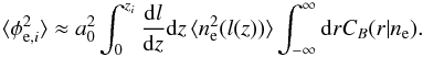$\mathrm{⟨}{\mathit{\phi }}_{\mathrm{e}\mathit{,i}}^{\mathrm{2}}\mathrm{⟩}\mathrm{\approx }{\mathit{a}}_{\mathrm{0}}^{\mathrm{2}}{\mathrm{\int }}_{\mathrm{0}}^{{\mathit{z}}_{\mathit{i}}}\frac{\mathrm{d}\mathit{l}}{\mathrm{d}\mathit{z}}\mathrm{d}\mathit{z}\hspace{0.17em}\mathrm{⟨}{\mathit{n}}_{\mathrm{e}}^{\mathrm{2}}\mathrm{\left(}\mathit{l}\mathrm{\right(}\mathit{z}\mathrm{\left)}\mathrm{\right)}\mathrm{⟩}{\mathrm{\int }}_{\mathrm{-}\mathrm{\infty }}^{\mathrm{\infty }}\mathrm{d}\mathit{r}{\mathit{C}}_{\mathit{B}}\mathrm{\left(}\mathit{r}\mathrm{\right|}{\mathit{n}}_{\mathrm{e}}\mathrm{)}\mathit{.}$(A.5)Recalling the definition of correlation length, 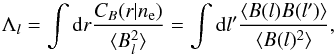${\mathrm{\Lambda }}_{\mathit{l}}\mathrm{=}\mathrm{\int }\mathrm{d}\mathit{r}\frac{{\mathit{C}}_{\mathit{B}}\mathrm{\left(}\mathit{r}\mathrm{\right|}{\mathit{n}}_{\mathrm{e}}\mathrm{)}}{\mathrm{⟨}{\mathit{B}}_{\mathit{l}}^{\mathrm{2}}\mathrm{⟩}}\mathrm{=}\mathrm{\int }\mathrm{d}{\mathit{l}}^{\mathrm{\prime }}\frac{\mathrm{⟨}\mathit{B}\mathrm{\left(}\mathit{l}\mathrm{\right)}\mathit{B}\mathrm{\left(}{\mathit{l}}^{\mathrm{\prime }}\mathrm{\right)}\mathrm{⟩}}{\mathrm{⟨}\mathit{B}\mathrm{(}\mathit{l}{\mathrm{)}}^{\mathrm{2}}\mathrm{⟩}}\mathit{,}$(A.6)we obtain 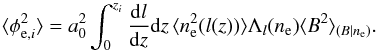$\mathrm{⟨}{\mathit{\phi }}_{\mathrm{e}\mathit{,i}}^{\mathrm{2}}\mathrm{⟩}\mathrm{=}{\mathit{a}}_{\mathrm{0}}^{\mathrm{2}}{\mathrm{\int }}_{\mathrm{0}}^{{\mathit{z}}_{\mathit{i}}}\frac{\mathrm{d}\mathit{l}}{\mathrm{d}\mathit{z}}\mathrm{d}\mathit{z}\hspace{0.17em}\mathrm{⟨}{\mathit{n}}_{\mathrm{e}}^{\mathrm{2}}\mathrm{\left(}\mathit{l}\mathrm{\right(}\mathit{z}\mathrm{\left)}\mathrm{\right)}\mathrm{⟩}{\mathrm{\Lambda }}_{\mathit{l}}\mathrm{\left(}{\mathit{n}}_{\mathrm{e}}\mathrm{\right)}\mathrm{⟨}{\mathit{B}}^{\mathrm{2}}{\mathrm{⟩}}_{\mathrm{\left(}\mathit{B}\mathrm{\right|}{\mathit{n}}_{\mathrm{e}}\mathrm{)}}\mathit{.}$(A.7)As described in Sect. 2, in a homogeneous Universe n_e = n_e0(1 + z)³, Λ_l = Λ_l0(1 + z)^-1, and $\mathrm{⟨}{\mathit{B}}^{\mathrm{2}}\mathrm{⟩}\mathrm{=}\mathrm{⟨}{\mathit{B}}_{\mathrm{0}}^{\mathrm{2}}\mathrm{⟩}\mathrm{(}\mathrm{1}\mathrm{+}\mathit{z}{\mathrm{)}}^{\mathrm{4}}$. Therefore, 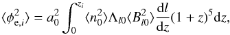$\mathrm{⟨}{\mathit{\phi }}_{\mathrm{e}\mathit{,i}}^{\mathrm{2}}\mathrm{⟩}\mathrm{=}{\mathit{a}}_{\mathrm{0}}^{\mathrm{2}}{\mathrm{\int }}_{\mathrm{0}}^{{\mathit{z}}_{\mathit{i}}}\mathrm{⟨}{\mathit{n}}_{\mathrm{0}}^{\mathrm{2}}\mathrm{⟩}{\mathrm{\Lambda }}_{\mathit{l}\mathrm{0}}\mathrm{⟨}{\mathit{B}}_{\mathit{l}\mathrm{0}}^{\mathrm{2}}\mathrm{⟩}\frac{\mathrm{d}\mathit{l}}{\mathrm{d}\mathit{z}}\mathrm{(}\mathrm{1}\mathrm{+}\mathit{z}{\mathrm{)}}^{\mathrm{5}}\mathrm{d}\mathit{z,}$(A.8)where the increment in wavelength due to the expansion of the Universe has been taken into account as well and we have assumed z(l) ≈ z(l + r). If we use the definition of proper displacement along a light ray dl/ dz = c(1 + z)^-1/H(z), this finally leads to Eq. (9), 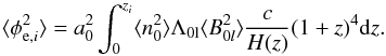$\mathrm{⟨}{\mathit{\phi }}_{\mathrm{e}\mathit{,i}}^{\mathrm{2}}\mathrm{⟩}\mathrm{=}{\mathit{a}}_{\mathrm{0}}^{\mathrm{2}}{\mathrm{\int }}_{\mathrm{0}}^{{\mathit{z}}_{\mathit{i}}}\mathrm{⟨}{\mathit{n}}_{\mathrm{0}}^{\mathrm{2}}\mathrm{⟩}{\mathrm{\Lambda }}_{\mathrm{0}\mathrm{l}}\mathrm{⟨}{\mathit{B}}_{\mathrm{0}\mathit{l}}^{\mathrm{2}}\mathrm{⟩}\frac{\mathit{c}}{\mathit{H}\mathrm{\left(}\mathit{z}\mathrm{\right)}}\mathrm{(}\mathrm{1}\mathrm{+}\mathit{z}{\mathrm{)}}^{\mathrm{4}}\mathrm{d}\mathit{z}\mathit{.}$(A.9)In an inhomogeneous Universe with different environments, the differential variance in each environment is 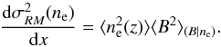$\frac{\mathrm{d}{\mathit{\sigma }}_{\mathit{RM}}^{\mathrm{2}}\mathrm{\left(}{\mathit{n}}_{\mathrm{e}}\mathrm{\right)}}{\mathrm{d}\mathit{x}}\mathrm{=}\mathrm{⟨}{\mathit{n}}_{\mathrm{e}}^{\mathrm{2}}\mathrm{\left(}\mathit{z}\mathrm{\right)}\mathrm{⟩}\mathrm{⟨}{\mathit{B}}^{\mathrm{2}}{\mathrm{⟩}}_{\mathrm{\left(}\mathit{B}\mathrm{\right|}{\mathit{n}}_{\mathrm{e}}\mathrm{)}}\mathit{.}$(A.10)Therefore, it follows 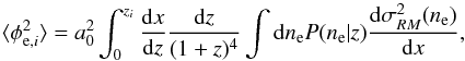$\mathrm{⟨}{\mathit{\phi }}_{\mathrm{e}\mathit{,i}}^{\mathrm{2}}\mathrm{⟩}\mathrm{=}{\mathit{a}}_{\mathrm{0}}^{\mathrm{2}}{\mathrm{\int }}_{\mathrm{0}}^{{\mathit{z}}_{\mathit{i}}}\frac{\mathrm{d}\mathit{x}}{\mathrm{d}\mathit{z}}\frac{\mathrm{d}\mathit{z}}{\mathrm{(}\mathrm{1}\mathrm{+}\mathit{z}{\mathrm{)}}^{\mathrm{4}}}\mathrm{\int }\mathrm{d}{\mathit{n}}_{\mathrm{e}}\mathit{P}\mathrm{\left(}{\mathit{n}}_{\mathrm{e}}\mathrm{\right|}\mathit{z}\mathrm{)}\frac{\mathrm{d}{\mathit{\sigma }}_{\mathit{RM}}^{\mathrm{2}}\mathrm{\left(}{\mathit{n}}_{\mathrm{e}}\mathrm{\right)}}{\mathrm{d}\mathit{x}}\mathit{,}$(A.11)where the integral can be replaced by a discrete sum over typical environments (see also Eq. (30)).

Appendix B: Convergence

We start the algorithm from two random positions in the Θ space and then explore the space⁹ until convergence. Each of these two sequences of steps in the Θ space is called Gibbs chain. To assess convergence of each Gibbs chain, we require the following conditions to be satisfied:

• the number of steps taken from each chain to be at least about10l_c for each parameter, where l_c is the number of steps at which the correlation coefficient ρ_j drops to 10%;

• the Gelman and Rubin test (Gelman & Rubin 1992; Brooks & Gelman 1997). We evaluate the intrachain variance $\mathit{I}\mathrm{=}\frac{\mathrm{1}}{\mathit{m}}{\mathrm{\Sigma }}_{\mathit{j}\mathrm{=}\mathrm{1}}^{\mathit{m}}{\mathit{s}}_{\mathit{j}}^{\mathrm{2}}$(B.1)and the interchain variance $\mathit{B}\mathrm{=}\frac{\mathit{n}}{\mathit{m}\mathrm{-}\mathrm{1}}{\mathrm{\Sigma }}_{\mathit{j}\mathrm{=}\mathrm{1}}^{\mathit{m}}\mathrm{(}{\mathit{\theta }}_{\mathit{j}}\mathrm{-}\mathit{\theta }\mathrm{)}2$(B.2)for our Θ parameters and use them to compute the potential scale reduction factor R defined as $\mathit{R}\mathrm{=}\sqrt{\mathrm{1}\mathrm{-}\frac{\mathrm{1}}{\mathit{n}}\mathrm{+}\frac{\mathit{B}}{\mathit{nI}}}\mathit{,}$(B.3)where m is the number of chains, n is the half-length of each chain, θ_j and s_j are the mean and the standard deviation of the jth chain, respectively, while θ is the mean of the chain means. We require R = 1 within a few percents for each parameter.

We consider the chains to be converged when both these conditions are satisfied.

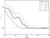Fig. B.1 Potential scale reduction factor R evaluated every ten samples for the parameters σint,0, σenv,0, χlum, and χred, as a function of the number of steps in the MCMC, for the scenario 2C1. The continuous and dashed lines represent a potential scale reduction factor equal to 1.0 and 1.1, respectively. It can be seen that the Gelman and Rubin test indicates convergence after a few thousand steps.

As an example, in Fig. B.1 we show the plot of the potential scale reduction factor R versus the number of steps for the Θ parameters in the scenario 2C1. The potential scale reduction factor has been evaluated every ten samples. After about 5000 steps we obtain R = 1 within a few percents. For each parameter of each test, we obtain R within a few percents¹⁰, which is sufficient to meet our convergence criteria. The aforementioned correlation coefficient ρ_j is calculated for each parameter j = σ_int,0, σ_env,0, χ_lum, and χ_red as follows,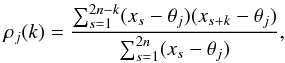${\mathit{\rho }}_{\mathit{j}}\mathrm{\left(}\mathit{k}\mathrm{\right)}\mathrm{=}\frac{{\sum }_{\mathit{s}\mathrm{=}\mathrm{1}}^{\mathrm{2}\mathit{n}\mathrm{-}\mathit{k}}\mathrm{(}{\mathit{x}}_{\mathit{s}}\mathrm{-}{\mathit{\theta }}_{\mathit{j}}\mathrm{)}\mathrm{(}{\mathit{x}}_{\mathit{s}\mathrm{+}\mathit{k}}\mathrm{-}{\mathit{\theta }}_{\mathit{j}}\mathrm{)}}{{\sum }_{\mathit{s}\mathrm{=}\mathrm{1}}^{\mathrm{2}\mathit{n}}\mathrm{(}{\mathit{x}}_{\mathit{s}}\mathrm{-}{\mathit{\theta }}_{\mathit{j}}\mathrm{)}}\mathit{,}$(B.4)where k is the number of steps and x_s is the value of one of these parameters for a given step. For all of the parameters in the scenario 2C1, l_c turns out to be ≈3000, while for the scenarios NPa and B2SP1a, the correlation length is about 500–1000. In these plots the steps in the burn-in phase have been discarded by visual inspection.

Appendix C: Alternative scenarios

In this Appendix, we present the application to scenarios including three components, representing:

• an intrinsic, an environmental, and aconstant contribution (scenario 3C),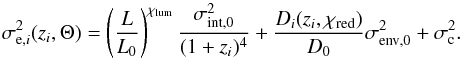${\mathit{\sigma }}_{\mathrm{e}\mathit{,i}}^{\mathrm{2}}\mathrm{\left(}{\mathit{z}}_{\mathit{i}}\mathit{,}\mathrm{\Theta }\mathrm{\right)}\mathrm{=}{\left(\frac{\mathit{L}}{{\mathit{L}}_{\mathrm{0}}}\right)}^{{\mathit{\chi }}_{\mathrm{lum}}}\frac{{\mathit{\sigma }}_{\mathrm{int}\mathit{,}\mathrm{0}}^{\mathrm{2}}}{\mathrm{(}\mathrm{1}\mathrm{+}{\mathit{z}}_{\mathit{i}}{\mathrm{)}}^{\mathrm{4}}}\mathrm{+}\frac{{\mathit{D}}_{\mathit{i}}\mathrm{\left(}{\mathit{z}}_{\mathit{i}}\mathit{,}{\mathit{\chi }}_{\mathrm{red}}\mathrm{\right)}}{{\mathit{D}}_{\mathrm{0}}}{\mathit{\sigma }}_{\mathrm{env}\mathit{,}\mathrm{0}}^{\mathrm{2}}\mathrm{+}{\mathit{\sigma }}_{\mathrm{c}}^{\mathrm{2}}\mathit{.}$(C.1)The constant contribution ${\mathit{\sigma }}_{\mathrm{c}}^{\mathrm{2}}$ takes into account terms that are not described by the parameterization of the other two but that could nevertheless be present in our data (e.g., the ionosphere, under the assumption that this does not show any direction dependence);

• an intrinsic, an environmental, and a latitude-dependent contribution (scenario LD), 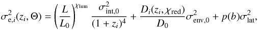${\mathit{\sigma }}_{\mathrm{e}\mathit{,i}}^{\mathrm{2}}\mathrm{\left(}{\mathit{z}}_{\mathit{i}}\mathit{,}\mathrm{\Theta }\mathrm{\right)}\mathrm{=}{\left(\frac{\mathit{L}}{{\mathit{L}}_{\mathrm{0}}}\right)}^{{\mathit{\chi }}_{\mathrm{lum}}}\frac{{\mathit{\sigma }}_{\mathrm{int}\mathit{,}\mathrm{0}}^{\mathrm{2}}}{\mathrm{(}\mathrm{1}\mathrm{+}{\mathit{z}}_{\mathit{i}}{\mathrm{)}}^{\mathrm{4}}}\mathrm{+}\frac{{\mathit{D}}_{\mathit{i}}\mathrm{\left(}{\mathit{z}}_{\mathit{i}}\mathit{,}{\mathit{\chi }}_{\mathrm{red}}\mathrm{\right)}}{{\mathit{D}}_{\mathrm{0}}}{\mathit{\sigma }}_{\mathrm{env}\mathit{,}\mathrm{0}}^{\mathrm{2}}\mathrm{+}\mathit{p}\mathrm{\left(}\mathit{b}\mathrm{\right)}{\mathit{\sigma }}_{\mathrm{lat}}^{\mathrm{2}}\mathit{,}$(C.2)where p(b) is the Galactic profile from Oppermann et al. (2015). The latitude-dependent contribution $\mathit{p}\mathrm{\left(}\mathit{b}\mathrm{\right)}{\mathit{\sigma }}_{\mathrm{lat}}^{\mathrm{2}}$ may explain a residual latitude dependence not taken into account in the modeling of Oppermann et al. (2015), e.g., an uncorrelated Galactic signal not captured by their analysis.

As for the simplest 2C-scenario, for each of these scenarios we run two tests corresponding to 41 632 and 4003 lines of sight. Figures C.1 and C.2 show the results when a third constant component (tests 3C1 and 3C2) and latitude-dependent component (tests LD1 and LD2) are included. In both figures, we show the plots for 41 632 lines of sight in panel a and for 4003 lines of sight in panel b.

These plots indicate that the algorithm also performs well when three components are considered. As expected, the values of the Θ parameters recovered are less accurate when a lower number of lines of sight is used. The additional parameters tend to lead to a slight increase in the posterior uncertainty for the other parameters when comparing with the results of 2C1 and 2C2.

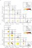Fig. C.1 As Fig. 2 but for results obtained with a three-component scenario, including a constant contribution, for 41 632 (3C1) lines of sight a) and 4003 (3C2) lines of sight b).

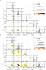Fig. C.2 As Fig. 2 but for results obtained with a three-component scenario, including a latitude-dependent contribution for 41 632 (LD1) lines of sight a) and 4003 (LD2) lines of sight b).

Appendix D: Priors

In order to get a data-driven solution and to keep our assumptions as general as possible, an uninformative prior should be adopted for the Θ parameters. Since we included all of the main redshift and luminosity dependencies in our model, the Gaussian prior in Eq. (21) is suitable for χ_lum and χ_red. Concerning σ_int,0 and σ_env,0, we may ask if different priors can have an impact on our results. In Sect. 3.1, we adopted a flat prior, 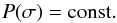$\mathit{P}\mathrm{\left(}\mathit{\sigma }\mathrm{\right)}\mathrm{=}\mathrm{const}\mathit{.}$(D.1)In this Appendix, we present two tests corresponding to extreme choices of these priors. Indeed, we considered a flat prior in σ² (scenario P1) 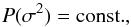$\mathit{P}\mathrm{\left(}{\mathit{\sigma }}^{\mathrm{2}}\mathrm{\right)}\mathrm{=}\mathrm{const}\mathit{.}\mathit{,}$(D.2)and a flat prior in ln(σ²) (scenario P0) 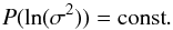$\mathit{P}\mathrm{\left(}\ln \mathrm{\right(}{\mathit{\sigma }}^{\mathrm{2}}\mathrm{\left)}\mathrm{\right)}\mathrm{=}\mathrm{const}\mathit{.}$(D.3)In Fig. D.1 we show the results for the two priors: flat in σ² in panel (a) and flat in ln(σ²) in panel b.

The first choice is an optimistic prior, since it implies a suppression of σ values ≪1, pushing for the recovery of larger, possibly ~1 values of σ. The second choice is a pessimistic prior since it would weight all small and large σ values in the same way, favoring negligible extragalactic contributions, easily compatible with the data because of the shape of the likelihood. We stress that the final results are not affected by the choice of the prior. However, this choice has an impact on the convergence time, since the starting point of each chain is randomly extracted from the prior. For example, for a flat prior in ln(σ²), the chances to extract a very small σ value (≪1) are larger than for the prior used in Sect. 3.1, possibly making the convergence time very long. For these tests, the number of lines of sight and the assumed noise properties are the same as in the 2C1 test.

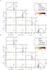Fig. D.1 As Fig. 2 but for results obtained with a two-component scenario and an overall extragalactic Faraday depth of ≈7.0 rad m-2 for a) a flat prior in σ2 (P1) and for b) a flat prior in ln(σ2) (P0) for 41 632 lines of sight.

All Tables

All Figures

	Fig. 1 Distribution of the real and mock samples of redshifts z (top) and flux densities FJy at 1.4 GHz (middle). In the bottom panel, flux density vs. redshift for sources with both measurements available (Taylor et al. 2009; Hammond et al. 2012).
In the text

Fig. 2 Results obtained with a two-component scenario for 41 632 (2C1) lines of sight in panel a) and for 4003 (2C2) in panel b). In each panel the top plots of each column show the one-dimensional projection of the posterior and the true value (dotted line), the outcome of the analysis (dashed and dash-dotted lines), and the prior (continuous line). The panels in color show the two-dimensional marginalized views of the posterior as sampled.

In the text

	Fig. 3 As Fig. 2 but for results obtained with a two-component scenario for LOFAR HBA observations for Nlos ≈ 2200 and an overall extragalactic standard deviation in Faraday depth of a) ≈7 rad m-2 (NPa) and b) ≈0.7 rad m-2 (NPb).
In the text

	Fig. 4 As Fig. 2 but for results obtained with a two-component scenario for SKA observations in the frequency range 650–1670 MHz for Nlos ≈ 3500 and an overall extragalactic Faraday rotation of a) ≈7.0 rad m-2 (B2SP1a) and b) ≈0.7 rad m-2 (B2SP1b).
In the text

	Fig. 5 As Fig. 2 but for results obtained with a two-component scenario for ASKAP observations in the frequency range 1130–1430 MHz for Nlos ≈ 3500 and an overall Faraday depth of ≈7.0 rad m-2 (POS).
In the text

Fig. 6 Uncertainty on σint,0, σenv,0, χlum, and χred (from the top to the bottom) as a function of the observational uncertainty σnoise and the number of lines of sight Nlos for an overall extragalactic Faraday depth variance of ≈7.0 rad m-2 (left panels) and ≈0.7 rad m-2 (right panels). The size of the points is proportional to the uncertainty on the parameter. A description of this uncertainty is given also by the grayscale. Circles refer to scenarios including two components, while triangles refer to three-component scenarios. Continuous lines correspond to ${\mathit{\sigma }}_{\mathrm{noise}}^{\mathrm{2}}\mathit{/}{\mathit{N}}_{\mathrm{los}}$ = const.

In the text

Fig. B.1 Potential scale reduction factor R evaluated every ten samples for the parameters σint,0, σenv,0, χlum, and χred, as a function of the number of steps in the MCMC, for the scenario 2C1. The continuous and dashed lines represent a potential scale reduction factor equal to 1.0 and 1.1, respectively. It can be seen that the Gelman and Rubin test indicates convergence after a few thousand steps.

In the text

	Fig. C.1 As Fig. 2 but for results obtained with a three-component scenario, including a constant contribution, for 41 632 (3C1) lines of sight a) and 4003 (3C2) lines of sight b).
In the text

	Fig. C.2 As Fig. 2 but for results obtained with a three-component scenario, including a latitude-dependent contribution for 41 632 (LD1) lines of sight a) and 4003 (LD2) lines of sight b).
In the text

	Fig. D.1 As Fig. 2 but for results obtained with a two-component scenario and an overall extragalactic Faraday depth of ≈7.0 rad m-2 for a) a flat prior in σ2 (P1) and for b) a flat prior in ln(σ2) (P0) for 41 632 lines of sight.
In the text

References

- Abazajian, K. N., Adelman-McCarthy, J. K., Agüeros, M. A., et al. 2009, ApJS, 182, 543 [NASA ADS] [CrossRef] [Google Scholar]
- Akahori, T., & Ryu, D. 2011, ApJ, 738, 134 [NASA ADS] [CrossRef] [Google Scholar]
- Akahori, T., Gaensler, B. M., & Ryu, D. 2014a, ApJ, 790, 123 [NASA ADS] [CrossRef] [Google Scholar]
- Akahori, T., Kumazaki, K., Takahashi, K., & Ryu, D. 2014b, PASJ, 66, 65 [NASA ADS] [Google Scholar]
- Bagchi, J., Enßlin, T. A., Miniati, F., et al. 2002, New Astron., 7, 249 [NASA ADS] [CrossRef] [Google Scholar]
- Bell, M. R., & Enßlin, T. A. 2012, A&A, 540, A80 [NASA ADS] [CrossRef] [EDP Sciences] [Google Scholar]
- Bernardi, G., de Bruyn, A. G., Brentjens, M. A., et al. 2009, A&A, 500, 965 [NASA ADS] [CrossRef] [EDP Sciences] [Google Scholar]
- Bernardi, G., Greenhill, L. J., Mitchell, D. A., et al. 2013, ApJ, 771, 105 [NASA ADS] [CrossRef] [Google Scholar]
- Bernet, M. L., Miniati, F., & Lilly, S. J. 2012, ApJ, 761, 144 [NASA ADS] [CrossRef] [Google Scholar]
- Bilicki, M., Peacock, J. A., Jarrett, T. H., Cluver, M. E., & Steward, L. 2014, Proc. IAU Symp., 308 [arXiv:1408.0799] [Google Scholar]
- Bonafede, A., Feretti, L., Murgia, M., et al. 2010, A&A, 513, A30 [NASA ADS] [CrossRef] [EDP Sciences] [Google Scholar]
- Braun, R., Oosterloo, T. A., Morganti, R., Klein, U., & Beck, R. 2007, A&A, 461, 455 [NASA ADS] [CrossRef] [EDP Sciences] [Google Scholar]
- Brentjens, M. A., & de Bruyn, A. G. 2005, A&A, 441, 1217 [NASA ADS] [CrossRef] [EDP Sciences] [Google Scholar]
- Broderick, A. E., Pfrommer, C., Puchwein, E., Chang, P., & Smith, K. M. 2014a, ApJ, 796, 12 [NASA ADS] [CrossRef] [Google Scholar]
- Broderick, A. E., Pfrommer, C., Puchwein, E., & Chang, P. 2014b, ApJ, 790, 137 [NASA ADS] [CrossRef] [Google Scholar]
- Brooks, S. P., & Gelman, A. 1997, J. Comput. Graph. Stat., 7, 434 [Google Scholar]
- Broten, N. W., MacLeod, J. M., & Vallee, J. P. 1988, Ap&SS, 141, 303 [NASA ADS] [CrossRef] [Google Scholar]
- Brown, J. C., Taylor, A. R., & Jackel, B. J. 2003, ApJS, 145, 213 [NASA ADS] [CrossRef] [Google Scholar]
- Brown, J. C., Haverkorn, M., Gaensler, B. M., et al. 2007, ApJ, 663, 258 [NASA ADS] [CrossRef] [Google Scholar]
- Burn, B. J. 1966, MNRAS, 133, 67 [NASA ADS] [CrossRef] [Google Scholar]
- Carilli, C. L., & Taylor, G. B. 2002, ARA&A, 40, 319 [NASA ADS] [CrossRef] [Google Scholar]
- Clarke, T. E. 2004, J. Korean Astron. Soc., 37, 337 [NASA ADS] [CrossRef] [Google Scholar]
- Clarke, T. E., Kronberg, P. P., Böhringer, H. 2001, ApJ, 547, L111 [NASA ADS] [CrossRef] [Google Scholar]
- Clegg, A. W., Cordes, J. M., Simonetti, J. M., & Kulkarni, S. R. 1992, ApJ, 386, 143 [NASA ADS] [CrossRef] [Google Scholar]
- Condon, J. J., Cotton, W. D., Greisen, E. W., et al. 1998, AJ, 115, 1693 [NASA ADS] [CrossRef] [Google Scholar]
- Condon, J. J., Cotton, W. D., & Broderick, J. J. 2002, AJ, 124, 675 [NASA ADS] [CrossRef] [Google Scholar]
- Dennison, B. 1979, AJ, 84, 725 [NASA ADS] [CrossRef] [Google Scholar]
- Donnert, J., Dolag, K., Lesch, H., Müller, E. 2009, MNRAS, 392, 1008 [NASA ADS] [CrossRef] [Google Scholar]
- Enßlin, T. A., Frommert, M., & Kitaura, F. S. 2009, Phys. Rev. D, 80, 105005 [NASA ADS] [CrossRef] [Google Scholar]
- Farnes, J. S., O’Sullivan, S. P., Corrigan, M. E., & Gaensler, B. M. 2014a, ApJ, 795, 63 [NASA ADS] [CrossRef] [Google Scholar]
- Farnes, J. S., Gaensler, B. M., & Carretti, E. 2014b, ApJS, 212, 15 [NASA ADS] [CrossRef] [Google Scholar]
- Farnsworth, D., Rudnick, L., & Brown, S. 2011, AJ, 141, 191 [NASA ADS] [CrossRef] [Google Scholar]
- Feain, I. J., Ekers, R. D., Murphy, T., et al. 2009, ApJ, 707, 114 [NASA ADS] [CrossRef] [Google Scholar]
- Feain, I. J., Cornwell, T. J., Ekers, R. D., et al. 2011, ApJ, 740, 17 [NASA ADS] [CrossRef] [Google Scholar]
- Feretti, L., Giovannini, G., Govoni, F., & Murgia, M. 2012, A&ARv, 20, 54 [Google Scholar]
- Gaensler, B. M., Dickey, J. M., McClure-Griffiths, N. M., et al. 2001, ApJ, 549, 959 [NASA ADS] [CrossRef] [Google Scholar]
- Gaensler, B. M., Haverkorn, M., Staveley-Smith, L., et al. 2005, Science, 307, 1610 [NASA ADS] [CrossRef] [PubMed] [Google Scholar]
- Gaensler, B. M., Landecker, T. L., Taylor, A. R., & POSSUM Collaboration 2010, BAAS, 42, 515 [NASA ADS] [Google Scholar]
- Gelman, A., & Rubin, D. B. 1992, Stat. Sci., 7, 457 [Google Scholar]
- Geman, S., & Geman, D. 1984, IEEE Trans. Pattern Analysis and Machine Intelligence, 6, 721 [CrossRef] [Google Scholar]
- Giovannini, G., Vacca, V., Girardi, M., et al. 2013, MNRAS, 435, 518 [NASA ADS] [CrossRef] [Google Scholar]
- Giovannini, G., Bonafede, A., Brown, S., et al. 2015, PoS(AASKA14) 104 [Google Scholar]
- Govoni, F., & Feretti, L. 2004, Int. J. Mod. Phys. D, 13, 1549 [NASA ADS] [CrossRef] [Google Scholar]
- Gregorini, L., Vigotti, M., Mack, K.-H., Zoennchen, J., & Klein, U. 1998, A&AS, 133, 129 [NASA ADS] [CrossRef] [EDP Sciences] [Google Scholar]
- Hahn, O., Porciani, C., Carollo, C. M., & Dekel, A. 2007, MNRAS, 375, 489 [NASA ADS] [CrossRef] [Google Scholar]
- Hales, C. A. 2013, ArXiv eprints [arXiv:1312.4602] [Google Scholar]
- Hales, C. A., Norris, R. P., Gaensler, B. M., & Middelberg, E. 2014, MNRAS, 440, 3113 [NASA ADS] [CrossRef] [Google Scholar]
- Hammond, A. M., Robishaw, T., & Gaensler, B. M. 2012, ArXiv eprints [arXiv:1209.1438] [Google Scholar]
- Hennessy, G. S., Owen, F. N., & Eilek, J. A. 1989, ApJ, 347, 144 [NASA ADS] [CrossRef] [Google Scholar]
- Harris, D. E., Stern, C. P., Willis, A. G., & Dewdney, P. E. 1993, AJ, 105, 769 [NASA ADS] [CrossRef] [Google Scholar]
- Hastings, W. K. 1970, Biometrika, 57, 1 [Google Scholar]
- Haverkorn, M., Gaensler, B. M., McClure-Griffiths, N. M., Dickey, J. M., & Green, A. J. 2006, ApJS, 167, 230 [CrossRef] [Google Scholar]
- Heald, G., Braun, R., & Edmonds, R. 2009, A&A, 503, 409 [NASA ADS] [CrossRef] [EDP Sciences] [Google Scholar]
- Ichiki, K., Takahashi, K., Ohno, H., Hanayama, H., & Sugiyama, N. 2006, Science, 311, 827 [NASA ADS] [CrossRef] [Google Scholar]
- Ideguchi, S., Takahashi, K., Akahori, T., Kumazaki, K., & Ryu, D. 2014, PASJ, 66, 5 [NASA ADS] [Google Scholar]
- Jasche, J., Kitaura, F. S., Li, C., & Enßlin, T. A. 2010, MNRAS, 409, 355 [NASA ADS] [CrossRef] [Google Scholar]
- Jelić, V., de Bruyn, A. G., Mevius, M., et al. 2014, A&A, 568, A101 [NASA ADS] [CrossRef] [EDP Sciences] [Google Scholar]
- Johnston-Hollitt, M. 2003, Ph.D. Thesis [Google Scholar]
- Johnston-Hollitt, M., & Ekers, R. D. 2004, ArXiv eprints [arXiv:astro-ph/0411045] [Google Scholar]
- Johnston-Hollitt, M., Govoni, F., Beck, R., et al. 2015, PoS(AASKA14)092 [Google Scholar]
- Kato, T., Tabara, H., Inoue, M., & Aizu, K. 1987, Nature, 329, 223 [NASA ADS] [CrossRef] [Google Scholar]
- Kim, K.-T., Tribble, P. C., & Kronberg, P. P. 1991, ApJ, 379, 80 [NASA ADS] [CrossRef] [Google Scholar]
- Klein, U., Mack, K.-H., Gregorini, L., & Vigotti, M. 2003, A&A, 406, 579 [NASA ADS] [CrossRef] [EDP Sciences] [Google Scholar]
- Kronberg, P. P., & Perry, J. J. 1982, ApJ, 263, 518 [NASA ADS] [CrossRef] [Google Scholar]
- Kronberg, P. P., Kothes, R., Salter, C. J., & Perillat, P. 2007, ApJ, 659, 267 [NASA ADS] [CrossRef] [Google Scholar]
- Kronberg, P. P., Bernet, M. L., Miniati, F., et al. 2008, ApJ, 676, 70 [NASA ADS] [CrossRef] [Google Scholar]
- Kumazaki, K., Akahori, T., Ideguchi, S., Kurayama, T., & Takahashi, K. 2014, PASJ, 66, 61 [NASA ADS] [Google Scholar]
- Lawler, J. M., & Dennison, B. 1982, ApJ, 252, 81 [NASA ADS] [CrossRef] [Google Scholar]
- Leclercq, F., Jasche, J., & Wandelt, B. 2015, A&A, 576, L17 [NASA ADS] [CrossRef] [EDP Sciences] [Google Scholar]
- Mauch, T., & Sadler, E. M. 2007, MNRAS, 375, 931 [NASA ADS] [CrossRef] [Google Scholar]
- Mao, S. A., Gaensler, B. M., Stanimirović, S., et al. 2008, ApJ, 688, 1029 [NASA ADS] [CrossRef] [Google Scholar]
- Mao, S. A., Gaensler, B. M., Haverkorn, M., et al. 2010, ApJ, 714, 1170 [NASA ADS] [CrossRef] [Google Scholar]
- McClure-Griffiths, N. M., Dickey, J. M., Gaensler, B. M., et al. 2005, ApJS, 158, 178 [NASA ADS] [CrossRef] [Google Scholar]
- Metropolis, N., Rosenbluth, A. W., Rosenbluth, M. N., Teller, A. H., & Teller, E. 1953, J. Chem. Phys., 21, 6 [Google Scholar]
- Minter, A. H., & Spangler, S. R. 1996, ApJ, 458, 194 [NASA ADS] [CrossRef] [Google Scholar]
- Mulcahy, D. D., Horneffer, A., Beck, R., et al. 2014, A&A, 568, AA74 [NASA ADS] [CrossRef] [EDP Sciences] [Google Scholar]
- Neronov, A., & Vovk, I. 2010, Science, 328, 73 [NASA ADS] [CrossRef] [PubMed] [Google Scholar]
- Offringa, A. R., de Bruyn, A. G., Zaroubi, S., et al. 2013, A&A, 549, AA11 [Google Scholar]
- Oppermann, N., Junklewitz, H., Robbers, G., et al. 2012, A&A, 542, A93 [NASA ADS] [CrossRef] [EDP Sciences] [Google Scholar]
- Oppermann, N., Junklewitz, H., Greiner, M., et al. 2015, A&A, 575, A118 [NASA ADS] [CrossRef] [EDP Sciences] [Google Scholar]
- Oren, A. L., & Wolfe, A. M. 1995, ApJ, 445, 624 [NASA ADS] [CrossRef] [Google Scholar]
- Planck Collaboration XVI. 2014, A&A, 571, A16 [NASA ADS] [CrossRef] [EDP Sciences] [Google Scholar]
- Planck Collaboration XIX. 2016, A&A, in press DOI: 10.1051/0004-6361/201525821 [Google Scholar]
- Pshirkov, M. S., Tinyakov, P. G., & Urban, F. R. 2015, Phys. Rev. Lett., 116, 191302 [Google Scholar]
- Roy, S., Rao, A. P., & Subrahmanyan, R. 2005, MNRAS, 360, 1305 [NASA ADS] [CrossRef] [Google Scholar]
- Rudnick, L., & Jones, T. W. 1983, AJ, 88, 518 [NASA ADS] [CrossRef] [Google Scholar]
- Schnitzeler, D. H. F. M. 2010, MNRAS, 409, L99 [NASA ADS] [Google Scholar]
- Selig, M., Bell, M. R., Junklewitz, H., et al. 2013, A&A, 554, A26 [NASA ADS] [CrossRef] [EDP Sciences] [Google Scholar]
- Simard-Normandin, M., Kronberg, P. P., & Button, S. 1981, ApJS, 45, 97 [NASA ADS] [CrossRef] [Google Scholar]
- Sotomayor-Beltran, C., Sobey, C., Hessels, J. W. T., et al. 2013, A&A, 552, A58 [NASA ADS] [CrossRef] [EDP Sciences] [Google Scholar]
- Stasyszyn, F., Nuza, S. E., Dolag, K., Beck, R., & Donnert, J. 2010, MNRAS, 408, 684 [NASA ADS] [CrossRef] [Google Scholar]
- Stepanov, R., Arshakian, T. G., Beck, R., Frick, P., & Krause, M. 2008, A&A, 480, 45 [NASA ADS] [CrossRef] [EDP Sciences] [Google Scholar]
- Tabara, H., & Inoue, M. 1980, A&AS, 39, 379 [Google Scholar]
- Takahashi, K., Ichiki, K., Ohno, H., & Hanayama, H. 2005, Phys. Rev. Lett., 95, 121301 [NASA ADS] [CrossRef] [PubMed] [Google Scholar]
- Takahashi, K., Mori, M., Ichiki, K., & Inoue, S. 2012, ApJ, 744, L7 [Google Scholar]
- Takahashi, K., Mori, M., Ichiki, K., Inoue, S., & Takami, H. 2013, ApJ, 771, L42 [NASA ADS] [CrossRef] [Google Scholar]
- Tavecchio, F., Ghisellini, G., Foschini, L., et al. 2010, MNRAS, 406, L70 [NASA ADS] [Google Scholar]
- Taylor, A. R., Gibson, S. J., Peracaula, M., et al. 2003, AJ, 125, 3145 [NASA ADS] [CrossRef] [Google Scholar]
- Taylor, A. R., Stil, J. M., & Sunstrum, C. 2009, ApJ, 702, 1230 [NASA ADS] [CrossRef] [Google Scholar]
- Uyaniker, B., & Landecker, T. L. 2002, ApJ, 575, 225 [NASA ADS] [CrossRef] [Google Scholar]
- Vacca, V., Oppermann, N., Ensslin, T., et al. 2015, PoS(AASKA14) 114 [Google Scholar]
- Vallée, J. P., MacLeod, M. J., & Broten, N. W. 1986, A&A, 156, 386 [NASA ADS] [Google Scholar]
- Van Eck, C. L., Brown, J. C., Stil, J. M., et al. 2011, ApJ, 728, 97 [NASA ADS] [CrossRef] [Google Scholar]
- Vigotti, M., Gregorini, L., Klein, U., & Mack, K.-H. 1999, A&AS, 139, 359 [NASA ADS] [CrossRef] [EDP Sciences] [Google Scholar]
- Wandelt, B. D., Larson, D. L., & Lakshminarayanan, A. 2004, Phys. Rev. D, 70, 083511 [NASA ADS] [CrossRef] [Google Scholar]
- Welter, G. L., Perry, J. J., & Kronberg, P. P. 1984, ApJ, 279, 19 [NASA ADS] [CrossRef] [Google Scholar]
- Wolleben, M., & Reich, W. 2004, A&A, 427, 537 [NASA ADS] [CrossRef] [EDP Sciences] [Google Scholar]
- Wrobel, J. M. 1993, AJ, 106, 444 [NASA ADS] [CrossRef] [Google Scholar]
- Xu, H., Li, H., Collins, D. C., Li, S., & Norman, M. L. 2010, ApJ, 725, 2152 [NASA ADS] [CrossRef] [Google Scholar]
- Xu, H., Li, H., Collins, D. C., Li, S., & Norman, M. L. 2011, ApJ, 739, 77 [NASA ADS] [CrossRef] [Google Scholar]
- Zaroubi, S., Jelić, V., de Bruyn, A. G., et al. 2015, MNRAS, 454, L46 [NASA ADS] [Google Scholar]