| Issue |
A&A
Volume 590, June 2016
|
|
|---|---|---|
| Article Number | A61 | |
| Number of page(s) | 16 | |
| Section | Extragalactic astronomy | |
| DOI | https://doi.org/10.1051/0004-6361/201628347 | |
| Published online | 11 May 2016 | |
Exploring the nature of the broadband variability in the flat spectrum radio quasar 3C 273
1
Max-Planck-Institut für Radioastronomie (MPIfR),
Auf dem Hügel 69, 53121
Bonn,
Germany
e-mail:
This email address is being protected from spambots. You need JavaScript enabled to view it.
2
Instituto de Radioastronomía Milimétrica (IRAM),
Avenida Divina Pastora 7, Local
20, 18012
Granada,
Spain
3
Department of Physical Science, Hiroshima
University, Higashi-Hiroshima,
739-8526
Hiroshima,
Japan
4
Hiroshima Astrophysical Science Center, Hiroshima
University, Higashi-Hiroshima,
739-8526
Hiroshima,
Japan
5
Institute for Astrophysical Research, Boston
University, 725 Commonwealth
Avenue, Boston,
MA
02215,
USA
6
Harvard-Smithsonian Center for Astrophysics,
Cambridge, MA
02138,
USA
7
Astronomical Observatory of National Taras Shevchenko University
of Kiev, 01601
Kiev,
Ukraine
Received: 19 February 2016
Accepted: 24 March 2016
Abstract
The detailed investigation of the broadband flux variability in the blazar 3C 273 allowed us to probe the location and size of emission regions and their physical conditions. We conducted correlation studies of the flaring activity in 3C 273, which was observed for the period between 2008 and 2012. The observed broadband variations were investigated using the structure function and the discrete correlation function methods. Starting from the commonly used power spectral density (PSD) analysis at X-ray frequencies, we extended our investigation to characterise the nature of variability at radio, optical, and γ-ray frequencies. The PSD analysis showed that the optical and infrared light-curve slopes are consistent with the slope of white-noise processes, while the PSD slopes at radio, X-ray, and γ-ray energies are consistent with red-noise processes. We found that the estimated fractional variability amplitudes strongly depend on the observed frequency. The flux variations at γ-ray and mm-radio bands are found to be significantly correlated. Using the estimated time lag of (110 ± 27) days between γ-ray and radio light-curves, where γ-ray variations lead the radio bands, we constrained the location of the γ-ray emission region at a de-projected distance of 1.2 ± 0.9 pc from the jet apex. Flux variations at X-ray bands were found to have a significant correlation with variations at both radio and γ-ray energies. The correlation between X-ray and γ-ray light curves indicates two possible time lags, which suggests that two components are responsible for the X-ray emission. A negative time lag of −(50 ± 20) days, where the X-rays are leading the emission, suggests that X-rays are emitted closer to the jet apex from a compact region (0.02–0.05 pc in size), most likely from the corona at a distance of (0.5 ± 0.4) pc from the jet apex. A positive time lag of (110 ± 20) days (γ-rays are leading the emission) suggests a jet-base origin of the other X-ray component at ~4 to 5 pc from the jet apex. The flux variations at radio frequencies were found to be well correlated with each other such that the variations at higher frequencies are leading the lower frequencies, which is expected from the standard shock-in-jet model.
Key words: galaxies: active / quasars: individual: 3C 273 / galaxies: jets / gamma rays: galaxies / radio continuum: galaxies
Master student at the Argelander Institut für Astronomie (AIfA) – University of Bonn.
© ESO, 2016
1. Introduction
The flat spectrum radio quasar (FSRQ) 3C 273 has been one of the most frequently studied quasars since its discovery in 1963. It is a nearby source with a redshift of 0.158 (Schmidt 1963). It is characterised by a jet close to the line of sight at a viewing angle of 5°−11° (Liu & Shen 2009) and a highest superluminal apparent velocity of vapp = 15c (Lister et al. 2013). The jet remains collimated in all wavebands from radio to X-rays, although it extends to kpc scales. This allows a detailed study of the physical properties of the AGN starting from regions close to the supermassive black hole (SMBH) to the outer jet regions (Uchiyama et al. 2006).
The blazar 3C 273 is characterised by a strong radio emission from mm- to cm-wavelengths (Soldi et al. 2008). It has been suggested that this radio emission is caused by synchrotron emission of relativistic electrons in the jet, which could emit up to infrared (IR) frequencies (McHardy et al. 1999; Soldi et al. 2008). Türler et al. (1999) found that the sub-mm to radio flaring activity of the source agrees with the shock-in-jet model suggested by Marscher & Gear (1985). They also found that the high-frequency radio outbursts are short-lived and come from a region closer to the jet apex than the long-lived low-frequency radio outbursts.
Unlike other blazars that are highly polarised, 3C 273 has an average polarisation degree below 1% at optical frequencies (Valtaoja et al. 1991). The source is characterised by a blue bump that is due to the excess in the optical/UV emission. Two possible components have been suggested to explain the complex optical/UV spectrum. One rapidly variable component might stem from the accretion disk (Shields 1978; Soldi et al. 2008) or illumination by an X-ray source (Ross & Fabian 1993) or a hot corona (Haardt et al. 1994). The second component seems to be related to synchrotron emission from the jet (Paltani et al. 1998). The IR emission in 3C 273 seems to be due to two variable components (Paltani et al. 1998), where one component is due to thermal emission from the dusty torus and the other component to synchrotron emission from the jet (Robson et al. 1993; McHardy et al. 1999; Sokolov & Marscher 2005).
The source exhibits significant variations in the X-ray regime. Several studies have been carried out to understand the emission mechanisms and locate the radiation regions. Studies by McHardy et al. (1999), Grandi & Palumbo (2004), McHardy et al. (2007) suggested that a Seyfert-like component from the accretion disk is responsible for about 20% of the X-ray emission, while the rest might be due to synchrotron self-Compton processes, most likely the up-scattering of the IR photons that had been produced by the synchrotron emission of the jet. Alternatively, the X-ray emission might be due to the Comptonisation of the UV photons (Madsen et al. 2015). The weak and neutral iron line in the X-ray spectrum suggests that the X-ray emission arises from the corona and is reflected off the accretion disk (Madsen et al. 2015). The source therefore exhibits Seyfert-like properties in the X-ray regime (McHardy et al. 1999; Grandi & Palumbo 2004).
A previous study carried out on the multi-wavelength variability of 3C 273 found a correlation between the X-ray and the IR flares, with the latter leading the former by a time lag of (0.75 ± 0.25) days (McHardy et al. 1999). This rules out the external Compton (EC) emission process as possible producer of X-ray emission. This correlation was later confirmed by McHardy et al. (2007). Chernyakova et al. (2007) found a correlation between UV and X-rays, but this correlation is still debated because some studies that failed to confirm this correlation (Walter & Courvoisier 1992; Soldi et al. 2008). Many studies found a strong correlation between radio and γ-rays for some sources (Beaklini & Abraham 2014; Max-Moerbeck et al. 2014; Ramakrishnan et al. 2015). Moreover, the gamma-ray flares were accompanied by the ejection of new components from the base of the jet (Jorstad et al. 2012).
The source was first detected in γ-ray frequencies by COS-B in 1970. The Energetic Gamma-ray Experiment Telescope (EGRET) onboard the Compton Gamma-Ray Observatory (CGRO) detected the source in 1991 at energies higher than 100 MeV (Hartman et al. 1992). The Fermi-LAT (Large Area Telescope) detected 3C 273 from the beginning of its operation in 2008 (Abdo et al. 2010). Between July 2009 and April 2010, a strong flaring activity on GeV scales was reported. A ten-day flare was observed in August 2009, which was followed by two bright flares on 15–19 and 20–23 September 2009. A sequence of rapid flares followed these two initial flares. The last flare was observed in April 2010, and since then, the source went into a quiescent state that is lasting until the present day (Rani et al. 2013b). The fastest γ-ray flare had a doubling timescale of 1.1 h (Rani et al. 2013b). Following the episodes of extreme flaring activity in the source since 2008 (Rani et al. 2013b), we investigate the nature of the observed broadband flaring activity. We carried out a detailed cross-correlation investigation across the electromagnetic spectrum to provide better constraints on the emission mechanisms. The key objective is to provide a better constraint on the location and size of the emission region.
This paper is structured as follows. In Sect. 2 we explain the data we used. Section 3 presents the light curves, and we explain the methods we applied, followed by the results of each method. We discuss the results in Sect. 4 and conclude in Sect. 5.
2. Observations and data reduction
To explore the broadband flaring activity, we monitored the source with both space- and ground-based observing facilities between May 2008 and March 2012 (MJD = 54 600 to 56 000). In the following subsections, we summarise the observations and data reduction.
2.1. Gamma-ray data
The high-energy GeV observations were obtained in survey mode by Fermi-LAT. The data cover an energy range from 100 MeV to 300 GeV. Here we used the weekly and monthly averaged data of 3C 273 that have been presented in Rani et al. (2013b), where the details of the observations and data reduction are discussed.
2.2. X-ray data
X-ray observations of the source were obtained by two space-based instruments: Swift and the Rossi X-ray Timing Explorer (RXTE). The X-ray light curves cover three energy bands. The monthly averaged hard X-ray light curve, covering an energy range between 14−192 keV, was observed by the Swift-Burst Alert Telescope (BAT)1 in both photon-counting (PC) and windowed-timing (WT) modes. Details of the observations and data reduction2 are given in Stroh & Falcone (2013). Observations at 2−10 keV and 10−50 keV X-ray bands are provided by the Rossi X-ray Timing Explorer – Proportional Counter Array (RXTE-PCA)3. The data are available for public use4. Details about the instrument and data reduction5 are presented in Jahoda (1994).
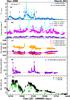 |
Fig. 1 Broadband light curves of 3C 273: a) weekly (turquoise circles) and monthly (blue circles) averaged γ-ray light curves; b) 14–192 keV band (cyan), the 10–50 keV band (indigo) and the 2–10 keV band (magenta) X-ray light curves; c) optical (V and R passbands) and IR (J passband) light curves; d) optical percentage polarisation curve; and e) radio flux density curves at 230 GHz (in black) and 350 GHz (in green) bands. |
2.3. Optical and IR data
Optical and IR light curves were provided by the Small and Moderate Aperture Research Telescope System (SMARTS) monitoring programme6. SMARTS observes with telescopes located at the Cerro Tololo Inter-American Observatory (CTIO). The monitoring programme aims to understand the high-energy emission of blazars by searching for a temporal correlation between flux and spectra of the main emission components. The observation and data reduction of the light curves is reported in Bonning et al. (2012). Observations made with the 2.3 m Bok Telescope of the Steward Observatory7 complemented the optical data. The Steward Observatory provides optical data in R and V-bands for the Fermi blazars. Details about the light curves produced in the Steward Observatory are presented in Smith et al. (2009). The polarisation measurements are derived from the median Stokes Q and U values found from spectropolarimetry in a 5000–7000 Å bin. We also used optical photometric data from the Kanata Telescope at the Hiroshima Observatory8. Details about the telescope and its instruments are given in Uemura & Kanata Team (2009). Details of the observation and data reduction of the light curves are reported in Ikejiri et al. (2011).
2.4. Radio data
Radio band observations at 2.6, 5, 8, 10, 15, 23, 32, 43, 86, and 142 GHz were provided by the Fermi/GST AGN Multi-frequency Monitoring Alliance (F-GAMMA) programme 9 (Fuhrmann et al. 2007; Angelakis et al. 2008). The F-GAMMA programme uses the Effelsberg 100 m telescope, which covers a range from 2.6 to 43 GHz, and the IRAM 30 m telescope at 86 and 142 GHz at the Pico Veleta Observatory. The millimetre observations are closely coordinated with the more general flux density monitoring conducted by IRAM, and data from both programmes are included in this paper. The 230 and 350 GHz light curves are provided by the SMA Observer Centre data base10 (Gurwell et al. 2007).
3. Analysis and results
In this section, we present the statistical analysis of the observed broadband variations in 3C 273. We compare the fractional variability in each band as well as the variability timescale. To quantify the correlation between different frequencies, we employed the cross-correlation function method. Finally, we used the power spectral density (PSD) method to gain a better insight into the nature of the variability by describing the amount of variability as a function of temporal frequency. The significance of the obtained results was tested through simulations. In the following sub-sections, we discuss the analysis and results in detail.
3.1. Light-curve analysis
Figures 1–3 show the broadband light curves of 3C 273. Panel (a) of Fig. 1 shows the monthly averaged γ-ray light curve superimposed on top of the weekly averaged curve. The monthly sampled light curve shows fewer flares (labelled 1 to 4) than the weekly sampled light curve. Apparently, the source exhibits two different modes of flaring activity. A mode of slow activity (between MJD = 54 600 to 55 000) is followed by a second phase that is characterised by rapid and strong flaring activity (flares A to E) between 55 050 and 55 300 MJD. The source went to a quiescent state after flare E observed in April 2010, which still persists. The source also exhibited significant spectral variations during the flaring activity. At the beginning of each flare, the spectrum becomes harder and then softens again at the end of the flare (Rani et al. 2013b).
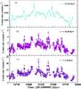 |
Fig. 2 X-ray light curves of 3C 273 at 14−192 keVa), 10−50 keVb), and 2−10 keVc). |
Similarly to the γ-ray regime, the source was active in X-ray bands (see Fig. 1b). Apparently, the flaring activity is very similar in the three observed X-ray bands (Fig. 2). As seen for the Swift-BAT light curve, there is a major flare that was observed almost simultaneously with flare (C) in the γ-ray flares. However, when the source went to a quiet state in the γ-ray regime, it continued to flare at X-ray frequencies.
Figure 1c shows the optical (R and V passbands) and IR (J passband) light curves. Unlike at γ-ray and X-ray energies, the optical/IR light curves of the source show fluctuations with a lower amplitude and without pronounced peaks. The light curves have an almost constant flux during the entire period of observation. In addition, the observed optical fractional polarisation is quite low (<2%). We noted significant variations in the polarisation curve (Fig. 1d), which are indicative of an underlying non-thermal variable emission component. Apparently, the variations in optical polarisation became more pronounced during the γ-ray flaring activity. When the source went into a quiescent state in the GeV regime, no pronounced activity was noted in the percentage polarisation curve.
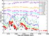 |
Fig. 3 Radio (cm to mm) band light curves of 3C 273. Different colours represent different frequencies, from 2.6 GHz to 350 GHz (from top to bottom). |
Figure 1e shows the light curves at 230 and 350 GHz to compare the variability of the mm-band with the variability in other energy bands. Figure 3 shows all radio band light-curves of the source. Higher radio frequencies from 23 GHz to 350 GHz show two flares: flare ℛ1 between 54 600 and 55 050 MJD, and flare ℛ2 between 55 050 and 55 600 MJD. At 230 and 350 GHz radio bands, we also note sub-flaring activity on short timescales that is superimposed on the main flare ℛ1. This flare is observed simultaneously with flares 1 and 2 in the GeV regime, while flare ℛ2 is observed during the strong flaring period between 55 000 and 55 300 MJD at γ-ray frequencies. The flaring activity is less pronounced at frequencies below 23 GHz, which might be due to opacity. It is important to note that when the source was quiet in the GeV regime, the radio light-curves did not show any prominent variations.
3.2. Fractional variability
We computed the fractional variability amplitude to compare the variations at different energy bands. Following Vaughan et al. (2003), we define the fractional variability as follows: 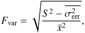 (1)where S2 is the variance of the light curve,
  is the mean value of the flux in the light curve, and
  its mean square error. The formal error of the fractional variability is estimated by (Vaughan et al. 2003, Appendix B)
  (2)where err is the error on the flux. We adopted this method because it takes the uncertainty on the flux in account to calculate the variability amplitude and the error on it. By applying Eq. (1), we obtained an estimate of the fractional variability of all the light curves available for 3C 273. The estimated Fvar amplitudes for the broadband light curves are plotted in Fig. 4.
 |
Fig. 4 Fractional variability amplitude plotted as a function of frequency. The red (black) point shows the fractional variability amplitude of the monthly (weekly) averaged γ-ray light curve. |
Figure 4 shows that the variability amplitude for the radio light-curves tends to increase with increasing frequency. This might be explained in terms of opacity effects: at higher frequencies, we probe the optically thin regions in the jet. There is less significant variability in the optical and IR light curves; as a consequence, the estimated fractional variability amplitudes at these bands are comparatively low. This might also be caused by the lack of data around the GeV flaring times. The fractional variability amplitude increases again in the X-ray regime and is similar to the fractional variability amplitude at mm-radio bands. The estimated Fvar amplitudes are significantly higher (≥100%) for the γ-ray light curves.
3.3. Structure function
We used the structure function (SF) method (Simonetti et al. 1985) to calculate the characteristic variability timescales in the light curves. For a given time series, the structure function (Simonetti et al. 1985) is defined as ![Mathematical equation: \begin{equation} SF(\Delta t)=\frac{1}{N}\sum_{i=1}^{N}\left[x_{i}-x_{i+\Delta t}\right]^{2} , \end{equation}](/articles/aa/full_html/2016/06/aa28347-16/aa28347-16-eq36.png) (3)where xi is the flux at a given time, xi + Δt is the flux at a time separation of Δt, and N is the number of data points that share the same Δt separation within a binning time interval. It is important to note that the SF breaks are not always reliable indicators of variability timescales (Emmanoulopoulos et al. 2010). We therefore used the SF method only for comparison purposes; the estimated timescales were not used for any further calculations. Using Eq. (3), we extracted the variability for all the light curves. The SF curves at 230 GHz and 2–10 keV bands are shown in Fig. 5; the SF curves for the remainder are shown in Fig. A.3.
(3)where xi is the flux at a given time, xi + Δt is the flux at a time separation of Δt, and N is the number of data points that share the same Δt separation within a binning time interval. It is important to note that the SF breaks are not always reliable indicators of variability timescales (Emmanoulopoulos et al. 2010). We therefore used the SF method only for comparison purposes; the estimated timescales were not used for any further calculations. Using Eq. (3), we extracted the variability for all the light curves. The SF curves at 230 GHz and 2–10 keV bands are shown in Fig. 5; the SF curves for the remainder are shown in Fig. A.3.
The 230 GHz SF curve (Fig. 5) shows that the SF values increase as a function of time lag and reach a peak that is followed by a dip. The first SF peak corresponds to the shortest variability timescale, and the dip indicates a possible periodic variation timescale, if it is repeated (see Rani et al. 2009, for details). The estimated variability timescales at different energy bands are listed in Table 1. For the error on the time lag, we adopted half of the time binning as a conservative estimate.
Figure 6 shows that the variability timescales at radio bands decrease at higher frequencies. This implies that we probe compact emission regions at short-mm bands, which are opaque to cm radio bands. The fractional variability is very low in the optical bands. The variability timescales therefore cannot be determined with accuracy.
 |
Fig. 5 Structure function at the 230 GHz radio band (top) and 2–10 keV X-ray band (bottom). |
The variability timescales for the three X-ray light curves are very similar. We found a timescale of (226 ± 15) days for the light curves at 2–10 keV and 10–50 keV bands and a timescale of (228 ± 15) days for the X-ray bands at 14–192 keV. These X-ray variability timescales are similar to the variability timescales at mm-radio bands. In addition, we noted multiple cycles in the SF curves at both mm-radio and X-ray bands (see Fig. 5), which suggests nearly periodic variations at timescales of 350–400 days. Similar timescales for variability and quasi-periodic oscillations at short-mm radio and X-ray regimes suggest that they might be correlated.
Using the SF analysis of the weekly averaged γ-ray light curve, we found a variability timescale of (91 ± 10) days. However, it is important to note that the SF gives the timescale of the long-term behaviour of the light curve. Interestingly, the estimated γ-ray variability timescale is similar to that at 86 and 142 GHz radio bands (see Table 1), which might be an indication of a possible correlation between the radio and γ-ray bands. We investigate this in detail in Sect. 3.5.
Variability timescales as derived from the structure function analysis.
 |
Fig. 6 Variability timescales plotted as a function of frequency (Hz). |
3.4. Power spectral density (PSD)
To explore the nature of the variability, we used the PSD analysis method (Vaughan et al. 2003; Vaughan 2005). For an evenly sampled data set, the periodogram is the modulus-squared of the discrete Fourier transform (DFT) of the data. In a light curve with flux series xi measured at discrete times ti (i = 1,2,...,N), the modulus-square of the DFT is given as  (4)at
(4)at  evenly spaced temporal frequencies
  , where
  . The Nyquist frequency is
  . The periodogram I(fj) is given by
 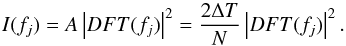 (5)The periodogram will be scattered around the true underlying power spectrum if we are observing a noise process, following a χ2 distribution with two degrees of freedom. The true power spectrum P(fj) is calculated as
 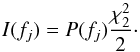 (6)
(6)
3.4.1. Fitting the periodogram
The underlying power density spectrum can be described by a power law P(f) = Nf−a, where a is the slope and N is the normalisation constant. We fitted the power law to the PSD using a least-squares fit method (LS) in log-scale. The scatter is multiplicative in linear-space, therefore it is additive in log-space and identical at each frequency (Geweke & Porter-Hudak 1989; Papadakis & Lawrence 1993): ![Mathematical equation: \begin{equation} \log\left[I(f_{j})\right]=\log\left[{P}(f_{j})\right]+\log\left[\frac{\chi_{2}^{2}}{2}\right] \cdot \end{equation}](/articles/aa/full_html/2016/06/aa28347-16/aa28347-16-eq73.png) (7)Nonetheless, the expectation value of the periodogram in log-space is not the same as the expectation value of the spectrum. There is a bias between the two values. This bias is a constant because of the shape of the
(7)Nonetheless, the expectation value of the periodogram in log-space is not the same as the expectation value of the spectrum. There is a bias between the two values. This bias is a constant because of the shape of the  -distribution in log-space, and it can be trivially removed,
 ![Mathematical equation: \begin{equation} \left\langle \log\left[I(f_{j})\right]\right\rangle =\left\langle \log\left[\ensuremath{{P}(f_{j})}\right]\right\rangle +\left\langle \log\left[\ensuremath{\frac{\ensuremath{\chi_{2}^{2}}}{2}}\right]\right\rangle \cdot \end{equation}](/articles/aa/full_html/2016/06/aa28347-16/aa28347-16-eq75.png) (8)Based on Abramowitz & Stegun (1964), the estimate of this bias constant is then
(8)Based on Abramowitz & Stegun (1964), the estimate of this bias constant is then ![Mathematical equation: \hbox{$\left\langle \log\left[\ensuremath{\frac{\ensuremath{\chi_{2}^{2}}}{2}}\right]\right\rangle = -0.25068...$}](/articles/aa/full_html/2016/06/aa28347-16/aa28347-16-eq76.png) , which gives
, which gives ![Mathematical equation: \begin{equation} \left\langle \log\left[\ensuremath{{P}(f_{j})}\right]\right\rangle =\left\langle \log\left[I(f_{j})\right]\right\rangle +0.25068 . \end{equation}](/articles/aa/full_html/2016/06/aa28347-16/aa28347-16-eq77.png) (9)This method is suitable for evenly sampled data, which is not the case of our data. Therefore, we first interpolated the data using a cubic spline interpolation method, and then applied the PSD method on the interpolated light curves. Since the data were manipulated, we tested our results through simulations.
(9)This method is suitable for evenly sampled data, which is not the case of our data. Therefore, we first interpolated the data using a cubic spline interpolation method, and then applied the PSD method on the interpolated light curves. Since the data were manipulated, we tested our results through simulations.
3.4.2. Simulations
We tested the significance level of the obtained results through a simulation. The most frequently used method is the Timmer & König method for light-curve simulations (Timmer & Koenig 1995). This method uses a Gaussian distribution to simulate the light curves, which is not the case of the blazar light curves. The burst-like events in blazars deviate considerably from such a distribution and are better described with a gamma- or log-normal distribution. This has been taken into account by Emmanoulopoulos et al. (2013). We here simulated the light curves using the Emmanoulopoulos method with the implementation11 of Connolly (2015).
The code calculates the probability density function (PDF) of a given light curve. The estimated PDF is then fitted using a combination of a gamma- and a log-normal distribution. The code also estimates the slope and the normalisation of the PSD through a broken power-law model. However, these estimates are not reported here because we used a simple power-law fit for our PSD fits. Using the best-fit parameters and the slope and normalisation of the PSD, the code simulates a number of light curves that have a PDF similar to the PDF of the original light curve.
3.4.3. PSD parameter test
To test our results, a raw fitting of the original PSD was made using the function P(f) = Nf−a, (where a is the slope and N the normalisation). After setting the slope and the normalisation as variable in the simulation algorithm (see Sect. 3.4.2), an interval for each was defined with an appropriate increment. The next step sampled the simulated light curves at the same bin width as the observed ones. For each combination of slope and normalisation, we simulated two hundred light curves. We calculated the PSD of each of these light curves and calculated the mean and standard deviation of the two hundred PSDs as well.
The final step was then to find the combination whose mean best fits the original PSD and minimises the value of the chi-square (Uttley et al. 2002), ![Mathematical equation: \begin{equation} \chi_{\rm dist}^{2}=\sum_{\nu=\nu_{\rm min}}^{\nu_{\rm max}}\frac{\left[\overline{P_{\rm sim}(\nu)}-P_{\rm obs}(\nu)\right]^{2}}{\Delta\overline{P_{\rm sim}(\nu)^{2}}} \cdot \end{equation}](/articles/aa/full_html/2016/06/aa28347-16/aa28347-16-eq79.png) (10)By finding the combination that has a minimum chi-square value, we estimated the slope and normalisation of the PSD of a given light curve. A simple power-law fit to this PSD was used to estimate the error for simplicity reasons. However, this is not the best approach because the errors might be significantly underestimated. A more appropriate statistical approach to determine the PSD slope uncertainties for unevenly sampled data is described in Uttley et al. (2002), Emmanoulopoulos et al. (2013).
(10)By finding the combination that has a minimum chi-square value, we estimated the slope and normalisation of the PSD of a given light curve. A simple power-law fit to this PSD was used to estimate the error for simplicity reasons. However, this is not the best approach because the errors might be significantly underestimated. A more appropriate statistical approach to determine the PSD slope uncertainties for unevenly sampled data is described in Uttley et al. (2002), Emmanoulopoulos et al. (2013).
3.4.4. PSD results
The variability in AGN light curves resembles various types of noise (Vaughan et al. 2003; Vaughan 2005). The observed variability is a convolution of residual measurement errors and a mixture of the source intrinsic processes, which means that the signal is a result of different statistical noise processes, but it may also represent possible systematic variations (e.g. by physically and geometrically caused variability). The PSD analysis offers the best and the most commonly used method to analyse and investigate the nature of variability. For PSD slopes a close to zero, the variability resembles white-noise processes. If the slope is between −1 and −2, the variability is considered to be consistent with red-noise processes (Vaughan et al. 2003).
 |
Fig. 7 Best-fitting average power spectrum (in green) superimposed on the raw power spectrum at the 230 GHz radio band (in black). |
We applied the PSD method on all the observed light-curves. Figure 7 shows an example of estimated PSD for the 230 GHz radio light-curve; see Figs. A.4 and A.5 for the PSD curves at other frequencies. The black curve shows the raw PSD and the green fit curve the mean of the PSD values of the two hundred simulated light curves of 230 GHz, with the slope (−1.6) and normalisation (0.005) constant combination that minimised the chi-square value.
In Fig. 8 we plot the estimated PSD slopes as a function of frequency. A clear decreasing trend can be seen at radio frequencies. The PSD slope at radio bands steepens at higher frequency, suggesting a higher dominance of red noise at mm-radio bands than at cm-bands. The PSD slopes steepen at higher frequencies, which is consistent with the fact that at higher radio bands we probe increasingly rapid variations, meaning that we add more power at higher PSD frequencies. As a consequence, the PSD slope should be flatter and not steeper. However, this is not the case because we observe more flares at higher frequencies because the emission region is optically thin. Moreover, long-term variations contribute in addition to the flares observed in a given time window. We note that the PSD slopes at cm-radio bands (a) are consistent with white-noise process, which might well be explained by opacity effects, meaning that the emission region is opaque at these frequencies. The optical and IR light curves have PSD slopes that are consistent with white-noise processes.
The X-ray light curves at 2–10 keV band and 10–50 keV band have similar PSD slopes (a ~ −1.5), which is also comparable to the slopes at mm-radio bands and at γ-ray energies; intensity variations at these energies are therefore well consistent with red-noise processes. Variations at hard X-ray bands (14–192 keV) can also be described as a red-noise process (a ~ −1). The estimated PSD slope for this band significantly differs from the aforementioned bands, however. The previous studies reported steeper PSD indices (a ~ −2) at radio (Ramakrishnan et al. 2015) and optical frequencies (Chatterjee et al. 2012). Different PSD slopes might indicate dominance of different radiation processes responsible for the observed variations.
 |
Fig. 8 Best-fit power-law index plotted as a function of the frequency. |
3.5. Cross-correlation analysis
We used the discrete correlation function method (Edelson & Krolik 1988) to investigate the correlation and possible time lags between two light curves. The first step was to calculate the unbinned discrete correlation function (UDCF) using the given time series for a time lag Δtij = tj − ti,  (11)where ai and bj are the individual data points in two different time series, with
  and
and  being the respective mean value of the time series, and
  and
and  their respective variance. The next step was to bin the UDCF in time. The DCF value for each bin is given as
  (12)where M is the number of data points in each bin. We estimated the error on the DCF using
 ![Mathematical equation: \begin{equation} \sigma_{DCF}(\tau)=\frac{1}{M-1}\sqrt{\sum[UDCF_{ij}(\tau)-DCF(\tau)]^{2}} . \end{equation}](/articles/aa/full_html/2016/06/aa28347-16/aa28347-16-eq94.png) (13)This represents the standard deviation of the UDCFij values within each bin. The DCF value and its error of each interval is associated with the centre of the bin. The profile of the DCF curves obtained here can be approximated by a Gaussian distribution. As a conservative approach, the FWHM of the fitted Gaussian function was used as an error on the estimated time lag.
(13)This represents the standard deviation of the UDCFij values within each bin. The DCF value and its error of each interval is associated with the centre of the bin. The profile of the DCF curves obtained here can be approximated by a Gaussian distribution. As a conservative approach, the FWHM of the fitted Gaussian function was used as an error on the estimated time lag.
To test the significance of the results obtained with the DCF method, we simulated 2000 light curves as described in Sect. 3.4.2. The simulated light curves have the same sampling, length, and PSD as the original light curve. We cross-correlated the simulated light curves with the observed light curves in different energy bands. We compared the DCF of the simulated light curves to obtain the 95% confidence level at a given time lag and generated the confidence level curve12. In the following section, we discuss the correlation between the broadband light curves in detail.
3.5.1. Radio – radio correlation
As we have noted in the previous section, the variability is more pronounced at higher radio frequencies. Apparently, the flares at high radio bands lead those at lower energies. To quantify this, we used the DCF method and correlated every observed light curve in the radio bands with the light curve at 230 GHz, which was used as a reference frequency because of its high cadence. We also used the 230 GHz light curve to check for correlations with the optical, X-ray, and γ-ray bands. The cross-correlation functions at radio bands are shown in Figs. 9 and A.1. We found a correlation between 230 GHz and all the light curves at frequencies between 23 and 350 GHz. For the light curves at frequencies below 23 GHz, no significant correlation is noticed, which is to be expected because the flaring activity at low frequencies is barely visible. From the DCF analysis, we derived the time lags, which we summarise in Table 2 and Fig. 10. The decreasing time lag with increasing frequency and the negative time lag for the 230 and 350 GHz correlation curve can be expected for the shock-induced flares (Marscher & Gear 1985; Fromm et al. 2011; Rani et al. 2013a).
 |
Fig. 9 Cross-correlation functions of the 230 GHz data vs. the data at 23, 32, 43, 86, 142, and 350 GHz. |
Measured time lags at radio frequencies as derived from DCF.
Figure 10 shows the estimated time lag between the 230 GHz and the other radio light-curves, plotted as a function of frequency. The decreasing trend can be described by a power law of the form  (Kudryavtseva et al. 2011). The power-law fitting gives kr = (1.12 ± 0.46), and the grey shaded area represents the error interval on the fit. A value kr ~ 1 suggests equipartition between the magnetic field and the electron energy density in the emission region (Lobanov 1998). The lack of correlation between 230 GHz and the lower radio frequencies (below 23 GHz) could be due to synchrotron-self absorption, where opacity effects dominate.
 |
Fig. 10 Time lag relative to the curve at 230 GHz plotted as a function of radio frequencies (in blue). The green curve represents the best power-law fit of the data points, with a slope of kr = 1.12 ± 0.46. The grey shaded area represents the error interval on the fit. |
The estimated time lag was translated into a separation of the two emission regions using (Fuhrmann et al. 2014) 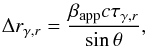 (14)where βapp is the apparent speed, c is the speed of light, θ is the viewing angle, and τγ,r is the obtained time lag. The apparent speed βapp has values ranging from 5 to 15 for its different components (Savolainen et al. 2006; Lister et al. 2013). We adopted an averaged βapp value of 7 and for the viewing angle considered θ = 9.8° (Savolainen et al. 2006).
A recent jet kinematics study suggests that the location of the 7 mm (43 GHz) VLBI core is at a distance of 4–7 pc from the jet apex. This study used core-shift measurements (Lisakov et al., in prep.). The correlation between 230 GHz and 43 GHz showed a time lag of (50 ± 10) days. This translates, by applying Eq. (14), to a relative separation of (1.7 ± 0.3) pc. Therefore, we estimate that the 230 GHz emission region is at (5.3 ± 0.3) pc from the jet apex.
3.5.2. Radio – optical correlation
Unlike the radio light-curves, the light curves at optical and IR passbands do not show any significant variability. Therefore, we do not find any significant correlation between radio and optical/IR light curves. In Fig. 11 we show the cross-correlation analysis curve between radio (230 GHz) and J passband.
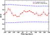 |
Fig. 11 DCF analysis curve for 230 GHz vs. J passband. The blue curve represents the 95% confidence level. |
3.5.3. Radio – X-ray correlation
The similar fractional variability amplitudes and PSD slopes for mm-radio band and X-ray light curves suggest a possible correlation. To quantify this, we applied the DCF analysis method and correlated the X-ray light curves at 14–192 keV and at 2–10 keV with the radio light-curve at 230 GHz. The DCF curves are shown in Fig. 12. The peaks of the DCF curves are above the 95% confidence level. This implies that the X-ray light curves at different bands correlate significantly with the radio light-curve at 230 GHz. We note that there is a peak at a time lag of (90 ± 10) days for the correlation curve between X-ray 14–192 keV and 230 GHz, with a coefficient of (0.7 ± 0.2), with the X-ray emission leading the radio emission. This time lag translates into 3.1 ± 0.4 pc relative distance by applying Eq. (14). For the DCF curve between X-ray 2–10 keV and 230 GHz, we measured a peak at a time lag of (10 ± 10) days, with the X-ray emission leading the radio emission and a correlation coefficient of (0.5 ± 0.3) giving a relative distance of (0.4 ± 0.4) pc. Similar results have been found for the correlation between 10–50 keV and 230 GHz, implying that the two emission regions at X-ray energies 2–10 and 10–50 keV are co-spatial.
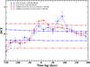 |
Fig. 12 DCF curves of X-ray at 14–192 keV vs. 230 GHz (blue) and X-ray at 2–10 keV vs. 230 GHz (red). |
3.5.4. Radio – gamma-ray correlations
We showed in Sect. 3 the apparent correlation between the mm-radio and γ-ray light curves. To quantify this, we correlated the weekly sampled γ-ray light curve with the radio light-curve at 230 GHz. Figure 13 shows the DCF curve between γ-ray and 230 GHz light curve for the entire data set. The DCF curve shows a broad and prominent peak at a time lag of 110 ± 27 days, suggesting that the γ-rays lead the radio emission by ~110 days. However, the formally calculated significance of the cross-correlation falls below 95% with regard to the whole data set. Since both radio and γ-ray light curves consist of many flares, the DCF analysis of the entire data set shows an average behaviour of different variability features. This might be due to the blending effect of the two flares ℛ1 and ℛ2 in the radio bands. However, when we restricted the DCF analysis to the time ranges of the individual flares ℛ1 and ℛ2, we found a significant correlation.
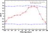 |
Fig. 13 DCF curve of γ-ray and 230 GHz light curves for the full data. The blue lines represent the 95% significance levels. |
For the first flare, the DCF curve shows a peak at 120 ± 25 days, confirming that the γ-rays lead the radio emission. For the second flare, the DCF curve has a peak at (95 ± 16) days. This suggests that the γ-ray emission is leading the radio emission and places the γ-ray emission region closer to the jet apex than the radio emission regions. Using Eq. (14), a time lag of 90 to 120 days gives an offset of Δrγ,r between 3.1 and 4.1 pc.
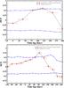 |
Fig. 14 DCF curve of γ-ray and 230 GHz during the first flare (top) and DCF curve of γ-ray and 230 GHz during the second flare (bottom). The blue lines represent the 95% confidence levels. |
3.5.5. Optical – X-ray correlation
The X-ray light curves show strong variability across the observation period, which is not the case of the optical/IR light curves. The absence of a prominent peak in the optical/IR light curves does not allow us to make any claims about a correlation between the optical/IR and X-ray bands. A formal cross-correlation analysis between the two bands does not show any peak (A.2).
3.5.6. Optical/IR – gamma-ray correlation
As shown in Fig. 1, the optical/IR light curves are not variable during the period of flaring activity in the GeV regime. The DCF analysis shows no correlation between the two bands. Similar results are obtained for the correlation between γ-ray and the optical R-band and between γ-ray and the IR J-band. This suggests different physical mechanisms and/or causally disconnected emission regions for γ-rays and optical frequencies. However, it is important to note the data gap in the optical/IR light curve during the γ-ray flares, since from an observational point of view, a simultaneous variability or delay cannot be discarded.
Although the polarisation observations in the optical band are not as well sampled as the γ-ray light curve, they are apparently correlated. For instance, we noted prominent variations in the polarisation curve during the γ-ray flaring activity period. In addition, no variation is apparent in the polarisation curve during the quiescent phase in the GeV regime (see Fig. 1). To quantify the apparent correlation, we applied the DCF analysis method. The DCF curve is shown in Fig. 15. It shows a peak at a time lag of 5 ± 5 days, which suggests a significant correlation between optical and γ-ray bands. The percentage polarisation data between MJD = 55 000 and 55 150 and between MJD = 55 400 and 55 500 have a gap. Therefore, it is essential to test this correlation using simultaneous observations.
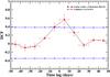 |
Fig. 15 DCF curve of γ-ray light curve and optical percentage polarisation. The blue lines represent the 95% confidence levels. |
3.5.7. X-ray – X-ray correlations
The X-ray light curves in the three different bands showed strong and similar variability behaviour during the observation time. We cross-correlated the X-ray light curve at 14–192 keV with the X-ray light curves at 2–10 keV band and 10–50 keV band. The DCF results in Fig. 16 show a correlation between the three X-ray bands. A peak close to 0 time lag is observed in the three DCF curves
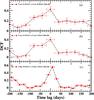 |
Fig. 16 DCF curves of the different X-ray bands: 14–192 keV vs. 10–50 keV a); 14–192 keV vs. 2–10 keV b); and 10–50 keV vs. 2−10 keV c). |
3.5.8. X-ray – γ-ray correlation
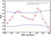 |
Fig. 17 DCF curve of γ-ray and X-Ray 2–10 keV band. The blue lines represent the 95% confidence levels. |
The source exhibits prominent flaring activity at both X-ray and γ-ray energies. The DCF curve between γ-ray and the X-ray light curve at 2–10 keV band is shown in Fig. 17. The DCF curve shows two peaks at a time lag −(50 ± 10) days and (110 ± 10) days. The positive time lag (~100 days) suggests that the γ-ray is leading the X-ray emission. The negative time lag (~−50 days) suggests that the X-ray emission is leading the γ-ray emission. The estimated time lags suggest the following two possible scenarios.
-
1.
Scenario 1: X-rays are leading the γ-ray emission with a time lag of −(50 ± 10) days, which translates into a de-projected distance of (1.7 ± 0.3) pc according to Eq. (14). The X-ray emission region is therefore closer to the jet apex than the γ-rays emission region.
-
2.
Scenario 2: gamma-rays are leading the X-ray emission with a time lag of 110 ± 10 days, corresponding to a distance of (3.8 ± 0.3) pc. The γ-ray emission region is then closer to the jet apex than the X-ray emission region i.e. X-rays are emitted from a region downstream the jet.
4. Discussion
Using the broadband variability study of the FSRQ 3C 273 observed between May 2008 and March 2012, we investigated the connection between flaring activity at GeV and lower energies. We also set constraints on the location and size of emission regions at different frequencies. The ultimate goal of the study was to provide a general physical scenario with which the observed variations of the source across several decades of frequencies can be placed in a consistent context.
4.1. Radio emission
The radio data collected between 2.6 to 350 GHz allowed us to perform a detailed study of flaring activity at radio bands. Two main outbursts (ℛ1 and ℛ2) were detected in the source during the course of our observations. We found a significant correlation between the multi-band radio data such that the flaring activity at higher radio frequencies leads those at lower frequencies. These results can be explained in the frame of the shock-in-jet model (Marscher & Gear 1985). There was no pronounced flaring activity at radio bands below 23 GHz. The fractional variability showed an increasing trend with increasing radio frequencies. The PSD slopes suggest that the lower radio frequency variations are dominated by white-noise processes. We then used the cross-correlation results between 43 and 230 GHz to locate the emission region at 230 GHz, which we found is situated at (5.3 ± 0.3) pc from the jet apex.
4.2. Optical/IR emission
Compared to the other frequencies, the observed flaring activity is significantly lower in the optical and IR regime. The estimated fractional variability amplitude is lower than 13%. In addition, the optical/IR light curves do not exhibit a significant correlation with the observed light curves at other frequencies (which might also be due to the gap in the optical data). The PSD slope results show a power-law index close to zero, which is consistent with the slope of a white-noise process. Spectral studies made on the optical/IR emission showed that this emission, particularly the excess emission at UV bands causing the blue bump, is dominated by thermal emission from the accretion disk (Shields 1978; Soldi et al. 2008). Alternatively, an X-ray source or a hot corona could contribute significantly to the optical/UV emission (Collin-Souffrin 1991; Haardt et al. 1994).
4.3. Gamma-ray emission
The source 3C 273 showed a prominent flaring activity at GeV energies between July 2009 and April 2010. Our analysis suggests a significant correlation between the γ-rays and the 230 GHz light curve, with a time lag of (110 ± 27) days, which translates into a relative separation between γ-ray and 230 GHz emission region of around (3.8 ± 0.9) pc. The radio correlation between 43 and 230 GHz sets the location of the 230 GHz emission region at a distance of (5.3 ± 0.3) pc from the jet apex. This places the γ-ray emission region at a distance of (1.2 ± 0.9) pc from the jet apex. This result agrees with the result found in Rani et al. (2013b), who constrained the γ-ray emission region to <1.6 pc from the jet apex.
The fractional variability amplitude in the radio bands is around 40%, whereas the γ-ray light curves showed a fractional variability amplitude of around 100%. The PSD slope at mm-radio bands and γ-ray energies are similar, however, and are consistent with the slopes of a red-noise process. Moreover, the longest variability timescale at high radio frequencies is very similar to that at γ-ray energies, which implies a similar size of the emission region for the two energy ranges. The fastest variability timescale for the γ-ray frequency is 1.1 h (Rani et al. 2013b), suggesting several very compact emission regions at γ-ray energy bands, as is expected from the multi-zone emission model suggested by Marscher (2014).
The spectral changes reported in Rani et al. (2013b) suggest an external Compton mechanism with seed photons from the broad-line region (BLR). The optical polarisation has significantly increased during the γ-ray flaring activity, which suggests a possible correlation between the γ-rays and the optical polarisation. This indicates that the non-thermal emission component and the γ-ray emission are linked. A detailed broadband spectral energy distribution (SED) modelling will shed more light on SSC (synchrotron self-Compton) and EC (external-Compton) contribution.
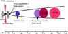 |
Fig. 18 Sketch representing the location of the emission regions at different frequencies. |
4.4. X-ray emission
In comparison to a brief episode of flaring activity (July 2009 to April 2010) followed by a quiescence phase at radio and γ-ray frequencies, the X-ray regime was dominated by episodes of repeated variability. The DCF curve between γ-rays and X-rays shows two time lags, one being negative with −(50 ± 10) days, and another being positive with a time lag of 110 ± 10 days. The DCF analysis suggests that two possible components are responsible for the X-ray emission. The negative time lag suggests the X-ray emission is leading the γ-ray emission and is located at a distance of 0.1 to 0.5 pc from the jet apex. The positive time lag suggests that the γ-ray emission is leading the X-ray emission with a corresponding separation distance of (3.8 ± 0.3) pc. This component could be emitted from the jet through inverse-Compton processes. An independent study of the X-ray spectrum also suggests that there are two components: a component emitted from a hot corona or reflected off an accretion disk, which accounts for the weak iron line found in the X-ray spectrum at 3–78 keV, and a second component most likely emitted from the jet, which starts to dominate at 30–40 keV (Madsen et al. 2015).
The two-component scenario for the X-ray emission was also confirmed by an X-ray vs. radio correlation analysis. We noted similar fractional variability amplitudes for the three X-ray bands and the mm-radio bands. The PSD slopes are also similar for the mm-radio bands and X-ray at 2–10 keV and 10–50 keV. The SF analysis showed a quasi-periodic variability for both X-ray and mm-radio light curves. The correlation analysis suggests a time lag of 90 ± 10 days between 14–192 keV X-ray light curve and 230 GHz light curve, which translates into 3.1 ± 0.4 pc and places the location of the X-ray emission region at 0.5 to 2 pc from the jet apex. The DCF curve between X-rays at 2–10 keV and 230 GHz shows a time lag of (10 ± 10) days, which gives a relative distance between the X-ray and radio emission regions of (0.4 ± 0.4) pc. This provides an estimate of the location of 2–10 keV X-ray emission at 4.7 ± 0.4 pc from the jet apex. We obtained similar results for the intensity variations at 10–50 keV X-ray band.
The longest variability timescale for the X-ray light curves is ~230 days. To estimate the size of the emission region, we applied (Rani et al. 2013b) 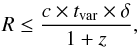 (15)where R is the size of the emission region, tvar is the shortest variability timescale, c is the speed of light, δ is the Doppler factor of the source for which we used a value of 7 (Savolainen et al. 2006), and z is the redshift of the source. For a variability timescale of ~230 days, we obtained an emission region with a size of ~1.2 pc. The size of this emission region is much larger than the size of the corona, which was suggested to be around 20–30 RS (0.013–0.02 pc) (Reis & Miller 2013), where RS = 6.4 × 10⁻⁴ pc is the Schwarzschild radius of the black hole, where the mass of SMBH of 3C 273 is around 6.6 × 10⁹ M⊙ (Paltani & Türler 2005). However, we noted that for the X-ray light curves used in this study, the shortest variability timescale is ~5–10 days. This translates into a size of 0.025–0.05 pc, which is similar to the size of the corona. This implies that the long-term variability probably comes from the jet, whereas the faster variability seems to be originating closer to the black hole.
4.5. Broadband correlation alignment
The statistical analysis we presented suggests a causal connection between the observed broadband flaring activity in the source. The proposed scenario is presented in Fig. 18, where we marked the location of different emission regions. A moving shock or disturbance propagating downstream of the jet might first produce the γ-ray flares at a distance of ~1.2 pc and later brighten the emission region at mm-radio bands. The mm-radio flares lead those at cm-radio bands. Delayed emission at cm-radio bands is a clear indication of opacity effects that are due to synchrotron self-absorption. Our analysis suggests that two possible components are responsible for the X-ray emission. One component of the X-ray emission most likely comes from the hot corona or jet apex. The second X-ray component seems to have non-thermal origin, that is, it is produced through inverse-Compton scattering of radio synchrotron photons at a distance of ~4.7 pc from the jet apex. Observations at optical/IR regime suggest a prominent thermal dominance from the accretion disk or/and from the BLR region.
5. Conclusion
We presented the results of our broadband variability study of the FSRQ 3C 273 observed between May 2008 and March 2012. A detailed statistical analysis was performed to constrain the location of the emission region at different energy bands and to explore the connection between the broadband flaring activity.
The source went through a series of rapid flares at the γ-rays, which was accompanied by flaring activity at other energies. We studied the broadband variability behaviour of 3C 273 by comparing the general behaviour and the properties of the light curves at different energy bands. Except for the light curves at cm-radio and optical/IR frequencies, the observed broadband variations were found to be consistent with red-noise processes. The absence of a pronounced flaring activity at cm-radio bands might be due to synchrotron self-absorption, and at optical/IR bands the reason might be the dominance of thermal emission. The optical/IR emission seems to be dominated by thermal emission from the disk and/or the BLR.
At radio bands, the fractional variability amplitude increases with increasing frequency, while the variability timescale decreases. This implies that we probe more compact emission regions at higher frequencies. In addition, the variability timescales were found to be very similar at different regimes. The estimated fractional variability seems to follow a double-hump structure as a function of frequency, which suggests that the strongest variations are seen for the highest energy photons.
The evolution of radio flares are well explained in the frame of the shock-in-jet model. From the correlation analysis, we found that the 230 GHz radio flares are emitted at a distance of about 5.3 pc from the jet apex. The γ-ray energies are emitted from a compact region at a distance ~1.2 pc from the jet apex through IC processes. Two components seem to be responsible for the X-ray emission. The first component is located within a distance of 0.1–0.5 pc from the jet apex and is most likely emitted either by the corona or regions closer to the jet apex. The second component responsible for X-ray emission is located at a distance of ~4.7 pc and is produced through up-scattering of radio synchrotron photons through IC processes. A broadband spectral energy density analysis can provide better constraints on the different emission mechanisms that take place in the jet.
DCF peaks above the 95% confidence level are considered to be significant.
Acknowledgments
C.C. was supported for this research through a stipend from the International Max Planck Research School (IMPRS) for Astronomy and Astrophysics at the Universities of Bonn and Cologne. The authors would like to thank Dimitris Emmanoulopoulos, Sam Connolly, and Walter Max-Moerbeck for useful discussions on statistical analysis and for their suggestions and comments on the paper draft. This research is partly based on observations with the 100 m telescope of the MPIfR (Max-Planck-Institut für Radioastronomie) at Effelsberg. The optical/IR observations are provided by the Yale Fermi/SMARTS project. Data from the Steward Observatory spectropolarimetric monitoring project were used. This program is supported by Fermi Guest Investigator grants NNX08AW56G, NNX09AU10G, NNX12AO93G, and NNX15AU81G. The Submillimeter Array is a joint project between the Smithsonian Astrophysical Observatory and the Academia Sinica Institute of Astronomy and Astrophysics and is funded by the Smithsonian Institution and the Academia Sinica. This research is partly based on observations carried out with the IRAM 30 m telescope. IRAM is supported by INSU/CNRS (France), MPG (Germany) and IGN (Spain).
References
- Abdo, A. A., Ackermann, M., Agudo, I., et al. 2010, ApJ, 716, 30 [NASA ADS] [CrossRef] [Google Scholar]
- Abramowitz, M., & Stegun, I. 1964, Handbook of Mathematical Functions, Applied Mathematics Series (New York: Dover Publications), 55 [Google Scholar]
- Angelakis, E., Fuhrmann, L., Marchili, N., Krichbaum, T. P., & Zensus, J. A. 2008, Mem. Soc. Astron. It., 79, 1042 [NASA ADS] [Google Scholar]
- Beaklini, P. P. B., & Abraham, Z. 2014, MNRAS, 437, 489 [NASA ADS] [CrossRef] [Google Scholar]
- Bonning, E., Urry, C. M., Bailyn, C., et al. 2012, ApJ, 756, 13 [NASA ADS] [CrossRef] [Google Scholar]
- Chatterjee, R., Bailyn, C. D., Bonning, E. W., et al. 2012, ApJ, 749, 191 [NASA ADS] [CrossRef] [Google Scholar]
- Chernyakova, M., Neronov, A., Courvoisier, T. J.-L., et al. 2007, A&A, 465, 147 [NASA ADS] [CrossRef] [EDP Sciences] [Google Scholar]
- Collin-Souffrin, S. 1991, A&A, 249, 344 [NASA ADS] [Google Scholar]
- Connolly, S. D. 2015, ArXiv e-prints [arXiv:1503.06676] [Google Scholar]
- Edelson, R. A., & Krolik, J. H. 1988, ApJ, 333, 646 [NASA ADS] [CrossRef] [Google Scholar]
- Emmanoulopoulos, D., McHardy, I. M., & Uttley, P. 2010, MNRAS, 404, 931 [NASA ADS] [CrossRef] [Google Scholar]
- Emmanoulopoulos, D., McHardy, I. M., & Papadakis, I. E. 2013, MNRAS, 433, 907 [NASA ADS] [CrossRef] [Google Scholar]
- Fromm, C. M., Perucho, M., Ros, E., et al. 2011, A&A, 531, A95 [NASA ADS] [CrossRef] [EDP Sciences] [Google Scholar]
- Fuhrmann, L., Zensus, J. A., Krichbaum, T. P., Angelakis, E., & Readhead, A. C. S. 2007, in The First GLAST Symposium, eds. S. Ritz, P. Michelson, & C. A. Meegan, AIP Conf. Proc., 921, 249 [Google Scholar]
- Fuhrmann, L., Larsson, S., Chiang, J., et al. 2014, MNRAS, 441, 1899 [NASA ADS] [CrossRef] [Google Scholar]
- Geweke, J., & Porter-Hudak, S. 1989, J. Time Series Analysis, 4, 221 [Google Scholar]
- Grandi, P., & Palumbo, G. G. C. 2004, Science, 306, 998 [NASA ADS] [CrossRef] [Google Scholar]
- Gurwell, M. A., Peck, A. B., Hostler, S. R., Darrah, M. R., & Katz, C. A. 2007, in From Z-Machines to ALMA: (Sub)Millimeter Spectroscopy of Galaxies, eds. A. J. Baker, J. Glenn, A. I. Harris, J. G. Mangum, & M. S. Yun, ASP Conf. Ser., 375, 234 [Google Scholar]
- Haardt, F., Maraschi, L., & Ghisellini, G. 1994, ApJ, 432, L95 [NASA ADS] [CrossRef] [Google Scholar]
- Hartman, R. C., Bertsch, D. L., Fichtel, C. E., et al. 1992, in NASA Conf. Publ. 3137, eds. C. R. Shrader, N. Gehrels, & B. Dennis [Google Scholar]
- Ikejiri, Y., Uemura, M., Sasada, M., et al. 2011, PASJ, 63, 639 [NASA ADS] [Google Scholar]
- Jahoda, K. 1994, BAAS, 26, 894 [Google Scholar]
- Jorstad, S., Marscher, A., Smith, P., et al. 2012, Int. J. Mod. Phys. Conf. Ser., 8, 356 [CrossRef] [Google Scholar]
- Kudryavtseva, N. A., Gabuzda, D. C., Aller, M. F., & Aller, H. D. 2011, MNRAS, 415, 1631 [NASA ADS] [CrossRef] [Google Scholar]
- Lister, M. L., Aller, M. F., Aller, H. D., et al. 2013, AJ, 146, 120 [NASA ADS] [CrossRef] [Google Scholar]
- Liu, W.-P., & Shen, Z.-Q. 2009, RA&A, 9, 520 [Google Scholar]
- Lobanov, A. P. 1998, A&A, 330, 79 [NASA ADS] [Google Scholar]
- Madsen, K. K., Fürst, F., Walton, D. J., et al. 2015, ApJ, 812, 14 [NASA ADS] [CrossRef] [Google Scholar]
- Marscher, A. P. 2014, ApJ, 780, 87 [NASA ADS] [CrossRef] [Google Scholar]
- Marscher, A. P., & Gear, W. K. 1985, ApJ, 298, 114 [NASA ADS] [CrossRef] [Google Scholar]
- Max-Moerbeck, W., Hovatta, T., Richards, J. L., et al. 2014, MNRAS, 445, 428 [NASA ADS] [CrossRef] [Google Scholar]
- McHardy, I., Lawson, A., Newsam, A., et al. 1999, MNRAS, 310, 571 [NASA ADS] [CrossRef] [Google Scholar]
- McHardy, I., Lawson, A., Newsam, A., et al. 2007, MNRAS, 375, 1521 [NASA ADS] [CrossRef] [Google Scholar]
- Paltani, S., & Türler, M. 2005, A&A, 435, 811 [NASA ADS] [CrossRef] [EDP Sciences] [Google Scholar]
- Paltani, S., Courvoisier, T. J.-L., & Walter, R. 1998, A&A, 340, 47 [NASA ADS] [Google Scholar]
- Papadakis, I. E., & Lawrence, A. 1993, MNRAS, 261, 612 [NASA ADS] [CrossRef] [Google Scholar]
- Ramakrishnan, V., Hovatta, T., Nieppola, E., et al. 2015, MNRAS, 452, 1280 [CrossRef] [Google Scholar]
- Rani, B., Krichbaum, T. P., Fuhrmann, L., et al. 2013a, A&A, 552, A11 [NASA ADS] [CrossRef] [EDP Sciences] [Google Scholar]
- Rani, B., Lott, B., Krichbaum, T. P., Fuhrmann, L., & Zensus, J. A. 2013b, A&A, 557, A71 [NASA ADS] [CrossRef] [EDP Sciences] [Google Scholar]
- Rani, B., Wiita, P. J., & Gupta, A. C. 2009, ApJ, 696, 2170 [NASA ADS] [CrossRef] [Google Scholar]
- Reis, R. C., & Miller, J. M. 2013, ApJ, 769, L7 [Google Scholar]
- Robson, E. I., Litchfield, S. J., Gear, W. K., et al. 1993, MNRAS, 262, 249 [NASA ADS] [CrossRef] [Google Scholar]
- Ross, R. R., & Fabian, A. C. 1993, MNRAS, 261, 74 [NASA ADS] [CrossRef] [Google Scholar]
- Savolainen, T., Wiik, K., Valtaoja, E., & Tornikoski, M. 2006, A&A, 446, 71 [NASA ADS] [CrossRef] [EDP Sciences] [Google Scholar]
- Schmidt, M. 1963, Nature, 197, 1040 [NASA ADS] [CrossRef] [Google Scholar]
- Shields, G. A. 1978, Nature, 272, 706 [NASA ADS] [CrossRef] [Google Scholar]
- Simonetti, J. H., Cordes, J. M., & Heeschen, D. S. 1985, ApJ, 296, 46 [NASA ADS] [CrossRef] [Google Scholar]
- Smith, P. S., Montiel, E., Rightley, S., et al. 2009, Fermi Symp., eConf Proceedings C091122 [arXiv:0912.3621] [Google Scholar]
- Sokolov, A., & Marscher, A. P. 2005, ApJ, 629, 52 [NASA ADS] [CrossRef] [Google Scholar]
- Soldi, S., Türler, M., Paltani, S., et al. 2008, A&A, 486, 411 [NASA ADS] [CrossRef] [EDP Sciences] [Google Scholar]
- Stroh, M. C., & Falcone, A. D. 2013, ApJS, 207, 28 [NASA ADS] [CrossRef] [Google Scholar]
- Timmer, J., & Koenig, M. 1995, A&A, 300, 707 [NASA ADS] [Google Scholar]
- Türler, M., Courvoisier, T. J.-L., & Paltani, S. 1999, A&A, 349, 45 [NASA ADS] [Google Scholar]
- Uchiyama, Y., Urry, C. M., Cheung, C. C., et al. 2006, ApJ, 648, 910 [NASA ADS] [CrossRef] [Google Scholar]
- Uemura, M., & Kanata Team. 2009, in The Eighth Pacific Rim Conference on Stellar Astrophysics: A Tribute to Kam-Ching Leung, eds. B. Soonthornthum, S. Komonjinda, K. S. Cheng, & K. C. Leung, ASP Conf. Ser., 404, 69 [Google Scholar]
- Uttley, P., McHardy, I. M., & Papadakis, I. E. 2002, MNRAS, 332, 231 [NASA ADS] [CrossRef] [Google Scholar]
- Valtaoja, L., Takalo, L. O., Sillanpaa, A., et al. 1991, AJ, 102, 1946 [NASA ADS] [CrossRef] [Google Scholar]
- Vaughan, S. 2005, A&A, 431, 391 [NASA ADS] [CrossRef] [EDP Sciences] [Google Scholar]
- Vaughan, S., Edelson, R., Warwick, R. S., & Uttley, P. 2003, MNRAS, 345, 1271 [NASA ADS] [CrossRef] [Google Scholar]
- Walter, R., & Courvoisier, T. J.-L. 1992, A&A, 258, 255 [NASA ADS] [Google Scholar]
Appendix A: Structure function, cross-correlation analysis, and PSD plots
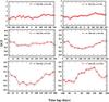 |
Fig. A.1 Cross-correlation analysis curves at radio frequencies (230 GHz vs. 2.6, 5, 8, 10, 15, and 23 GHz). |
 |
Fig. A.2 Cross-correlation analysis curves. |
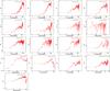 |
Fig. A.3 Structure function curves at radio (2.6 to 350 GHz bands), IR (J-band), optical (R and V-bands), X-ray (10–50 keV and 14–192 keV), and γ-ray frequencies. |
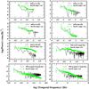 |
Fig. A.4 PSD curves at radio (2.6 to 350 GHz), IR (J-band), optical (R and V-bands), X-ray, and γ-ray frequencies. |
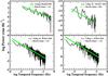 |
Fig. A.5 PSD curves at X-ray and γ-ray frequencies. |
All Tables
All Figures
|
Fig. 1 Broadband light curves of 3C 273: a) weekly (turquoise circles) and monthly (blue circles) averaged γ-ray light curves; b) 14–192 keV band (cyan), the 10–50 keV band (indigo) and the 2–10 keV band (magenta) X-ray light curves; c) optical (V and R passbands) and IR (J passband) light curves; d) optical percentage polarisation curve; and e) radio flux density curves at 230 GHz (in black) and 350 GHz (in green) bands. |
| In the text | |
|
Fig. 2 X-ray light curves of 3C 273 at 14−192 keVa), 10−50 keVb), and 2−10 keVc). |
| In the text | |
|
Fig. 3 Radio (cm to mm) band light curves of 3C 273. Different colours represent different frequencies, from 2.6 GHz to 350 GHz (from top to bottom). |
| In the text | |
|
Fig. 4 Fractional variability amplitude plotted as a function of frequency. The red (black) point shows the fractional variability amplitude of the monthly (weekly) averaged γ-ray light curve. |
| In the text | |
|
Fig. 5 Structure function at the 230 GHz radio band (top) and 2–10 keV X-ray band (bottom). |
| In the text | |
|
Fig. 6 Variability timescales plotted as a function of frequency (Hz). |
| In the text | |
|
Fig. 7 Best-fitting average power spectrum (in green) superimposed on the raw power spectrum at the 230 GHz radio band (in black). |
| In the text | |
|
Fig. 8 Best-fit power-law index plotted as a function of the frequency. |
| In the text | |
|
Fig. 9 Cross-correlation functions of the 230 GHz data vs. the data at 23, 32, 43, 86, 142, and 350 GHz. |
| In the text | |
|
Fig. 10 Time lag relative to the curve at 230 GHz plotted as a function of radio frequencies (in blue). The green curve represents the best power-law fit of the data points, with a slope of kr = 1.12 ± 0.46. The grey shaded area represents the error interval on the fit. |
| In the text | |
|
Fig. 11 DCF analysis curve for 230 GHz vs. J passband. The blue curve represents the 95% confidence level. |
| In the text | |
|
Fig. 12 DCF curves of X-ray at 14–192 keV vs. 230 GHz (blue) and X-ray at 2–10 keV vs. 230 GHz (red). |
| In the text | |
|
Fig. 13 DCF curve of γ-ray and 230 GHz light curves for the full data. The blue lines represent the 95% significance levels. |
| In the text | |
|
Fig. 14 DCF curve of γ-ray and 230 GHz during the first flare (top) and DCF curve of γ-ray and 230 GHz during the second flare (bottom). The blue lines represent the 95% confidence levels. |
| In the text | |
|
Fig. 15 DCF curve of γ-ray light curve and optical percentage polarisation. The blue lines represent the 95% confidence levels. |
| In the text | |
|
Fig. 16 DCF curves of the different X-ray bands: 14–192 keV vs. 10–50 keV a); 14–192 keV vs. 2–10 keV b); and 10–50 keV vs. 2−10 keV c). |
| In the text | |
|
Fig. 17 DCF curve of γ-ray and X-Ray 2–10 keV band. The blue lines represent the 95% confidence levels. |
| In the text | |
|
Fig. 18 Sketch representing the location of the emission regions at different frequencies. |
| In the text | |
|
Fig. A.1 Cross-correlation analysis curves at radio frequencies (230 GHz vs. 2.6, 5, 8, 10, 15, and 23 GHz). |
| In the text | |
|
Fig. A.2 Cross-correlation analysis curves. |
| In the text | |
|
Fig. A.3 Structure function curves at radio (2.6 to 350 GHz bands), IR (J-band), optical (R and V-bands), X-ray (10–50 keV and 14–192 keV), and γ-ray frequencies. |
| In the text | |
|
Fig. A.4 PSD curves at radio (2.6 to 350 GHz), IR (J-band), optical (R and V-bands), X-ray, and γ-ray frequencies. |
| In the text | |
|
Fig. A.5 PSD curves at X-ray and γ-ray frequencies. |
| In the text | |
Current usage metrics show cumulative count of Article Views (full-text article views including HTML views, PDF and ePub downloads, according to the available data) and Abstracts Views on Vision4Press platform.
Data correspond to usage on the plateform after 2015. The current usage metrics is available 48-96 hours after online publication and is updated daily on week days.
Initial download of the metrics may take a while.