| Issue |
A&A
Volume 590, June 2016
|
|
|---|---|---|
| Article Number | A82 | |
| Number of page(s) | 8 | |
| Section | Extragalactic astronomy | |
| DOI | https://doi.org/10.1051/0004-6361/201628326 | |
| Published online | 16 May 2016 | |
The dependence of gamma-ray burst X-ray column densities on the model for Galactic hydrogen
1
Department of Physics G. OcchialiniUniversity of
Milano-Bicocca, Piazza della
Scienza 3, 20126
Milano, Italy
e-mail:
This email address is being protected from spambots. You need JavaScript enabled to view it.
2
INAF–Osservatorio Astronomico di Brera,
via Bianchi 46, 23807 Merate
( LC), Italy
e-mail:
This email address is being protected from spambots. You need JavaScript enabled to view it.
3
INAF, IASF Milano, via E. Bassini 15, 20133
Milano,
Italy
Received: 17 February 2016
Accepted: 25 March 2016
Abstract
We study the X-ray absorption of a complete sample of 99 bright Swift gamma-ray bursts (GRBs). In recent years, a strong correlation has been found between the intrinsic X-ray absorbing column density (NH(z)) and the redshift. This absorption excess in high-z GRBs is now thought to be due to the overlooked contribution of the absorption along the intergalactic medium (IGM), by means of both intervening objects and the diffuse warm-hot intergalactic medium along the line of sight. In this work we neglect the absorption along the IGM, because our purpose is to study the eventual effect of a radical change in the Galactic absorption model on the NH(z) distribution. Therefore, we derive the intrinsic absorbing column densities using two different Galactic absorption models: the Leiden Argentine Bonn HI survey and the more recent model that includes molecular hydrogen. We find that if, on the one hand, the new Galactic model considerably affects the single column density values, on the other hand, there is no drastic change in the distribution as a whole. It becomes clear that the contribution of Galactic column densities alone, no matter how improved, is not sufficient to change the observed general trend and it has to be considered as a second order correction. The cosmological increase of NH(z) as a function of redshift persists and, to explain the observed distribution, it is necessary to include the contribution of both the diffuse intergalactic medium and the intervening systems along the line of sight of the GRBs.
Key words: gamma-ray burst: general / X-rays: general
© ESO, 2016
1. Introduction
Long gamma-ray bursts (LGRBs) are associated with type Ibc supernova explosions (Woosley & Bloom 2006) and observed in galactic regions with high star formation rate (Fruchter et al. 2006): this enables us to infer that LGRBs have massive stars as progenitors. Moreover, their circumburst medium is thought to be denser than the typical star formation regions, as we can see from the high absorbing column density values measured in X-rays (Galama & Wijers 2001; Stratta et al. 2004; Gendre et al. 2006). Both metals in the circumburst medium and within the whole host galaxy may contribute to the intrinsic column density NH(z). In addition, X-ray absorption occurs within our Galaxy (parametrized by NH(Gal)) and along the line of sight owing to the intergalactic medium (IGM). This occurs by means of a warm-hot diffuse medium that pervades it or, mainly, by means of compact discrete intervening systems (galactic halos, galaxy groups) casually placed along the line of sight of the GRB (Behar et al. 2011; Eitan & Behar 2013; Starling et al. 2013; Campana et al. 2015, and references therein).
Campana et al. (2012, hereafter C12) worked out a redshift distribution of the intrinsic column density of a complete sample of 58 Swift LGRBs, assuming that the absorption along the IGM is negligible. An increasing trend of NH(z) emerged with the redshift of the GRB, indicating a lack of non-absorbed GRBs at high redshift or, alternatively, an absorption excess in high-z GRBs. The sample in C12, named BAT6 (Salvaterra et al. 2012), has been selected above a specific threshold of the gamma peak flux and has a high completeness in redshift, which is fundamental not only to exclude the hypothesis that the NH(z)−z correlation is due to observative biases, but also to provide the real intrinsic column density values calculated at the GRB redshift, taking account of the scaling cosmological factor ~(1 + z)2.4 (see Campana et al. 2014). Recently, it has been shown that a model, which includes the (previously overlooked) contributions of both the intervening objects and the diffuse warm-hot intergalactic medium along the line of sight, could explain qualitatively and quantitatively the observed NH(z) distribution (Campana et al. 2015; see also Behar et al. 2011; Eitan & Behar 2013; Starling et al. 2013).
We now derive the intrinsic column densities while still neglecting the contribution along the IGM (then allocating all the absorption in excess to the host galaxy), because our purpose is to study the eventual effect on the NH(z) distribution of a radical change in the Galactic absorption model. We keep the Galactic component fixed, using the Leiden Argentine Bonn (LAB) HI survey (Kalberla et al. 2005, which is largely adopted by previous literature, including C12) to verify the NH(z)−z correlation and, in addition, we consider the new Galactic absorption model introduced by Willingale et al. (2013, hereafter W13). This new model completes the HI distribution of the LAB survey, obtained in radio, adding the contribution of the molecular hydrogen that was extracted from the IR dust absorption in our Galaxy. Therefore, this model reports generally greater values than the LAB survey and, consequently, the new intrinsic column density values are expected to be smaller. Moreover, we derive our results using an extended complete sample of 99 Swift LGRBs, which is called BAT6ext and updated to GRB 140703A with the bursts detected by Swift that have satisfied the same selection criteria since the construction of the BAT6 (Pescalli et al. 2016). With this extension, we enlarge our sample from 58 to 99 LGRBs, but we slightly lose redshift completeness from 95% to 82%.
2. X-ray absorbing column density distribution
The intrinsic column densities were computed from GRBs X-ray afterglow spectral fits using the UK Swift Science Data Centre spectra repository, which provides Swift/XRT data suitable for scientific analysis (Evans et al. 2009). All the results, listed in Table A.1, are obtained by selecting a specific time interval when there are no strong spectral variations. This is obtained by strictly selecting time intervals when the hardness ratio (between counts in the 1.5−10 keV and in the 0.3−1.5 keV bands) is constant. For an afterglow spectrum modelled as a power law, this condition ensures that no strong spectral changes are occurring. This is particularly important because any curvature estimate of the X-ray spectrum would reverberate into the column density, which in turn would produce biased values (Butler & Kocevski 2007).
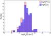 |
Fig. 1 Intrinsic X-ray absorbing column density distributions of the BAT6ext sample. The dotted (red) histogram is related to the |
Each spectrum was then fitted by a power law that was absorbed by both a Galactic component, held fixed, and an intrinsic component at the redshift of the GRB, which were modelled with TBABS and ZTBABS, respectively, within XSPEC (version 12.9.0). We note that the results in C12 were obtained by using different models, namely PHABS and ZPHABS (the Leicester Swift automatic spectral analysis tool adopted the TBabs models only in 20141). Therefore, the intrinsic column density values of the BAT6 GRBs, which are used by both works, are slightly different. Abundances from Wilms et al. (2000) and cross-sections from Verner et al. (1996) were used. Table A.1 shows the intrinsic column density values obtained using the Galactic absorption models provided by both LAB and W13 surveys, the latter being labelled as new. In addition, for the 18 GRBs of the BAT6ext sample that have no spectroscopic redshift, we fixed z to be zero and, consequently, the intrinsic column densities have to be considered as lower limits.
The two NH(z) distributions are shown in Fig. 1 and can be described by a Gaussian, with a mean value of log (NH/ cm-2) = 21.93 ± 0.54 and log (NH/ cm-2) = 21.84 ± 0.61, for the LAB survey and the W13 Galactic model, respectively. The latter mean value is only slightly smaller but fully consistent with the former. This probably indicates that the change in the Galactic column densities plays a minor role in shaping the intrinsic column density distribution. Both values are consistent with the distribution of column densities reported in C12, which is log (NH/ cm-2) = 21.7 ± 0.5. This indicates that the impact of different Swift/XRT response matrices2 and absorption model (PHABS was adopted) again do not play a major role in the NH(z) distribution.
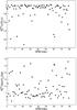 |
Fig. 2 Top panel: ratio between new and old intrinsic column densities, as a function of an index representing the 81 GRBs of Table A.1 with a measure of redshift. Bottom panel: the comparable distribution of the ratio between the new (W13) and the old (LAB) Galactic column densities is shown. |
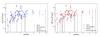 |
Fig. 3 Intrinsic X-ray column density distribution as a function of redshift for both Galactic models. The panel on the left shows the NH(z) distribution obtained with the LAB survey. We note that the 41 GRBs of the extended sample, shown in a lighter colour with respect to the (blue) dots of the BAT6 sample, do not affect the increasing trend that came out in C12. The panel on the right reports the |
In Fig. 2, the ratio between the new and the old intrinsic column densities is reported for all GRBs of Table A.1. While it is clear that every new single value shows a decrease (with a maximum of a factor ~5), most of them are only marginally affected by the different Galactic model that was used. This is because, as we expected, the ratio between the new and the old Galactic column densities is, in almost all cases, just slightly greater than 1 (see bottom panel of Fig. 2).
The redshift distributions of the X-ray intrinsic column density are shown in Fig. 3. The increasing trend of NH(z) with redshift is still evident, not only in the distribution obtained with the LAB Galactic model, but also in the distribution obtained with the new W13 Galactic model. This states that, even if the W13 model changes single values, the whole NH(z) distribution follows the same increasing trend found in previous works. Furthermore, we note that the supplementary 41 GRBs of the extended BAT6 sample are distributed evenly among the other column densities, with no influence on the observed pattern. Hence, it seems that neither a radical improvement of the Galactic model nor an extension of the sample affect the observed general trend in the NH(z) distribution. This suggests that those should be considered as second order corrections.
2.1. Monte Carlo simulations and K-S test
It seems that the uniform trend of absorbing column densities at low redshift does not persist at high redshift. To see if there is a real difference, whereby the increasing trend could not be attributed to statistical fluctuations, we cut the sample at z = 1 (where the distribution bends) and carried out a Kolmogorov-Smirnov test on the two NH(z) subsamples. Monte Carlo simulations have been used to provide 10 000 NH(z) values for each GRB, extracted from a Gaussian distribution that peaked at the intrinsic column density values listed in Table A.1 (and with a width of 1σ). Furthermore, for the 18 GRBs of the BAT6ext sample, which do not have a redshift measure, we also simulated z, extracting the values from the redshift probability density function that was obtained from the other 81 GRBs of the sample. We then scaled the corresponding NH(z = 0), previously simulated, with the factor (1 + z)2.4. For each iteration, we computed the K-S test and obtained a distribution of (log) probabilities, with mean values log P = −5.02 ± 0.95 and log P = −4.68 ± 0.99, for the intrinsic column densities obtained with the LAB survey and with the W13 Galactic model, respectively. These values are extremely low, and, as we can see in Fig. 4, even the tails of the two distributions never reach a 1% probability.
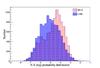 |
Fig. 4 Kolmogorov-Smirnov (log) probability distributions. The dotted (red) histogram relates to the |
In addition, a much more brutal technique has been used to include those 18 GRBs in the simulations. We fixed z to be 1 and we simulated the NH(z) values, first attributing all the z = 1 GRBs to the subsample of GRBs with redshift under z = 1, and then to the other subsample. Then, the K-S test was carried out. This obtained, in the former case, mean values log P = −3.02 ± 0.52 and log P = −2.60 ± 0.44 (for the values obtained with the LAB survey and the W13 model, respectively). In the latter case, mean values log P = −3.44 ± 0.69 and log P = −3.42 ± 0.66 were obtained (for LAB survey and W13 model, respectively). This technique was seen as useful proof, demonstrating that even in the most extreme cases, i.e., allocating all the GRBs around the bending redshift, the difference between the two sub-distributions does not seem to be due to adverse statistics.
In all these instances, the probability of having the two subsamples descend from the same parent distribution is extremely low. This indicates that there is a real difference between the two sub-distributions of column densities NH(z) in excess of the Galactic value. Therefore the increasing trend of the intrinsic column density as a function of redshift can not be due to statistical fluctuations. With this test, we can not attribute all the absorption in excess to the host galaxy, which leads us to suppose that every single value of these NH(z) distributions actually includes a contribution that clearly increases with the redshift. One possibility to account for this is to invoke the overlooked component of the absorption along the IGM, which obviously increases with the distance of the GRB (Behar et al. 2011; Campana et al. 2015). Alternatively, one would have to postulate that the GRB environment gets denser with redshift.
In addition, we performed a K-S test to show that GRBs with an upper limit in the measure of NH(z) are uniformly distributed in redshift. This is important for assuring that the increasing trend of NH(z) with the redshift is not due to an incapability of measuring low NH at high z. In our sample, a measure of NH(z) is provided essentially for almost all GRBs, but the eventual presence of most of the upper limit measures at high redshift could give rise to some objections. Hence, we separated into two subsamples the redshift of GRBs with a measure of NH(z), and the redshift of GRBs with an upper limit (denoted with a ↓ in Table A.1). We then computed a K-S test for each iteration of the Monte Carlo simulation. We obtained mean probabilities of P = 30 ± 8% and P = 25 ± 9% (for measures obtained with the LAB Galactic model and W13, respectively), which indicates that the two sets of redshift originate from the same parent distribution.
2.2. Correlations of NH(z)
We already highlighted the fact that the only selection effect of our sample is the peak flux limit and that it is also highly complete in redshift, which means we can compare the rest frame physical properties of GRBs in an unbiased way. In this work, we analyzed the intrinsic X-ray absorbing column density redshift distribution. Moreover, the rest-frame peak energy  and the bolometric equivalent isotropic luminosity Liso have been computed by Pescalli et al. (2016) for each GRB of the BAT6ext with a redshift measure.
We now want to study the eventual correlation between NH(z) and these quantities3. However, given that the sample was selected above a peak flux threshold, and, primarily, Liso have a tight correlation with redshift. This is due to the fact that, for a flux-limited sample, the only sources detected out to great distances are necessarily powerful (see Blundell et al. 1999). However, we do not expect any correlation between NH(z) and luminosities (or energies), but, since all these quantities correlate with z, we must take the precaution of doing a correlation test that excludes the dependence on redshift. Indeed, the spurious correlation between NH(z) and (Liso) can be avoided by using a partial correlation analysis. First, we computed the Spearman rank correlation coefficient r (Spearman 1904) for each case, namely r12, r13, and r23, where 1, 2 represent NH(z) and (Liso), respectively, and 3 is z. Then, we obtained the correlation coefficient between 1 and 2, excluding the redshift bias: 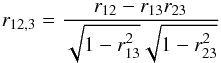 (1)(see Kendall & Stuart 1979, Chap. 27; Padovani 1992).
From the Spearman rank coefficient one can derive the associated probability value to calculate the significance of the correlation. The coefficient between NH(z) ( ) and is r12,3 = 0.056 (0.093) and the related probability is P = 62% (41%), while the correlation coefficient between NH(z) () and Liso is r12,3 = 0.052 (0.075), with probability P = 65% (51%). Hence, the results of the partial correlation analysis state that NH(z) does not correlate with and Liso. Being NH(z) connected to the distribution of matter along the line of sight and and Liso to the GRB prompt emission, this result is not surprising.
Furthermore, our data can be used to test the anticorrelation between the X-ray absorbing column density in excess of the Galactic value (evaluated in the observer rest frame) and redshift, as pointed out by Grupe et al. (2007). In our work, NH(z = 0) was obtained for the 81 GRBs of the sample with a redshift measure, dividing the intrinsic column density values listed in Table A.1 by the scaling factor ~(1 + z)2.4. Afterwards, we computed the Spearman rank correlation coefficient between NH(z = 0) and 1 + z, obtaining r = −0.28 and r = −0.26 for the values obtained with the LAB survey and the W13 Galactic model, respectively. The related probabilities are P = 1% and P = 1.8%, which are too ambiguous to draw any significant conclusion from about the presence of a correlation. Hence, with our results we can not confirm that such a correlation exists.
3. Conclusions
In this work we focused on the eventual effect of a radical change in the Galactic absorption model on the NH(z) distribution. We derived the intrinsic absorbing column densities, neglecting the absorption along the IGM and using two different Galactic absorption models: the Leiden Argentine Bonn HI survey and the most recent model provided by W13. The two NH(z) distributions have a mean value of log (NH/ cm-2) = 21.93 ± 0.54 and log (NH/ cm-2) = 21.84 ± 0.61, respectively. As expected, the new single intrinsic column density values are smaller, even by a factor ~5. Nonetheless, if on the one hand the new Galactic model considerably affects the single column density values, on the other hand there is no radical change in the distribution as a whole. Therefore, the contribution of Galactic column densities alone, no matter how improved, is not sufficient to change the observed general trend. To explain the cosmological increase of NH(z) as a function of redshift, it is necessary to include the contribution of both the diffuse intergalactic medium and the intervening systems along the line of sight of the GRBs.
This study clearly leaves unanswered the question about the high column density in GRB spectra. Several studies (Campana et al. 2012, 2015; Schady et al. 2011) show that the intrinsic column density of GRBs is high. A small contribution of absorption can come from the intervening matter (Campana et al. 2015), but this is clearly not enough to account for the observed distribution. Several mechanisms have been envisaged that involve photoionization of the circumburst medium (by the GRB itself or pre-existing) or dense H2 regions (Campana et al. 2007, 2010, 2012, 2015; Watson et al. 2007, 2013; Schady et al. 2011; Starling et al. 2013; Krongold & Prochaska 2013). Our study demonstrates that the absorbing contribution of our Galaxy plays a minor role in that.
See the change log here www.swift.ac.uk/xrt_spectra/docs.php
See the release note at http://www.swift.ac.uk/analysis/xrt/files/SWIFT-XRT-CALDB-09_v20.pdf, prepared by Beardmore and collaborators, and references therein.
Note that in this work we considered the redshift of GRB 121123A to be zero, and that no energy or luminosity measure has been obtained for GRB 070306 in Pescalli et al. (2016). Hence, the following analysis involves 80 GRBs.
Acknowledgments
This work made use of data supplied by the UK Swift Science Data Centre at the University of Leicester. We thank the referee E. Behar for helpful comments. We also thank Paolo D’Avanzo for useful discussions.
References
- Behar, E., Dado, S., Dar, A., & Laor, A. 2011, ApJ, 734, 26 [NASA ADS] [CrossRef] [Google Scholar]
- Blundell, K. M., Rawlings, S., & Willott, C. J. 1999, AJ, 117, 677 [Google Scholar]
- Butler, N. R., & Kocevski, D. 2007, ApJ, 663, 407 [NASA ADS] [CrossRef] [Google Scholar]
- Campana, S., Lazzati, D., Ripamonti, E., et al. 2007, ApJ, 654, L17 [NASA ADS] [CrossRef] [Google Scholar]
- Campana, S., Thöne, C. C., de Ugarte Postigo, A., et al. 2010, MNRAS, 402, 2429 [NASA ADS] [CrossRef] [Google Scholar]
- Campana, S., Salvaterra, R., Melandri, A., et al. 2012, MNRAS, 421, 1697 (C12) [NASA ADS] [CrossRef] [Google Scholar]
- Campana, S., Bernardini, M. G., Braito, V., et al. 2014, MNRAS, 441, 3634 [NASA ADS] [CrossRef] [Google Scholar]
- Campana, S., Salvaterra, R., Ferrara, A., & Pallottini, A. 2015, A&A, 575, A43 [NASA ADS] [CrossRef] [EDP Sciences] [Google Scholar]
- Eitan, A., & Behar, E. 2013, ApJ, 774, 29 [NASA ADS] [CrossRef] [Google Scholar]
- Evans, P. A., Beardmore, A. P., Page, K. L., et al. 2009, MNRAS, 397, 1177 [NASA ADS] [CrossRef] [Google Scholar]
- Fruchter, A. S., Levan, A. J., Strolger, L., et al. 2006, Nature, 441, 463 [NASA ADS] [CrossRef] [PubMed] [Google Scholar]
- Galama, T. J., & Wijers, R. A. M. J. 2001, ApJ, 549, L209 [NASA ADS] [CrossRef] [Google Scholar]
- Gendre, B., Corsi, A., & Piro, L. 2006, A&A, 455, 803 [NASA ADS] [CrossRef] [EDP Sciences] [Google Scholar]
- Grupe, D., Nousek, J. A., Van den Berk, D. E., et al. 2007, AJ, 133, 2216 [NASA ADS] [CrossRef] [Google Scholar]
- Kalberla, P., Burton, W. B., & Hartmann, D. 2005, A&A, 440, 775 [NASA ADS] [CrossRef] [EDP Sciences] [Google Scholar]
- Kendall, M., & Stuart, A. 1979, The Advanced Theory of Statistics, Vol. II [Google Scholar]
- Krongold, Y., & Prochaska, J. X. 2013, ApJ, 774, 115 [NASA ADS] [CrossRef] [Google Scholar]
- Padovani, P. 1992, A&A, 256, 399 [NASA ADS] [Google Scholar]
- Pescalli, A., Ghirlanda, G., Salvaterra, R., et al. 2016, A&A, 587, A40 [NASA ADS] [CrossRef] [EDP Sciences] [Google Scholar]
- Salvaterra, R., Campana, S., Vergani, S. D., et al. 2012, ApJ, 749, 68 [NASA ADS] [CrossRef] [Google Scholar]
- Schady, P., Savaglio, S., Krühler, T., Greiner, J., & Rau, A. 2011, A&A, 525, A113 [NASA ADS] [CrossRef] [EDP Sciences] [Google Scholar]
- Spearman, C. 1904, Am. J Psychol., 15, 72 [Google Scholar]
- Starling, R., Willingale, R., Tanvir, N. R., et al. 2013, MNRAS, 431, 3159 [NASA ADS] [CrossRef] [Google Scholar]
- Stratta, G., Fiore, F., Antonelli, L. A., Piro, L., & De Pasquale, M. 2004, ApJ, 608, 846 [NASA ADS] [CrossRef] [Google Scholar]
- Verner, D. A., Ferland, G. J., Korista, K. T., Yakovlev, D. G. 1996, ApJ, 465, 487 [NASA ADS] [CrossRef] [Google Scholar]
- Watson, D., Hjorth, J., Fynbo, J. P. U., et al. 2007, ApJ, 660, L101 [NASA ADS] [CrossRef] [Google Scholar]
- Watson, D., Zafar, T., Andersen, A. C., et al. 2013, ApJ, 768, 23 [NASA ADS] [CrossRef] [Google Scholar]
- Willingale, R., Starling, R. L. C., Beardmore, A. P., et al. 2013, MNRAS, 431, 394 (W13) [NASA ADS] [CrossRef] [Google Scholar]
- Wilms, J., Allen, A., & McCray, R. 2000, ApJ, 542, 914 [NASA ADS] [CrossRef] [Google Scholar]
- Woosley, S., & Bloom, J. 2006, ARA&A, 44, 507 [NASA ADS] [CrossRef] [Google Scholar]
Appendix A: Appendix A
Intrinsic column densities of the BAT6ext sample.
All Tables
All Figures
|
Fig. 1 Intrinsic X-ray absorbing column density distributions of the BAT6ext sample. The dotted (red) histogram is related to the |
| In the text | |
|
Fig. 2 Top panel: ratio between new and old intrinsic column densities, as a function of an index representing the 81 GRBs of Table A.1 with a measure of redshift. Bottom panel: the comparable distribution of the ratio between the new (W13) and the old (LAB) Galactic column densities is shown. |
| In the text | |
|
Fig. 3 Intrinsic X-ray column density distribution as a function of redshift for both Galactic models. The panel on the left shows the NH(z) distribution obtained with the LAB survey. We note that the 41 GRBs of the extended sample, shown in a lighter colour with respect to the (blue) dots of the BAT6 sample, do not affect the increasing trend that came out in C12. The panel on the right reports the |
| In the text | |
|
Fig. 4 Kolmogorov-Smirnov (log) probability distributions. The dotted (red) histogram relates to the |
| In the text | |
Current usage metrics show cumulative count of Article Views (full-text article views including HTML views, PDF and ePub downloads, according to the available data) and Abstracts Views on Vision4Press platform.
Data correspond to usage on the plateform after 2015. The current usage metrics is available 48-96 hours after online publication and is updated daily on week days.
Initial download of the metrics may take a while.