| Issue |
A&A
Volume 590, June 2016
|
|
|---|---|---|
| Article Number | A121 | |
| Number of page(s) | 11 | |
| Section | The Sun | |
| DOI | https://doi.org/10.1051/0004-6361/201628111 | |
| Published online | 27 May 2016 | |
Relation between trees of fragmenting granules and supergranulation evolution⋆
1
Institut de Recherche en Astrophysique et Planétologie, Université de
Toulouse, CNRS,
14 avenue Édouard Belin,
31400
Toulouse,
France
e-mail:
This email address is being protected from spambots. You need JavaScript enabled to view it.
2
LESIA, Observatoire de Paris, Section de Meudon, 92195
Meudon,
France
3
Lockheed Martin Advance Technology Center,
Palo Alto, CA
94304,
USA
Received: 12 January 2016
Accepted: 6 April 2016
Abstract
Context. The determination of the underlying mechanisms of the magnetic elements diffusion over the solar surface is still a challenge. Understanding the formation and evolution of the solar network (NE) is a challenge, because it provides a magnetic flux over the solar surface comparable to the flux of active regions at solar maximum.
Aims. We investigate the structure and evolution of interior cells of solar supergranulation. From Hinode observations, we explore the motions on solar surface at high spatial and temporal resolution. We derive the main organization of the flows inside supergranules and their effect on the magnetic elements.
Methods. To probe the superganule interior cell, we used the trees of fragmenting granules (TFG) evolution and their relations to horizontal flows.
Results. Evolution of TFG and their mutual interactions result in cumulative effects able to build horizontal coherent flows with longer lifetime than granulation (1 to 2 h) over a scale up to 12′′. These flows clearly act on the diffusion of the intranetwork (IN) magnetic elements and also on the location and shape of the network.
Conclusions. From our analysis during 24 h, TFG appear as one of the major elements of the supergranules which diffuse and advect the magnetic field on the Sun’s surface. The strongest supergranules contribute the most to magnetic flux diffusion in the solar photosphere.
Key words: Sun: atmosphere / Sun: photosphere / Sun: magnetic fields
Movies are available in electronic form at http://www.aanda.org
© ESO, 2016
1. Introduction
The magnetic field structure of the quiet solar surface is still puzzling. Very recent observations changed the paradigm of the magnetic flux evolution in the quiet network. For instance, Gošić et al. (2014) have shown that, from very high quality magnetograms obtained with the Narrowband Filter Imager (NFI) of the Solar Optical Telescope (SOT) onboard the Hinode satellite, most of the magnetic flux of the network comes from the weak part that is produced inside the supergranulation cells. More precisely, they observed that 38% of the flux that appears inside supergranular cells moves toward the frontiers and interacts with the magnetic field of the network. The quiet-Sun magnetic elements appear to have two distinct velocity components, one random and one systematic, both depending on the location of the element within the supergranular cell Orozco Suárez et al. (2012a). The difficulty of describing the dynamics of the magnetic flux in the quiet-Sun is to a great part due to the difficulty of characterizing the supergranule properties and evolution and of following small-scale magnetic elements. The supergranules have been studied by many authors, for instance, by Hart (1954), Leighton et al. (1962), see also the review by Rieutord & Rincon (2010). As underlined in this last paper, the reported properties of supergranulation depend on the procedure used in the data processing. Many supergranular characteristics remain unclear. We still lack an observational description of the appearance of supergranules and their evolution (see Simon et al. 1995). The question that are still open are for instance the difficulty in measuring the temperature difference between the center and the edge of supergranules this should be straightforward if they are convective cells. Another question is why the vertical component of supergranules been found at mesoscales November (1989). At the supergranular scale, the magnetic network is quite fragmented, corresponding to patches of strong magnetic fields associated with vertices where flows converge Crouch et al. (2007). The network is rarely closed at supergranule edges and the mechanism that cause this is still not understood. Answers to these questions are fundamental for understanding the physics of superganules and their interactions with magnetic elements. The vertical magnetic fields, which are commonly considered as passive scalars, are transported toward supergranular boundaries, but the feedback of the field on the flow is unknown. Many questions remain about the origin of the supergranulation: superganulation might be a surface manifestation of interior motions or supergranules might result from interaction of granules, or be related to deep convection or even a consequence of magneto-convection Hanasoge & Sreenivasan (2014). The scale (20 to 30 Mm) and the long lifetime (24 to 48 h) of the supergranulation has caused small telescopes or large-scale (spatial and temporal) smoothing windows to be used but these methods do not permit describing the fine structure of supergranules and that of the physical processes that govern the supergranular scale.
In the present paper, trees of fragmenting granules (TFG) are used to probe the interior of supergranules and their relationship with the magnetic field evolution. A TFG consists of a family of repeatedly splitting granules, that originate from a single granule in the beginning. In Sect. 2 we describe the observations and data reduction. Section 3 considers with horizontal velocities inside supergranules. The link between exploding granules and flow divergence is discussed in Sect. 4. The relations between TFG and horizontal velocities are studied in Sect. 5. In Sect. 6 we investigate the evolution of the intranetwork and corks. The influence of the strongest horizontal flows on the diffusion and advection of the magnetic elements is presented in Sect. 7. We discuss the role of the TFG on the diffusion of magnetic elements in Sect. 8. In conclusion, we emphasize the role of TFG in the diffusion of intranetwork magnetic elements and the formation of the network.
2. Observation and data reduction
We used multiwavelength data sets of the SOT onboard the Hinode mission (Ichimoto et al. 2004; Suematsu et al. 2008). The SOT has a 50 cm primary mirror with a spatial resolution of about 0.2′′ at 550 nm. For our study, we used multiwavelength observations from the SOT NFI and Broadband Filter Imager (BFI). The SOT measures the Stokes parameters I and V of the FeI line at 630.2 nm with a spatial resolution 0.16′′. More precisely, the Lyot filter is set to a single wavelength in the blue wing of the line, typically 120 mÅ for Fe I magnetograms. Then images are taken at various phases of the rotating polarization modulator and are added to or subtracted from a smart memory area in the onboard computer. The BFI scans consist of time sequences obtained in the blue continuum (450.4 nm), G-band (430.5 nm) and Ca II H (396.8 nm). The observations were recorded continuously from 29 August 10:17 UT to 31 August 10:19 UT 2007, except for an interruption of 7 min at disk center on 30 August at 10:43 UT. The solar rotation is compensated for to follow exactly the same region on the Sun. The time step between two successive frames is 50.1 s. The field of view (FOV) of BFI images is 111.6″ × 111.6″ with a pixel size of 0. 109′′ (1024 × 1024). After alignment, useable FOV is reduced to 100″ × 92″. To remove the effects of oscillations, we applied a subsonic Fourier filter. This filter is defined by a cone in the k − ω space, where k and ω are spatial and temporal frequencies. All Fourier components of ω/k≤ 6 km s-1 were retained to keep only convective motions (Title et al. 1989). To detect TFG, granules were labeled in time as described in Roudier et al. (2003).
We extracted a subfield (60″ × 62″) of our data centered on the well-formed supergranule bounded by an almost closed magnetic network, centered on (24′′, 39′′) in Fig. 1. This subfield is called the supergranule field.
We built several movies available online, using the 1716 time steps that show the evolution of granule families, horizontal velocities, divergences, longitudinal magnetic field and other related quantities (see the appendix for more details).
3. Horizontal motions derived from local correlation tracking
Horizontal velocities were derived from the local correlation tracking (LCT; Roudier et al. 1999) using a temporal window of 30 minutes and a spatial window of 3 arcsec FWHM. Hence we have 48 fields of vx,vy values along the 24-h sequence of the supergranule field. From the horizontal velocity vector (vx,vy), measured by the LCT, the magnitude ( ) was derived. The median value of velocities plotted in Fig. 1 is 0.4 km s-1, twice lower than that of magnetic elements that we measured directly (see below). This result is expected, because velocities are smoothed by the windows chosen for the LCT (in particular the spatial window is much larger than the size of magnetic elements). When we compared between LCT velocities and true plasma velocities, performed using results of a Stein magnetohydrodynamic (MHD) simulation (Stein et al. 2009), we also found a difference by a factor of two. Figure 2 shows the angular distribution of the velocity vector with respect to the radial direction from the supergranule center (24′′, 39′′), which shows the main role of outward motions. The half-height of the Gaussian fitting corresponds to departures of ± 45° from the radial direction.
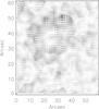 |
Fig. 1 Horizontal velocity at time 12 h, spatial and temporal window 3′′ and 30 min. The supergranule field is centered on (24′′, 39′′). |
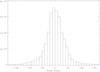 |
Fig. 2 Histogram of horizontal velocity directions deduced from the LCT (solid line). A Gaussian fit (dotted line) is superimposed. |
4. Link between exploding granules and large amplitude divergence
An important point to elucidate is the origin of large-scale positive divergences in the TFG and their link with horizontal velocity flow.
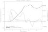 |
Fig. 3 Area of the largest TFG (number 129771, solid line), mean velocity divergence (dashed line) and expansion velocity (dotted line). |
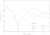 |
Fig. 4 Highest horizontal velocity of the five largest TFGs in the supergranule. |
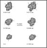 |
Fig. 5 Evolution of a new family of granules (TFG No. 129771) where exploding granules are indicated by arrows. The dark bar gives the scale of 5′′. |
Figure 3 shows family of the supergranule (number 129771) that is the strongest in space and time. It develops from time t = 3 h of the sequence and covers the greatest extent of the solar surface at t = 13 h after which it remains approximately stationary. The average value of the velocity divergence is always positive and highest at the beginning of the family development. The expansion velocity (defined as the time derivative of the square root of the family surface) is also highest (0.9 km s-1) at the beginning, meanwhile the maximum horizontal velocity also attains 0.9 km s-1. It is important to note that high divergences and velocities continue to be observed after the family has developed. This means that granules explode permanently in the family.
In Fig 4, the highest horizontal velocity is measured in the five strongest families of the supergranule. The largest family is No. 129771 and reaches 1.0 km s-1. Families often compete when they develope together. Maxima appear at times t = 1.5, 5, 12, 14 and 17 h where each maximum contributes to the migration of magnetic elements toward the boundaries. Their maxima are not in phase but in sequence, allowing a collective action in time to spread the magnetic field across the solar surface toward the network.
4.1. Birth and evolution of TFG
The TFG evolution shows successive explosions of granules at the beginning. At this stage, these explosions appear quasi-simultaneous. Figure 5 displays a family evolution at each step of a new generation of the tree (the time origin is the time of the first granule explosion of the TFG); arrows indicate the location of the observed explosions. From one generation to the next, the number of exploders may increase. The quasi-simultaneity of explosions is remarkable until up to five successive generations; then explosions shift from one generation to the next as a result of small cumulative phase shifts observed from the beginning. Figure 6 shows a temporal slice of a TFG (the same as in Fig. 5) where the V shape indicates the location of exploding granules. This shows the link between numerous exploding granules and the development of the TFG in the first three hours.
The time difference between two successive explosions is generally in the range of 8 to 10 min, then the granule children explode more or less in phase at the same time. This quasi-simultaneity of explosions at the beginning of a new TFG produces collective effects on the TFG expansion but also on the horizontal velocity fields. In particular, we observe (Fig. 3) a broad divergence of the flow at the location of the new TFG which later decreases. The largest area in Fig. 3 (around 13:00 and 16:00) is related to an increase of 73% of exploding granules in the TFG relative to the minimum at 14:30.
During its lifetime, the TFG shows variations related to new coherent exploding granules in the tree, which create new branches.
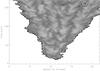 |
Fig. 6 V-shape temporal slice of successive exploding granules of a TFG (No. 129771). |
4.2. Relation of divergence and horizontal velocity
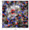 |
Fig. 7 Evolution of the properties of a supergranular cell. An animation is available online. See the appendix for details. Horizontal velocity amplitude (grayscale) in the sub-FoV. The divergence field is represented in red (positive) and blue (negative). The LoS magnetic field contour is shown in yellow and white (positive and negative polarities). |
The divergence field (length scale between 2 and 7 arcsec) is shown in Fig. 7 together with horizontal velocities Vh_mag and longitudinal magnetic fields at time 05:36 of the sequence. The strongest Vh_mag are located on the edge of divergences showing a clear link between them and horizontal flows inside the supergranule. The divergence in the central part of the FOV issued from a new TFG (23′′, 34′′) exhibits high Vh_mag in its lower part, although in its upper part (10′′, 48′′) only low Vh_mag is observed. This asymmetry is due to the presence of another divergence produced by a neighboring TFG (28′′, 40′′). Horizontal flows in between are opposite in direction, resulting in weak velocity flow that is due to mutual interaction. In contrast, TFG interactions may add to generate large-scale Vh_mag (few arcsec) which are important to drag the magnetic elements across the solar surface.
Panel 6 of Fig. 7 shows the temporal evolution of Vh_mag, divergences, and magnetic fields during 24 h in the same FOV as panel 1. First we note that NE magnetic fields are located in the converging flows that delineate the supergranule. This movie shows the links between positive divergences and Vh_mag. Strong Vh_mag occur where no opposite flow is created by other divergences in the vicinity. Successive divergences may have a cumulative effect on the final Vh_mag amplitude. Then the space and time coherence of the divergence appears crucial for the magnitude on the horizontal flow. Collective effects reinforce the Vh_mag field. Observed Vh_mag are in phase on scales of several arcsec and propagate velocity fronts across the solar surface.
In panel 7 the strongest divergences are located in the family; at the TFG birth, positive divergence is observed and the highest divergence magnitude corresponds to new branches of the TFG that grow quickly.
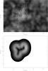 |
Fig. 8 Horizontal velocity amplitude field (gray levels) overlapped by intensity contour of the observed five exploding granules (top). Horizontal velocity amplitude (gray levels) of the five simulated exploding granules (bottom). |
Panel 8 shows the relation between the strongest positive divergence, Vh_mag, and the families. It allows us to describe the evolution of the family and divergences. At the emergence of a new family, a new positive divergence arises and generates strong horizontal flows which then propagate across the surface. During their travel, new flows combine with preexisting flows and thus generate the observed Vh_mag, which is modulated by collective effects.
4.3. Model of the collective effect of exploding granules
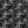 |
Fig. 9 Evolution of the exploding granules (contours) and amplitude of horizontal velocities (gray levels). The white bar gives a scale of 5′′. |
To model the collective effect of exploding granules on the flow, we simulated exploding granules by the function V(r) = Vexp × (r/R) × exp(−(r/R)2), where Vexp is the amplitude velocity, R the radius of the granule and r the distance from the granule center. Figure 8 shows the comparison of horizontal velocity magnitudes issued from the simultaneous explosion of five granules and compare them with those observed at t = 3112 s on the Sun. In this simulation the parameters are Vexp = 1.33 km s-1 and R = 3000 km. The simulation forms the highest velocity at the edge of the group of five exploding granules. The simultaneous explosions produce a collective effect on the flow with length greater than the size of granules up to several arcsec. Figure 9 shows the temporal evolution of the outlined intensity of the granules superimposed on the horizontal velocities Vh_mag. This confirms that larger amplitudes of velocities are at the edge of the family where explosions are strongest. However, departures between observed and simulated highest velocities might also be explained by the difference in the expansion rate of the solar explosive granules (which was chosen to be uniform in the simulation) or by the small phase shift between explosions of granules, which are neglected in the model.
5. Dynamical properties of the TFG and relation with horizontal velocity magnitude
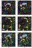 |
Fig. 10 Evolution of the properties of a supergranular cell. An animation is available online. See Appendix A for details. Top left: horizontal velocity magnitude Vh_mag (gray levels) and families (TFG) at time 05:02. Top right: same plot at 05:36; families are represented by various individual colors. Middle left: longitudinal magnetic field (yellow and white) and families (TFG) at time 05:02. Middle right: same plot at 05:36. Bottom left: horizontal velocity magnitude Vh_mag (gray levels), families (TFG), absolute value of the longitudinal magnetic field (white isocontours) and velocity divergence (blue for negative, yellow for positive) at time 05:02; bottom right: same plot at 05:36. |
The main goal of the present section is to determine how and where the velocity maxima Vh_mag are produced. Little is known about the dynamics on the intermediate timescales between one to several hours. Our preceding analysis Roudier et al. (2003) indicated that solar surface is structured by families of granules (TFG) that originate from a granule genitor. We observed that most of the granules on the solar surface belong to long-lived TFG. Each TFG is characterized by properties such as lifetime, size and expansion rate. The final area covered by the TFG seems to increase as a function of lifetime (Fig. 7 in Roudier et al. 2003).The largest TFGs are close in size to the smallest supergranules and we found that exploding granules play a major role in TFG evolution. In particular, we demonstrated that increases of the total area of families is related to granule explosions. A TFG can be viewed schematically as a series of branches corresponding to new generations of granules.
The evolution of horizontal velocities over a large FOV during 24 h reveals the locations of maxima of Vh_mag that coincide with the edges of the nascent TFG (see panel 9).
In panel 10 we observe the birth of different families; their expansion is associated with maxima of Vh_mag at the edge of TFGs and the motions of these maxima look like a wave propagating outward. Figure 10 (top) shows an example of such an evolution. In the central part of the figure a new TFG (green) forms around 05:02 and then expands; at 05:36, 32 min later, a maximum of horizontal velocity Vh_mag appears at the bottom edge of the TFG.
Panel 10 shows that the propagation of maxima is affected first by the growth of the family that initiated these maxima but also by the influence of other families. In some regions, Vh_mag maxima from different TFG may combine to form larger scale Vh_mag structures (see Panel 5).
Figure 10 (middle) shows that longitudinal magnetic fields are located at the edge of the TFG (both NE and IN). Vh_mag, families and the magnetic fields are shown together in Fig. 10 (bottom) and panel 8; we can follow the evolution of the large TFG (brown, in the center of the field) and Vh_mag maxima close to its borders. At 05:02, the new green TFG competes with the brown TFG . The maxima of Vh_mag around these two families are clearly visible at 05:40 of the 24-h sequence. The expansion speed of these two TFG vanishes along their common frontiers and causes an almost circular Vh_mag shape around the brown TFG on a scale between 10 to 15 arcsec. This is a good example of Vh_mag maxima generation by the evolving combination of strong adjacent TFG.
The entire sequence shows that the evolution of Vh_mag maxima is intimately related to the life of TFG through their location, strength, and birth date. Panels suggest a constant production rate of Vh_mag structures, with magnitudes related to the competing TFG in the FOV, but also to existing Vh_mag areas that are due to previous TFG that decline or have just disappeared. The frequent occurrence of Vh_mag patches and the interaction between families produces several events that contribute to the diffusion of the magnetic field and the photospheric network in the quiet Sun.
6. Intranetwork (IN) magnetic elements and cork evolution
6.1. Intranetwork magnetic elements
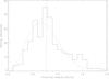 |
Fig. 11 Histogram of horizontal velocities for observed magnetic elements inside the supergranule (solid line). A Maxwellian fit (dotted line) is superimposed. |
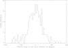 |
Fig. 12 Histogram of the angular distribution of the velocity vector of the IN magnetic elements with respect to the radial direction. |
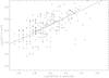 |
Fig. 13 Distance of magnetic elements to their starting point as a function of time (log log plot). |
The magnetic field in the quiet Sun is generally described as network (NE) and intranetwork (IN) components. The first represents the magnetic field that outlines the supergranulation boundaries, the second corresponds to small mixed-polarity elements inside the network. During the past decade numerous works have characterized the properties and dynamics of both IN and NE Gošić et al. (2014). The magnetic field emerges as ephemeral regions and weak-flux elements inside the IN; observations here reveal migrations of small sized-elements to supergranular boundaries.
In this section we focus on magnetic elements detected in Stokes V images during 24 h in the supergranule field. The magnetic network delineates a large supergranule that evolves continuously. The exposure time was rather short, therefore the signal-to-noise ratio of the V signal is limited and it was not possible to track many IN magnetic elements. An approximate value of the magnetic field, proportional to V/I, was derived using the usual weak-field approximation (panel 1).
Several magnetic elements (285 in total) were followed. We studied the statistics of their lifetimes. The median of the histogram was found at 800 s, but some elements lasted up to half an hour. When we eliminated ephemeral elements, the data were well fit by an exponential law of 500 s characteristic time. Figure 11 displays the velocity statistics. The median of the histogram is 0.8 km s-1. Velocities are more or less properly fitted by a Maxwellian law. Figure 12 shows the angular distribution of the velocity vector of the IN magnetic elements with respect to the radial direction (from the supergranule center at (24′′, 39′′), showing that outward motions dominate. Most of the velocity vectors of the IN magnetic elements (70%) are measured between ± 45°; this result fully corroborates those obtained from the LCT (Fig. 2).
Hagenaar et al. (1999) found evidence that in addition to the random walk corresponding to granulation, motions of magnetic elements are dominated by supergranulation on longer time scale. In panel 1 (magnetic field evolution) we observe both motions (random and radial) of the IN magnetic elements, but the small number of elements (due to the low sensitivity in Stokes V/I of our data) does not allow us to achieve a good statistical analysis of the random motions. Nevertheless, panel 2 clearly shows the random motions of the IN elements when they are located inside a TFG, and the systematic shift (toward the borders of the supergranule) is observed when they are located at the edge of a TFG. This agrees with the results obtained by Orozco Suárez et al. (2012b). The IN elements are continuously advected by large-scale convective flows, although on short timescales the velocity is dominated by granular motions or other effects. The highest horizontal velocities, generated by the TFG, might be the component that transports magnetic elements on long timescales. These velocities exhibit a spatial coherence at long times and large spatial scales that favor magnetic field diffusion on similar scales. The motion of the most important TFG in the supergranule shows that five of them are enough to build the network in six hours and then deform it the six following hours (see below).
The transport of the magnetic element in the photosphere is well described by a power law ⟨ (Δr)2 ⟩ = ctγ where ⟨ (Δr)2 ⟩ is the mean square displacement, c a constant, t is the time measured since the first detection, and γ is the spectral index Giannattasio et al. (2014b). The distance of magnetic elements to their starting point is plotted in Fig. 13 as a function of time. The slope of the linear fit (γ = 1.57) corresponds to a super-diffusive regime and agrees with previous results by Giannattasio et al. (2014b,a) and Del Moro et al. (2015). This suggests that advection might be the dominant mechanism related to large spatial and long timescales because TFG expansion produces the horizontal flow field.
6.2. Cork evolution
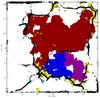 |
Fig. 14 Cork locations (white cross) at the end of the 24-h sequence in the supergranule field; the corks are swept out at the border of the supergranule where the magnetic field is anchored. The most important families (three) at the end of the sequence are overplotted in various colors. |
The evolution of an initially randomly distributed passive scalar (corks) is the best way to characterize the transport properties of the turbulent velocity field of the solar surface. Thousands of corks randomly distributed at initial time t = 0 and their surface distribution is followed during the whole sequence as they are advected by the horizontal velocity field. Figure 14 displays the cork distribution that results from the TFG evolution. This figure shows that a few families (three), which represent 80% of the total area, are enough to disseminate the corks to the edge of the supergranule. The largest families contribute to the evacuation of corks to the places where the magnetic network is located. The combined action of two (or more) large families that form close in time and space pushes corks out on tens of arcsec scales (mesoscale). This suggests that the distribution of the magnetic field on the solar surface depends on the most energetic TFG to form the photospheric network or magnetic patches. Small families, which are the most numerous, seem to play a minor role in the network building.
Figure 15 shows the cork trajectories (a selection of them for readability) during the full sequence relative to the magnetic network. The corks move almost radially toward the places of the magnetic network.
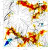 |
Fig. 15 Cork trajectories during the 24-h sequence in the supergranule field; only a few of them are plotted for clarity. Longitudinal magnetic fields of the network located around the supergranule are overplotted in blue and red colors. |
Panel 3 shows the full evolution of corks relative to the families. We observe the rapid expulsion of corks from the TFG and the advection of corks toward supergranule boundaries. In addition, panel 4 shows that during their journey corks are mainly located inside the supergranule where the IN magnetic field is. Both movies indicate the close link between TFG and magnetic element evolution inside the supergranule.
7. Link between horizontal velocities and magnetic elements
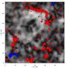 |
Fig. 16 Evolution of the properties of a supergranular cell. An animation is available online. See the appendix for details. Horizontal velocity Vh_mag (gray levels) at time 422.5 min of the sequence. The longitudinal magnetic field is overplotted (blue and red). |
The IN flux is found to be the most important contributor to the NE and was able to replace its entire flux in 18 to 24 h Gošić et al. (2014). According to these authors the small-scale IN elements appear as the most permanent source of flux for the NE. The maintenance of the NE requires the transport of the IN elements across the solar surface toward the edges of supergranules; this process is not well documented as yet.
To obtain more details of the magnetic element transport in the quiet Sun, we reexamined the 2007 Hinode data Roudier et al. (2009) with particular attention to the amplitude of the horizontal velocity field. Figure 16 (and panel 5) shows the horizontal velocity magnitude (Vh_mag) and the longitudinal magnetic field during 24 h, in the closed-network region (supergranule field).
The locations where the Vh_mag has the largest amplitude appear to play an overriding role in the network formation and evolution (deformation and localization). The movie (panel 5) reveals that the motions of the magnetic elements inside the supergranule are driven by Vh_mag flows regardless of their locations. In the IN, the magnetic field elements (regardless of their polarity) are clearly swept out (advected or diffused) toward the supergranule borders by Vh_mag horizontal flow fronts across several arcsec with amplitudes between 0.5 and 0.8 km s-1.
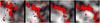 |
Fig. 17 Temporal evolution of Vh_mag (gray levels) and longitudinal magnetic field (blue and red) around coordinates (40′′, 52′′) (upper left corner of the supergranule field). From left to right times are 59 min, 169 min, 261 min and 377 min; the FOV is 18.6″ × 18.1″. The white bar gives a scale of 5′′. |
As previously described by Roudier et al. (2009), the geometric evolution of the network is linked to the TFG expansion (more details below). Here, we observe a clear evolution of the network shape and location also driven by Vh_mag (Fig. 17). We note that magnetic network patches are pushed when there are no (or lower) horizontal velocities on the opposite side of the patch. If similar amplitudes of Vh_mag are observed (right part of Fig. 17, time = 377 min) on both sides of the NE, the patch remains stable (see also another example in the bottom left part of the field in the middle of panel 5). The shape of the network and the flux inflow from IN to NE is strongly linked to the Vh_mag evolution. The strongest and largest occurrences of Vh_mag appear to be one of the most important component occurrences to structure the network. The temporal coherence of Vh_mag between one to two hours andon a spatial scale between 3′′ to 12′′ also seems to play a major role. In the central part of the movie (panel 5), the supergranule is clearly outlined by magnetic fields although in other parts (left upper side in Fig. 16) the network contour is less visible because of the lower horizontal velocities. This property may be able to explain why the network appears more or less closed at supergranular scale.
During the 24 h, the supergranule delineated by the longitudinal magnetic field appears to move toward the right side of the FOV. This is quite surprising because a detailed check of our data alignment did not show any drift, whereas the NE appears to rotate 6% faster. We observe, as Langfellner et al. (2015), a greater presence of the NE in the western part (Fig. 16) of the supergranule.
8. Discussion
The origin and detailed evolution of the supergranulation is still an open question. The supergranular flow scale is unexplained. The length scale (30 Mm) and lifetime (24 to 48 h) promote studies with low resolutions DeRosa & Toomre (2004). Statistical averaging over measurements of numerous supergranules (DeGrave & Jackiewicz 2015; Duvall et al. 2014; Langfellner et al. 2015) allows us to describe global characteristics, but it is difficult to identify the mechanism of supergranule formation because a correspondence between average quantities and the high temporal and spatial processes is missing.
Supergranules are often described as convective structures with an upflowing central region, horizontally diverging flows, and downflows at the edge. Because downflows are co-spatial with magnetic elements, many authors have argued that supergranulation is a magnetoconvection phenomenon Berrilli et al. (1999). However, simulations do not agree on the causal mechanism and helium ionization is invoked Hanasoge & Sreenivasan (2014).
Supergranulation is often described as an isotropic flow diffusing magnetic fields toward their periphery. From an observational point of view, the large-scale structure is inhomogeneous in size, velocity magnitude and shape (see Fig. 3 of Rieutord & Rincon 2010 issued from the largest high-resolution FOV of horizontal velocities up to now). This reveals the anisotropic character of flows, which has consequences on the diffusion of magnetic fields across the solar surface on a long timescale. The NE outlines supergranular cells Rutten (1999) but is often incomplete at the boundaries. The magnetic NE is quite fragmented and exhibits many patches of strong fields coinciding with vertices where supergranular flows meet, presumably marking the sites of downflows required by mass conservation Hagenaar et al. (1999). This also raises the question of the link between flows and NE formation. In addition, recent works using helioseismic data emphasized the difficulty of deriving the formation height of the supergranulation, as well as the velocity profile with altitude DeGrave & Jackiewicz (2015). This means that the supergranular model with warmer fluid upflowing at the center and cooler fluid downflowing at the boundaries is not supported by observations (see also Rast 2003).
The high spatial and temporal resolution of Hinode/SOT data allowed us to study great detail the evolution of the photospheric flows relative to TFG that cover the solar surface for 24 h . Large TFGs, with sizes close to supergranulation, are not numerous but are sufficient to structure the flows. TFGs grow in area by a succession of granule explosions that are correlated in time. TFGs and their mutual interactions are able to sweep out magnetic elements to the border of supergranules. Almost simultaneous explosions of granules at TFG birth generate coherent flow fronts with large spatial scales (3 to 12′′) and long lifetimes (one to two hours) with magnitudes in the range 0.5 to 0.8 km s-1. New branches of TFGs during their life generate collective effects through horizontal velocities that supply the general flow. Flow fronts propagate when there is no counterpart motion resulting from interactions with other TFG. Horizontal flows tend to increase close to the limits of expanding TFGs, extracting out magnetic elements more or less radially toward the borders of supergranules. The occurrence of large-scale velocity maxima is probably one of the main phenomena that diffuse (or advect) the magnetic field and also affect the NE shape and evolution. Magnetic patches in the IN are found at the edge of velocity fronts, indicating a possible link between IN and TFG evolution. The lack of the magnetic signal observed at the center of supergranules Stangalini (2014) might be related to the formation and evolution of TFGs that quickly expels corks that are considered to be proxies of magnetic flux tubes.
The velocity fronts produced by the TFG may not only contribute to magnetic diffusion in supergranules but also be generated by small-scale dynamo Tobias & Cattaneo (2008). Tobias and Cattaneo showed that the magnetic field amplification depends on spatially and temporally coherent structures.
We observed an intriguing event in the evolution of the NE: while data alignment was perfectly controlled during 24 h (solar rotation and satellite shifts where corrected for), the NE moved to the right side of the FOV (6% faster westward). This is quite difficult to interpret in the context of the classical convective approach of the supergranulation. Motions of NE patches appear to be governed by the largest TFG expansion and the resulting horizontal flows. We suggest that NE location and shape are controlled by TFG evolution in space and time. The new question arising from our analysis is whether TFGs are only the basic elements of supergranules or the main structure at the origin of NE formation and evolution. We cannot answer this question; numerical simulations could help to distinguish between these hypotheses, however.
9. Conclusions
Understanding the mechanism that diffuses magnetic fields is still a challenge. This important, because the NE contribution to the global solar magnetism is known to be similar to the flux of active regions at maximum activity.
From our analysis at high spatial and temporal resolution during 24 h, TFGs appear as one of the main elements of supergranules which diffuse and advect magnetic fields over the solar surface. We discovered that the largest TFG evolutions and mutual interactions produce cumulative effects that are able to build horizontally coherent flows with longer lifetimes than granulation (one to two hours) and with scale lengths of up to 12′′. We observed that TFGs grow in area by a succession of granule explosions, which are correlated in time, expelling corks on the typical size of the mesoscale. Diverging flows at the beginning of TFG life generate horizontal and outward velocity fronts with magnitudes between 0.5 and 0.8 km s-1 over several arcsec.
These coherent flows are often located at TFG edges and can propagate in the direction where they do not need to compete with another large TFG. The flows act on the location and shape of the NE and are compatible with the recent work of Gošić et al. 2014 who indicated that the IN might supply the magnetic flux in the NE in only 9 to 13 h. We suggest that supergranular NE might be a spatial pattern that originates from the action of TFGs on the scale of supergranules.
The rotation of the NE (6% faster westward) found in our data raises the question of the role of TFGs on the solar surface. TFG flows might be the origin of NE formation by feeding and shaping it. We must now test this conjecture by analyzing simulations with large FOVs with known parameters to determine whether TFGs are able to provide sufficient diffusion rates to
account for large-scale distribution of the magnetic fields in the solar photosphere Simon et al. (1995).
Online material
Movie of Fig. A.1 Access Supplementary Material
Movie of Fig. A.1 Access Supplementary Material
Acknowledgments
We thank the Hinode/SOT team for assistance in acquiring and processing the data. Hinode is a Japanese mission developed and launched by ISAS/JAXA, collaborating with NAOJ as a domestic partner, NASA and STFC (UK) as international partners. Support for the post-launch operation is provided by JAXA and NAOJ (Japan), STFC (UK), NASA, ESA, and NSC (Norway). This work was granted access to the HPC resources of CALMIP under the allocation 2011-[P1115]. The authors wish to thank the anonymous referee for very helpful comments and suggestions that improved the quality of the manuscript.
References
- Berrilli, F., Ermolli, I., Florio, A., & Pietropaolo, E. 1999, A&A, 344, 965 [NASA ADS] [Google Scholar]
- Crouch, A. D., Charbonneau, P., & Thibault, K. 2007, ApJ, 662, 715 [NASA ADS] [CrossRef] [Google Scholar]
- DeGrave, K., & Jackiewicz, J. 2015, Sol. Phys., 290, 1547 [NASA ADS] [CrossRef] [Google Scholar]
- Del Moro, D., Giannattasio, F., Berrilli, F., et al. 2015, A&A, 576, A47 [NASA ADS] [CrossRef] [EDP Sciences] [Google Scholar]
- DeRosa, M. L., & Toomre, J. 2004, ApJ, 616, 1242 [NASA ADS] [CrossRef] [Google Scholar]
- Duvall, T. L., Hanasoge, S. M., & Chakraborty, S. 2014, Sol. Phys., 289, 3421 [NASA ADS] [CrossRef] [Google Scholar]
- Giannattasio, F., Berrilli, F., Biferale, L., et al. 2014a, A&A, 569, A121 [NASA ADS] [CrossRef] [EDP Sciences] [Google Scholar]
- Giannattasio, F., Stangalini, M., Berrilli, F., Del Moro, D., & Bellot Rubio, L. 2014b, ApJ, 788, 137 [NASA ADS] [CrossRef] [Google Scholar]
- Gošić, M., Bellot Rubio, L. R., Orozco Suárez, D., Katsukawa, Y., & del Toro Iniesta, J. C. 2014, ApJ, 797, 49 [NASA ADS] [CrossRef] [Google Scholar]
- Hagenaar, H. J., Schrijver, C. J., Title, A. M., & Shine, R. A. 1999, ApJ, 511, 932 [NASA ADS] [CrossRef] [Google Scholar]
- Hanasoge, S. M., & Sreenivasan, K. R. 2014, Sol. Phys., 289, 3403 [NASA ADS] [CrossRef] [Google Scholar]
- Hart, A. B. 1954, MNRAS, 114, 17 [NASA ADS] [CrossRef] [Google Scholar]
- Langfellner, J., Gizon, L., & Birch, A. C. 2015, A&A, 579, L7 [NASA ADS] [CrossRef] [EDP Sciences] [Google Scholar]
- Leighton, R. B., Noyes, R. W., & Simon, G. W. 1962, ApJ, 135, 474 [NASA ADS] [CrossRef] [Google Scholar]
- November, L. J. 1989, ApJ, 344, 494 [NASA ADS] [CrossRef] [Google Scholar]
- Orozco Suárez, D., Bellot Rubio, L. R., & Katsukawa, Y. 2012a, in Second ATST-EAST Meeting: Magnetic Fields from the Photosphere to the Corona, eds. T. R. Rimmele, A. Tritschler, F. Wöger, et al., ASP Conf. Ser., 463, 57 [Google Scholar]
- Orozco Suárez, D., Katsukawa, Y., & Bellot Rubio, L. R. 2012b, ApJ, 758, L38 [NASA ADS] [CrossRef] [Google Scholar]
- Rast, M. P. 2003, ApJ, 597, 1200 [NASA ADS] [CrossRef] [Google Scholar]
- Rieutord, M., & Rincon, F. 2010, Liv. Rev. Sol. Phys., 7, 2 [Google Scholar]
- Roudier, T., Rieutord, M., Malherbe, J., & Vigneau, J. 1999, A&A, 349, 301 [NASA ADS] [Google Scholar]
- Roudier, T., Lignières, F., Rieutord, M., Brandt, P. N., & Malherbe, J. M. 2003, A&A, 409, 299 [NASA ADS] [CrossRef] [EDP Sciences] [Google Scholar]
- Roudier, T., Rieutord, M., Brito, D., et al. 2009, A&A, 495, 945 [NASA ADS] [CrossRef] [EDP Sciences] [Google Scholar]
- Rutten, R. J. 1999, in Third Advances in Solar Physics Euroconference: Magnetic Fields and Oscillations, eds. B. Schmieder, A. Hofmann, & J. Staude, ASP Conf. Ser., 184, 181 [Google Scholar]
- Simon, G. W., Title, A. M., & Weiss, N. O. 1995, ApJ, 442, 886 [NASA ADS] [CrossRef] [Google Scholar]
- Stangalini, M. 2014, A&A, 561, L6 [NASA ADS] [CrossRef] [EDP Sciences] [Google Scholar]
- Stein, R. F., Nordlund, Å., Georgoviani, D., Benson, D., & Schaffenberger, W. 2009, in Solar-Stellar Dynamos as Revealed by Helio- and Asteroseismology: GONG 2008/SOHO 21, eds. M. Dikpati, T. Arentoft, I. González Hernández, C. Lindsey, & F. Hill, ASP Conf. Ser., 416, 421 [Google Scholar]
- Suematsu, Y., Tsuneta, S., Ichimoto, K., et al. 2008, Sol. Phys., 249, 197 [NASA ADS] [CrossRef] [Google Scholar]
- Tobias, S. M., & Cattaneo, F. 2008, Phys. Rev. Lett., 101, 125003 [NASA ADS] [CrossRef] [Google Scholar]
Appendix A: Evolution of a supergranule
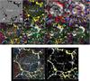 |
Fig. A.1 Evolution of the magnetic field and several derived properties as discussed in the main text (snapshot of the movie). The field of view (60″ × 62″) and is centered on the well-formed superganule with an almost closed magnetic network at the boundaries. The time step is 50 s between each frame and the duration is 24 h (1716 frames). The pixel size is 0.16′′. The contents of the individual panels is as follows: Panel 1) evolution of the magnetic field . Panel 2) evolution of the TFG with various colors; the longitudinal magnetic field is superimposed (yellow and white). Panel 3) evolution of corks (indicated by crosses) relative to the TFG (various colors); the longitudinal magnetic field is superimposed (yellow and blue). Panel 4) evolution of corks (indicated by crosses) relative to the intranework (IN) and network (NE) longitudinal magnetic field (yellow and blue). Panel 5) evolution of horizontal velocity magnitudes (Vh_mag, gray levels) and the longitudinal magnetic field (red and blue). Panel 6) evolution of horizontal velocity magnitudes Vh_mag, divergence of horizontal velocities (positive for divergent in red, negative for convergent in blue) together with magnetic fields (yellow and white contours). Panel 7) evolution of the positive divergence (in red) relative to the families (TFG in various colors) and magnetic fields (yellow and blue). Panel 8) evolution of the positive divergence (in blue) relative to the families (TFG in various colors), magnetic field magnitude (white contours) and horizontal velocity magnitudes Vh_mag (gray levels). Panel 9) evolution of the families (TFG in various colors), horizontal velocity magnitudes Vh_mag (white) and magnetic fields (yellow and blue contours). Panel 10) evolution of the families (TFG in various colors) and horizontal velocity magnitudes Vh_mag (white). The movies can be found in full resolution online or at: http://www.lesia.obspm.fr/perso/jean-marie-malherbe/Hinode2007/hinode2007.html. |
All Figures
|
Fig. 1 Horizontal velocity at time 12 h, spatial and temporal window 3′′ and 30 min. The supergranule field is centered on (24′′, 39′′). |
| In the text | |
|
Fig. 2 Histogram of horizontal velocity directions deduced from the LCT (solid line). A Gaussian fit (dotted line) is superimposed. |
| In the text | |
|
Fig. 3 Area of the largest TFG (number 129771, solid line), mean velocity divergence (dashed line) and expansion velocity (dotted line). |
| In the text | |
|
Fig. 4 Highest horizontal velocity of the five largest TFGs in the supergranule. |
| In the text | |
|
Fig. 5 Evolution of a new family of granules (TFG No. 129771) where exploding granules are indicated by arrows. The dark bar gives the scale of 5′′. |
| In the text | |
|
Fig. 6 V-shape temporal slice of successive exploding granules of a TFG (No. 129771). |
| In the text | |
|
Fig. 7 Evolution of the properties of a supergranular cell. An animation is available online. See the appendix for details. Horizontal velocity amplitude (grayscale) in the sub-FoV. The divergence field is represented in red (positive) and blue (negative). The LoS magnetic field contour is shown in yellow and white (positive and negative polarities). |
| In the text | |
|
Fig. 8 Horizontal velocity amplitude field (gray levels) overlapped by intensity contour of the observed five exploding granules (top). Horizontal velocity amplitude (gray levels) of the five simulated exploding granules (bottom). |
| In the text | |
|
Fig. 9 Evolution of the exploding granules (contours) and amplitude of horizontal velocities (gray levels). The white bar gives a scale of 5′′. |
| In the text | |
|
Fig. 10 Evolution of the properties of a supergranular cell. An animation is available online. See Appendix A for details. Top left: horizontal velocity magnitude Vh_mag (gray levels) and families (TFG) at time 05:02. Top right: same plot at 05:36; families are represented by various individual colors. Middle left: longitudinal magnetic field (yellow and white) and families (TFG) at time 05:02. Middle right: same plot at 05:36. Bottom left: horizontal velocity magnitude Vh_mag (gray levels), families (TFG), absolute value of the longitudinal magnetic field (white isocontours) and velocity divergence (blue for negative, yellow for positive) at time 05:02; bottom right: same plot at 05:36. |
| In the text | |
|
Fig. 11 Histogram of horizontal velocities for observed magnetic elements inside the supergranule (solid line). A Maxwellian fit (dotted line) is superimposed. |
| In the text | |
|
Fig. 12 Histogram of the angular distribution of the velocity vector of the IN magnetic elements with respect to the radial direction. |
| In the text | |
|
Fig. 13 Distance of magnetic elements to their starting point as a function of time (log log plot). |
| In the text | |
|
Fig. 14 Cork locations (white cross) at the end of the 24-h sequence in the supergranule field; the corks are swept out at the border of the supergranule where the magnetic field is anchored. The most important families (three) at the end of the sequence are overplotted in various colors. |
| In the text | |
|
Fig. 15 Cork trajectories during the 24-h sequence in the supergranule field; only a few of them are plotted for clarity. Longitudinal magnetic fields of the network located around the supergranule are overplotted in blue and red colors. |
| In the text | |
|
Fig. 16 Evolution of the properties of a supergranular cell. An animation is available online. See the appendix for details. Horizontal velocity Vh_mag (gray levels) at time 422.5 min of the sequence. The longitudinal magnetic field is overplotted (blue and red). |
| In the text | |
|
Fig. 17 Temporal evolution of Vh_mag (gray levels) and longitudinal magnetic field (blue and red) around coordinates (40′′, 52′′) (upper left corner of the supergranule field). From left to right times are 59 min, 169 min, 261 min and 377 min; the FOV is 18.6″ × 18.1″. The white bar gives a scale of 5′′. |
| In the text | |
|
Fig. A.1 Evolution of the magnetic field and several derived properties as discussed in the main text (snapshot of the movie). The field of view (60″ × 62″) and is centered on the well-formed superganule with an almost closed magnetic network at the boundaries. The time step is 50 s between each frame and the duration is 24 h (1716 frames). The pixel size is 0.16′′. The contents of the individual panels is as follows: Panel 1) evolution of the magnetic field . Panel 2) evolution of the TFG with various colors; the longitudinal magnetic field is superimposed (yellow and white). Panel 3) evolution of corks (indicated by crosses) relative to the TFG (various colors); the longitudinal magnetic field is superimposed (yellow and blue). Panel 4) evolution of corks (indicated by crosses) relative to the intranework (IN) and network (NE) longitudinal magnetic field (yellow and blue). Panel 5) evolution of horizontal velocity magnitudes (Vh_mag, gray levels) and the longitudinal magnetic field (red and blue). Panel 6) evolution of horizontal velocity magnitudes Vh_mag, divergence of horizontal velocities (positive for divergent in red, negative for convergent in blue) together with magnetic fields (yellow and white contours). Panel 7) evolution of the positive divergence (in red) relative to the families (TFG in various colors) and magnetic fields (yellow and blue). Panel 8) evolution of the positive divergence (in blue) relative to the families (TFG in various colors), magnetic field magnitude (white contours) and horizontal velocity magnitudes Vh_mag (gray levels). Panel 9) evolution of the families (TFG in various colors), horizontal velocity magnitudes Vh_mag (white) and magnetic fields (yellow and blue contours). Panel 10) evolution of the families (TFG in various colors) and horizontal velocity magnitudes Vh_mag (white). The movies can be found in full resolution online or at: http://www.lesia.obspm.fr/perso/jean-marie-malherbe/Hinode2007/hinode2007.html. |
| In the text | |
Current usage metrics show cumulative count of Article Views (full-text article views including HTML views, PDF and ePub downloads, according to the available data) and Abstracts Views on Vision4Press platform.
Data correspond to usage on the plateform after 2015. The current usage metrics is available 48-96 hours after online publication and is updated daily on week days.
Initial download of the metrics may take a while.