| Issue |
A&A
Volume 590, June 2016
|
|
|---|---|---|
| Article Number | A24 | |
| Number of page(s) | 8 | |
| Section | Extragalactic astronomy | |
| DOI | https://doi.org/10.1051/0004-6361/201527256 | |
| Published online | 02 May 2016 | |
MAGIC observations of the February 2014 flare of 1ES 1011+496 and ensuing constraint of the EBL density
1
ETH Zurich, 8093
Zurich,
Switzerland
2
Università di Udine and INFN Trieste, 33100
Udine,
Italy
3
INAF National Institute for Astrophysics,
00136
Rome,
Italy
4
Università di Siena, and INFN Pisa, 53100
Siena,
Italy
5
Croatian MAGIC Consortium, Rudjer Boskovic Institute, University
of Rijeka, University of Split and University of Zagreb, Zagreb, Croatia
6
Saha Institute of Nuclear Physics, 1\AF Bidhannagar, Salt Lake, Sector-1,
700064
Kolkata,
India
7
Max-Planck-Institut für Physik, 80805
München,
Germany
8
Universidad Complutense, 28040
Madrid,
Spain
9
Inst. de Astrofísica de Canarias, 38200 La Laguna, Tenerife,
Spain; Universidad de La Laguna, Dpto. Astrofísica, 38206
La Laguna, Tenerife,
Spain
10
University of Łódź, 90236
Lodz,
Poland
11
Deutsches Elektronen-Synchrotron (DESY),
15738
Zeuthen,
Germany
12
IFAE, Campus UAB, 08193
Bellaterra,
Spain
13
Universität Würzburg, 97074
Würzburg,
Germany
14
Centro de Investigaciones Energéticas, Medioambientales y
Tecnológicas, 28040
Madrid,
Spain
15
Università di Padova and INFN, 35131
Padova,
Italy
16
Institute for Space Sciences (CSIC\IEEC),
08193
Barcelona,
Spain
17
Technische Universität Dortmund, 44221
Dortmund,
Germany
18
Unitat de Física de les Radiacions, Departament de Física, and
CERES-IEEC, Universitat Autònoma de Barcelona, 08193
Bellaterra,
Spain
19
Universitat de Barcelona, ICC, IEEC-UB,
08028
Barcelona,
Spain
20
Japanese MAGIC Consortium, ICRR, The University of Tokyo,
Department of Physics and Hakubi Center, Kyoto University, Tokai University, The
University of Tokushima, KEK, Japan
21
Finnish MAGIC Consortium, Tuorla Observatory, University of Turku
and Department of Physics, University of Oulu, 90014
Oulu,
Finland
22
Inst. for Nucl. Research and Nucl. Energy,
1784
Sofia,
Bulgaria
23
Università di Pisa and INFN Pisa, 56126
Pisa,
Italy
24
ICREA and Institute for Space Sciences (CSIC\IEEC),
08193
Barcelona,
Spain
25
Università dell’Insubria and INFN Milano Bicocca,
Como, 22100
Como,
Italy
26
now at Centro Brasileiro de Pesquisas Físicas (CBPF\MCTI), R. Dr.
Xavier Sigaud, 150 – Urca, Rio de
Janeiro
22290-180 – RJ, Brazil
27
now at: NASA Goddard Space Flight Center, Greenbelt, MD 20771, USA
and Department of Physics and Department of Astronomy, University of
Maryland, College
Park, MD
20742,
USA
28
Humboldt University of Berlin, Istitut für Physik Newtonstr. 15, 12489
Berlin,
Germany
29
now at: École polytechnique fédérale de Lausanne
(EPFL), 1015
Lausanne,
Switzerland
30
also at: INFN, 35131
Padova,
Italy
31
now at: Laboratoire AIM, Service d’Astrophysique, DSM\IRFU,
CEA\Saclay 91191
Gif-sur-Yvette Cedex,
France
32
now at: Finnish Centre for Astronomy with ESO
(FINCA), 20014
Turku,
Finland
33
also at: INAF-Trieste
34
also at: ISDC – Science Data Center for
Astrophysics, 1290
Versoix
( Geneva )
35
now at: Instituto de Física, Universidad Nacional Autónoma de
México, Apartado Postal
20-364, 01000
México D. F.,
Mexico
Received:
25
August
2015
Accepted:
16
February
2016
Abstract
Context. During February–March 2014, the MAGIC telescopes observed the high-frequency peaked BL Lac 1ES 1011+496 (z = 0.212) in flaring state at very-high energy (VHE, E> 100 GeV). The flux reached a level of more than ten times higher than any previously recorded flaring state of the source.
Aims. To describe the characteristics of the flare presenting the light curve and the spectral parameters of the night-wise spectra and the average spectrum of the whole period. From these data we aim to detect the imprint of the extragalactic background light (EBL) in the VHE spectrum of the source, to constrain its intensity in the optical band.
Methods. We analyzed the gamma-ray data from the MAGIC telescopes using the standard MAGIC software for the production of the light curve and the spectra. To constrain the EBL, we implement the method developed by the H.E.S.S. collaboration, in which the intrinsic energy spectrum of the source is modeled with a simple function (≤4 parameters), and the EBL-induced optical depth is calculated using a template EBL model. The likelihood of the observed spectrum is then maximized, including a normalization factor for the EBL opacity among the free parameters.
Results. The collected data allowed us to describe the night-wise flux changes and also to produce differential energy spectra for all nights in the observed period. The estimated intrinsic spectra of all the nights could be fitted by power-law functions. Evaluating the changes in the fit parameters, we conclude that the spectral shape for most of the nights were compatible, regardless of the flux level, which enabled us to produce an average spectrum from which the EBL imprint could be constrained. The likelihood ratio test shows that the model with an EBL density 1.07 (–0.20, +0.24)stat+sys, relative to the one in the tested EBL template, is preferred at the 4.6σ level to the no-EBL hypothesis, with the assumption that the intrinsic source spectrum can be modeled as a log-parabola. This would translate into a constraint of the EBL density in the wavelength range [0.24 μm, 4.25 μm], with a peak value at 1.4 μm of λFλ = 12.27-2.29+2.75 nW m-2 sr-1, including systematics.
Key words: BL Lacertae objects: general / intergalactic medium / cosmic background radiation
Corresponding authors: A. González Muñoz This email address is being protected from spambots. You need JavaScript enabled to view it. ; A. Moralejo This email address is being protected from spambots. You need JavaScript enabled to view it. ; and P. Bangale This email address is being protected from spambots. You need JavaScript enabled to view it.
© ESO, 2016
1. Introduction
1ES 1011+496 (RA: 10h15m04.1s, Dec: + 49°26m01s) is an active galactic nucleus (AGN) classified as a high-frequency peaked BL Lac (HBL), which is located at redshift = 0.212 (Albert et al. 2007). HBLs have spectral energy distributions (SED) that are characterized by two peaks, one located in the UV to soft X-ray band, and the second located in the GeV to TeV range, which makes it possible to detect them in very-high-energy (VHE, E> 100 GeV) γ rays. 1ES 1011+496 was discovered at VHE by the MAGIC Collaboration in 2007, following an optical high state reported by the Tuorla Blazar Monitoring Programme (Albert et al. 2007).
The observation of a bright source at intermediate redshift, like 1ES 1011+496, provides a good opportunity to constrain the impact of the extragalactic background light (EBL) on the propagation of γ rays over cosmological distances. The EBL is the diffuse radiation that comes from the contributions of all the light emitted by stars in the UV-optical and near infrared (NIR) bands. It also contains the infrared (IR) radiation emitted by dust after absorbing the starlight, plus a small contribution from AGNs (Hauser & Dwek 2001). VHE γ rays from extragalactic sources interact with the EBL in the optical and NIR bands, producing electron-positron pairs, which causes an attenuation of the VHE photon flux measured at Earth (Gould & Schréder 1967).
Measuring the EBL directly is a challenging task owing to the intense foreground light from interplanetary dust. Strict lower limits to the EBL have been derived from galaxy counts for the optical band (Madau & Pozzetti 2000; Fazio et al. 2004; Dole et al. 2006). At NIR wavelengths, one way to access the EBL is by large-scale anisotropy measurements (e.g. Cooray et al. 2004; Fernandez et al. 2010; Zemcov et al. 2014). Making reasonable assumptions on the intrinsic VHE spectra of extragalactic sources (e.g. the limit in the hardness of the photon spectra of 1.5, coming from theoretical limits in the acceleration mechanisms), upper limits to the EBL density can be derived (e.g. Stecker & de Jager 1996; Aharonian et al. 2006; Mazin & Raue 2007). More recently, extrapolations of data from the Fermi Large Area Telescope have been used to set constraints to the intrinsic VHE spectra of distant sources which, in combination with Imaging Atmospheric Cherenkov Telescopes (IACT) observations of the same objects, have also provided upper limits to the EBL density (Georganopoulos et al. 2010; Orr et al. 2011; Meyer et al. 2012).
The Fermi collaboration employed a different technique to constrain the EBL density using a likelihood ratio test on LAT data from a number of extragalactic sources (Ackermann et al. 2012). SEDs from 150 BL Lacs in the redshift range 0.03–1.6 were modeled as log parabolae in the optically-thin regime (E< 25 GeV), then extrapolated to higher energies and compared with the actually observed photon fluxes. A likelihood ratio test was used to determine the best-fit scaling factor for the optical depth τ(E,z) according to a given EBL model, hence providing constraints of the EBL density relative to the model prediction. Several EBL models were tested using this technique (e.g. Stecker et al. 2006; Finke et al. 2010), including the most widely and recently used by IACTs by Franceschini et al. (2008) and Domínguez et al. (2011). They obtained a measurement of the UV component of the EBL of 3 ± 1 nW m-2 sr-1 at z ≈ 1.
The H.E.S.S. collaboration used a similar likelihood ratio test to constrain the EBL, taking advantage of their observations of distant sources at VHE (Abramowski et al. 2013). The EBL absorption at VHE is expected to leave an imprint in the observed spectra, coming from a distinctive feature (an inflection point in the log flux-log E representation) between ~100 GeV and ~5–10 TeV, a region observable by IACTs. This feature is due to a peak in the optical region of the EBL flux density, which is powered mainly by starlight. The H.E.S.S. collaboration modeled the intrinsic spectra of several AGNs using simple functions (up to 4 parameters), then applied a flux suppression factor exp(−α × τ(E,z)), where τ is the optical depth according to a given EBL model and α, a scaling factor. A scan over α was performed to achieve the best fit to the observed VHE spectra. The no-EBL hypothesis, α = 0, was excluded at the 8.8σ level, and the EBL flux density was constrained in the wavelength range between 0.30 μm and 17 μm (optical to NIR) with a peak value of 15 ± 2stat ± 3sys nW m-2 sr-1 at 1.4 μm.
In Domínguez et al. (2013), data from 1ES 1011+496 was used as part of a data set from several AGNs to measure the cosmic γ-ray horizon (CGRH). The CGRH is defined as the energy at which the optical depth of the photon-photon pair production becomes unity as function of energy. Using multi-wavelenght (MWL) data, Domínguez et al. modeled the SED of each source, including 1ES 1011+496, doing a extrapolation to the VHE band. Then they made a comparison with the observed VHE data. In the case of 1ES 1011+496, they modeled the SED using the optical data from 2007 (Albert et al. 2007) and X-ray data (from the X-Ray Timing Explorer) taken in 2008 May, and compared it with the VHE data taken in 2007 by MAGIC. Their prediction was below the observed VHE data, which led to no optical-depth information. The prediction may have failed owing to the lack of simultaneity in the data. A similar approach was presented by Mankuzhiyil et al. (2010), where they modeled the SED of PKS 2155-304, making a prediction for the VHE band, and compared it to the observed data to give attenuation limits.
After the discovery of 1ES 1011+496 in 2007 (Albert et al. 2007), two more multi-wavelength campaigns were organised by MAGIC: the first one between March and May 2008 (Ahnen et al. 2016) and a second one divided in two periods, from March to April 2011 and from January to May 2012 (Aleksic et al. 2016). In all previous observations (including the discovery) the source did not show evidence of flux variability within the observed periods and the observed spectra could be fitted with simple power-law functions, with photon indices ranging from 3.2 ± 0.4stat to 4.0 ± 0.5stat, and integral fluxes, above 200 GeV, between (0.8 ± 0.1stat) × 10-10 and (1.6 ± 0.3stat) × 10-11 photons cm-2 s-1.
In this paper we present the analysis of the extraordinary flare of 1ES 1011+496 between February–March 2014 that was observed by the MAGIC telescopes, and apply a technique based on Abramowski et al. (2013) to constrain the EBL. The observations and the data reduction are described in Sect. 2, the results in Sect. 3, the procedure for constraining the EBL in Sect. 4, the inclusion of the systematic uncertainty is shown in Sect. 5, and the results of the EBL constraint are discussed in Sect. 6.
2. Observations and analysis
MAGIC is a stereoscopic system of two 17 m diameter Imaging Atmospheric Cherenkov Telescopes (IACT) situated at the Roque de los Muchachos, on the Canary island of La Palma (28.75°N, 17.86°W) at a height of 2200 m above sea level. Since the end of 2009, it has been working in stereoscopic mode with a trigger threshold of ~50 GeV. During 2011 and 2012, MAGIC underwent a series of upgrades which resulted in a sensitivity of (0.66 ± 0.03)% of the Crab nebula flux above 220 GeV in 50 h at low zenith angles (Aleksić et al. 2015a,b).
On February 5 2014, VERITAS (Weekes et al. 2002) issued an alert for the flaring state of 1ES 1011+496. MAGIC performed target of opportunity (ToO) observations over 17 nights during February–March 2014 in the zenith range of 20° −56°. After the quality cuts, 11.8 h of good data were used for further analysis. The data were taken in the so-called wobble-mode, where the pointing direction alternates between four sky positions at 0.4° away from the source (Fomin et al. 1994). The four wobble positions are used to decrease the systematic uncertainties in the background estimation. The data were analyzed using standard routines in the MAGIC software package for stereoscopic analysis, MARS (Zanin et al. 2013).
3. Results
After background suppression cuts, 6132 gamma-like excess events above an energy of 60 GeV were detected within 0.14° of the direction of 1ES 1011+496. Three control regions with the same γ-ray acceptance as the ON-source region were used to estimate the residual background that was recorded along with the signal. The source was detected with a significance of ~75σ, calculated according to Li & Ma (1983, Eq. (17)).
Figure 1 shows the night by night γ-ray light curve for energies E> 200 GeV between February 6 and March 7 2014. The emission in this period had a high night-to-night variability, reaching a maximum of (2.3 ± 0.1) × 10-10 cm-2 s-1, ~14 times the mean integral flux measured by MAGIC in 2007 and 2008 for 1ES 1011+496 (Albert et al. 2007; Reinthal et al. 2012) and ~29 times the mean integral flux from the observation in 2011–2012 (Aleksic et al. 2016). On most of the nights, the exposure time was ~40 min, except for two nights (February 8 and 9) in which the observations were extended by ~80 min. No significant intra-night variability was observed. The gap between observations that is seen in Fig. 1 was due to the strong moonlight period.
The average observed SED is shown in Fig. 2. The estimated intrinsic spectrum, assuming the EBL model by Domínguez et al. (2011), can be fitted with a simple power-law function (PWL) with probability 0.35 (χ2/d.o.f. = 13.2 / 12) and photon index Γ = 2.0 ± 0.1 and normalization factor at 250 GeV f0 = (5.4 ± 0.1) × 10-11 cm-2 s-1 TeV-1. The observed spectrum is clearly curved. Several functions were used to try to parametrize it: power-law with an exponential cut-off (EPWL), log parabola (LP), log parabola with exponential cut-off (ELP), power law with a sub/super-exponential cutoff (SEPWL), and a smoothly-broken power law (SBPWL). Of these, only the SBPWL, ![Mathematical equation: \begin{eqnarray} \frac{{\rm d}F}{{\rm d}E}= f_{0} \left(\frac{E}{E_{0}}\right)^{-\Gamma_{1}}\left[1+ \left( \frac{E}{E_{\rm b}} \right)^{g} \right]^{\frac{\Gamma_{1}-\Gamma_{2}}{g}} \end{eqnarray}](/articles/aa/full_html/2016/06/aa27256-15/aa27256-15-eq41.png) (1)achieves an acceptable fit (P = 0.17, χ2/d.o.f. = 12.8 / 9), although with a sharp change of photon index by ΔΓ = 1.35 within less than a factor 2 in energy. For the SBPWL, the normalization factor at E0 = 250 GeV is f0 = (4.2 ± 0.2) × 10-11 cm-2 s-1 TeV-1, the first index is Γ1 = 0.35 ± 0.01, the second index Γ2 = 1.7 ± 0.1, the energy break Eb = 298 ± 21 GeV, and the parameter g = 12.6 ± 1.5. Among the other, smoother functions, the next-best fit is provided by the LP (shown in Fig. 2),
(1)achieves an acceptable fit (P = 0.17, χ2/d.o.f. = 12.8 / 9), although with a sharp change of photon index by ΔΓ = 1.35 within less than a factor 2 in energy. For the SBPWL, the normalization factor at E0 = 250 GeV is f0 = (4.2 ± 0.2) × 10-11 cm-2 s-1 TeV-1, the first index is Γ1 = 0.35 ± 0.01, the second index Γ2 = 1.7 ± 0.1, the energy break Eb = 298 ± 21 GeV, and the parameter g = 12.6 ± 1.5. Among the other, smoother functions, the next-best fit is provided by the LP (shown in Fig. 2),  (2)with P = 1.7 × 10⁻³ (χ2/d.o.f. = 29.8 / 11). The photon index for the LP is Γ = 2.8 ± 0.1, curvature index β = 1.0 ± 0.1, and normalization factor at E0 = 250 GeV f0 = (3.6 ± 0.1) × 10-11 cm-2 s-1 TeV-1. This non-trivial shape of the observed spectrum and its simplification, when the expected effect of the EBL is corrected, strongly suggests that this observation has high potential for setting EBL constraints.
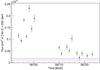 |
Fig. 1 1ES 1011+496 light curve between February 6th and March 7th 2014 above an energy threshold of 200 GeV with a night-wise binning. The blue dashed line indicates the mean integral flux for the MAGIC observations of 2007 and the red dotted line the MWL campaign between 2011 and 2012. |
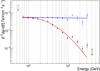 |
Fig. 2 Spectral energy distribution of 1ES 1011+496 for the 17 nights of observations between February 6 and March 7 2014. The black dots are the observed data and the blue triangles are the data after EBL de-absorption. The red line indicates the fit to a broken power law with transition region function of the observed SED, whereas the blue line indicates the fit to a power-law function of the de-absorbed SED. |
The night-wise estimated intrinsic spectra could all be fitted with power laws, and the evolution of the resulting photon indices is shown in Fig. 3. In the latter part of the observed period, the activity of the source was lower, resulting in larger uncertainties for the fits. There is no evidence for significant spectral variability in the period covered by MAGIC observations, despite the large variations in the absolute flux.
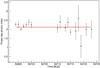 |
Fig. 3 Evolution of the photon index from power-law fits to the de-absorbed night-wise spectra of 1ES 1011+496 between February 6 and March 7 2014. The error bars are the parameter uncertainties from the fits. The red line represents the fit to a constant value, for which the probability is 10%. |
4. EBL constraint
We follow the procedure described in Abramowski et al. (2013) for the likelihood ratio test. The absorption of the EBL is described as e− ατ(E,z), where τ(E,z) is the optical depth predicted by the model, which depends on the energy E of the γ-rays and the redshift z of the source. With the optical depth scaled by a factor α, the observed spectrum is formed as 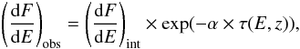 (3)where (dF/ dE)int is the intrinsic spectrum of the source. The emission of HBLs, like 1ES 1011+496, is often well described by basic synchrotron self-Compton (SSC) models (e.g. Tavecchio et al. 1998). A population of electrons is accelerated to ultrarelativistic energies with a resulting power-law spectrum with index Γe of about 2. The high energy electrons are cooled faster than the low energy ones, resulting in a steeper Γe. These electrons produce synchrotron radiation with a photon index
  . In the Thomson regime, the energy spectrum index of the inverse-Compton scattered photons is approximately the same as the synchrotron energy spectrum, whereas in the Klein-Nishima regime, the resulting photon index is even larger. These arguments put serious constraints to the photon index of the energy spectrum of VHE photons. Additionally, in most of the SSC models, the emission is assumed to be originated in a single compact region, which results in a smooth SED with two concave peaks. The shape of the individual peaks could be modified in a multizone model, where the emission is a superposition of several one-zone emission regions. However the general two-peak structure is conserved.
For the modeling of the intrinsic source spectrum, we used the same functions as in Mazin & Raue (2007) and Abramowski et al. (2013) which were also used to fit the observed spectrum: PWL, LP, EPWL, ELP, and SEPWL. We added the additional constraint that the shapes cannot be convex, i.e. the hardness of the spectrum cannot increase with energy since this is not expected in emission models, nor has it been observed in any BL Lac in the optically-thin regime. In particular, the un-absorbed part of BL Lac spectra, measured by Fermi-LAT, are well fitted by log parabolas (Ackermann et al. 2012).
The PWL and the LP are functions that are linear in their parameters in the log flux–log E representation (hence well-behaved in the fitting process), and both can model pretty well the de-absorbed spectrum found in Sect. 3. The EPWL, ELP, and SEPWL have additional (non-linear) parameters that are physically motivated, e.g. to account for possible internal absorption at the source. We note that these functions (except the PWL) can also mimic the overall spectral curvature induced by the EBL over a wide range of redshifts, but will be unable to fit the inflection point (in the optical depth vs. log E curvature) that state-of-the-art EBL models predict around 1 TeV. We therefore expect an improvement of the fit quality as we approach the true value of the scaling factor α, hence providing a constraint of the actual EBL density. The chosen spectral functions, however, do not exhaust all possible concave shapes. Therefore the EBL constraints that we obtain are valid under the assumption that the true intrinsic spectrum can be well described (within the uncertainties of the recorded fluxes) by one of those functions. As we saw in Sect. 3, the 5-parameter SBPWL (not included among the possible spectral models) provides an acceptable fit to the observed spectrum; if considered a plausible model for the intrinsic spectrum, it would severely weaken the lower EBL density constraint. On the contrary, the upper constraint (arguably the most interesting one that VHE observations can contribute) from this work would be unaffected, as we see below.
To search for the imprint of the EBL on the observed spectrum, a scan over α was computed, varying the value from 0 to 2.5. In each step of the scan, the model for the intrinsic spectrum was modified using the EBL model by Domínguez et al. (2011), with the scaled optical depth using the expression (3) and then was passed through the response of the MAGIC telescopes (accounting for the effective area of the system, energy reconstruction, observation time). Then the Poissonian likelihood of the actual observation (the post-cuts number of recorded events vs. Eest, in both the ON and OFF regions) was computed, after maximizing it in a parameter space which includes, besides the intrinsic spectral parameters, the Poisson parameters of the background in each bin of Eest1. The maximum likelihood was thus obtained for each value of alpha. This likelihood shows a maximum at a value α = α0, which indicates that the EBL opacity scaling achieves a best fit to the data. A likelihood ratio test was then performed to compare the no-EBL hypothesis (α = 0) with the best-fit EBL hypothesis (α = α0). The test statistics TS = 2log (ℒ(α = α0/ ℒ(α = 0)), according to Wilks’ theorem, asymptotically follows a χ2 distribution with one degree of freedom (since the two hypotheses differ by just one free parameter, α).
Despite changing the flux level, the EBL determination method should work properly as long as the average intrinsic spectrum in the observation period can be described with one of the tested parameterizations. Assuming that is the case for the different states of the source, it should also hold for the average spectrum if the spectral shape is stable through the flare. A simple way to check the stability of the spectral shape is fitting the points on Fig. 3 to a constant value. The χ2/d.o.f. of this fit is 23.5 / 16 and the probability is 10%, so there is no clear signature of spectral variability – beyond a weak hint of harder spectra in the second half of the observation period. A varying spectral shape would, in any case, need a significant amount of fine-tuning to reproduce, in the average spectrum, a feature like the one expected to be induced by the EBL.
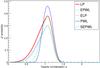 |
Fig. 4 χ2 probability distributions for the average spectrum of the February–March flare of 1ES 1011+496 for the five models tested. PWL in blue (dashed line), LP in red (solid line), EPWL in green (dash-dot line), ELP in pink (dotted line), and SEPWL in light blue (long dash-dot line). |
χ2 probabilities (P) for the cases of α = 0.0 and α = 1.07.
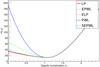 |
Fig. 5 Fit χ2 distributions for the average spectrum of the February–March flare of 1ES 1011+496 for the five models tested. PWL in blue (dashed line), LP in red (solid line), EPWL in green (dot-dash line) and ELP in pink (dotted line) and SEPWL in light blue (long dash-dot line). The LP red line is overlapping ELP pink line. Notice how all curves converge after reaching the minimum. |
Figure 4 shows the χ2 probabilities for the five tested models, also listed in Table 1, for the no-EBL case (α = 0.0) and the best-fit α = 1.07. The model that gives the highest probability in the scanned range of α is the PWL. Following the approach in Abramowski et al. (2013) would lead us to choose the PWL as model for the intrinsic spectrum, as the next models in complexity (LP and EPWL) are not preferred at the 2σ level. However, choosing a PWL as the preferred model is rather questionable since it would not allow any intrinsic spectral curvature, meaning that all curvature in the observed spectrum will be attributed to the EBL absorption. If this procedure is applied to a large number of spectra, as in Biteau & Williams (2015), individual <2σ hints of intrinsic (concave) curvature might be overlooked and accumulate to produce a bias in the EBL estimation. In our case, the assumption of power-law intrinsic spectrum for 1ES 10111+496 would lead the likelihood ratio test to prefer the best-fit α value to the no-EBL hypothesis by as much as 13σ. We prefer to adopt a more conservative approach, choosing the next-best function, the LP. We note however that, at the best-fit α, all the tested functions become simple power laws, hence the fit probabilities at the peak depend only on the number of free parameters. At the best-fit α = 1.07, the parameters of the PWL are: photon index Γ = 1.9 ± 0.1 and normalisation factor at 250 GeV f0 = (9.2 ± 0.2) × 10-10 cm-2 s-1 TeV-1. The other functions have the same values for these parameters.
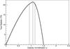 |
Fig. 6 Test statistics distribution for the data sample for the February–March 2014 flare of 1ES 1011+496. The vertical lines mark the maximum and the uncertainty corresponding to 1σ. |
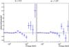 |
Fig. 7 Ratio between the observed events and the expected events from the model of the intrinsic spectrum for two normalization values of the EBL optical depth, α = 0 to the left and α = 1.07 to the right, which corresponds to the normalization where the maximum TS was found. In both plots, the line that correspond to a ratio = 1 is shown. |
Going deeper in the behaviour of the fits for the five models, it can be seen in Fig. 5 that, after reaching the minimum, the χ2 are identical for all models. This happens because of the concavity restriction imposed to the functions. After reaching the point where the EBL de-absorption results in a straight power-law intrinsic spectrum, all three functions converge and the de-absorbed spectra become more and more convex as α increases (so no concave function can fit it any better than a simple power law). The shape of the spectrum observed by MAGIC is thus very convenient for setting upper bounds to the EBL density, under the adopted assumption that convex spectra are “unphysical”.
Given these arguments, we take the LP as our model for the intrinsic spectrum. For the data sample from the 2014 February–March flare of 1ES 1011+496, the test statistic has a maximum of TS = 21.5 at  (Fig. 6). This means that the EBL optical depth from the model of Domínguez et al. (2011), scaled by the normalization factor α0, is preferred over the null EBL hypothesis with a significance of 4.6σ. Using the EBL model of Franceschini et al. (2008) as a template (as in Abramowski et al. 2013), the test statistic has a maximum of TS = 20.6 at
  , using the LP as a model for the intrinsic spectrum, which is compatible with the result when using Domínguez et al. (2011) within statistical uncertainty.
We again note that allowing for other concave spectral shapes, like the SBPWL, would severely affect our lower EBL bound. This would also be the case for earlier published EBL lower constraints that are based on gamma-ray data – especially those in which the PWL is among the allowed models for the intrinsic spectrum. For the observations discussed in the present paper, the SBPWL would achieve an acceptable fit even in the no-EBL assumption. This and earlier constraints on the EBL density, through its imprint on γ-ray spectra, therefore rely on somewhat tentative assumptions on the intrinsic spectra – assumptions which, as far as we know, are not falsified by any observational data available on BL Lacs. On the other hand, the upper bound we obtained is robust since it is driven by the fact that convex spectral shapes (completely unexpected for BL Lacs at VHE) would be needed to fit our observations, if EBL densities above the best-fit value are assumed.
5. Systematic uncertainty
The MAGIC telescopes has a systematic uncertainty in the absolute energy scale of 15% (Aleksić et al. 2015b). The main source of this uncertainty is the imprecise knowledge of the atmospheric transmission. To assess how this uncertainty affects the EBL constraint, the calibration constants used to convert the pixel-wise digitized signals into photoelectrons were multiplied by a scaling factor (the same for both telescopes) spanning the range –15% to +15% in steps of 5%. This procedure is similar as the one presented by Aleksić et al. (2015b).
For each of the scaling factors, the data were processed in an identical manner through the full analysis chain, starting from the image cleaning and using, in all cases, the standard MAGIC MC for this observation period. In this way, we try to asses the effect of a potential miscalibration between the data and the MC simulation.
For all scaled data samples, χ2 profiles for α between 0 and 2.5 were computed. From the 1σ uncertainty ranges in α obtained for the different shifts in the light scale, we determine the largest departures from our best-fit value α0, arriving to the final result α0 = 1.07 (–0.20, +0.24)stat+sys.
6. Discussion
The relation of the γ-ray of energy Eγ from the source (measured in the observed frame) and the EBL wavelength at the peak of the cross section for the photon-photon interaction is given by  (4)where z is equal or less than the redshift of the source. The energy range used for our calculations was between 0.06 and 3.5 TeV. However, the constraining of the EBL, following the method from Abramowski et al. (2013), is based on the fact that, after de-absorbing the EBL effect, the feature between ~100 GeV and ~5–10 TeV is suppressed. In Fig. 7, we show a comparison between two cases where the residuals were computed (the ratio between the observed events and the expected events from the model). The plot on the left shows the residuals for the null EBL hypothesis α = 0, while the right pad shows the same plot for the case of the best fit EBL scaling α = 1.07. The differences start to show after 200 GeV, a region where the EBL introduces a feature (an inflection point) that cannot be fitted by the log parabola. This is the feature that drives the TS value on which the EBL constraint is based. We therefore calculate the EBL wavelength range for which our conclusion is valid from the VHE range between 0.2 and 3.5 TeV.
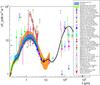
The energy range has to take into account the redshift dependency in Eq. (4) since the interaction of the γ-ray and the EBL photons can happen in any point between the Earth and the source. The range is between [(1 + z)2Emin,Emax], corresponding to a wavelength range of the EBL where the interaction with the γ-ray can take place along the entire path between the source and the Earth. In Fig. 8, we show the contours from the statistical + systematic uncertainty of the EBL flux density, which was derived by scaling up the EBL template model by Domínguez et al. (2011) at redshift z = 0. The wavelength coverage is in the so-called cosmic optical background (COB) part of the EBL where we found the peak flux density  nW m-2 sr-1 at 1.4 μm, systematics included.
7. Conclusions
We have reported the observation of the extraordinary outburst from 1ES 1011+496 that were observed by MAGIC from February 6 to March 7 2014 when the flux reached a level ~14 times the observed flux at the time of the discovery of the source in 2007. During this flare, the spectrum of 1ES 1011+496 displays little intrinsic curvature over >1 order of magnitude in energy, which makes this an ideal observation for constraining the EBL. Although the source showed a high flux variability during the observed period, no significant change of the spectral shape was observed during the flare, which enabled us to use the average observed spectrum in the search for an imprint of the EBL-induced absorption of γ rays on it. This type of EBL imprint can be seen in the fit residuals of the best fit that was achieved under the no-EBL assumption (Fig. 7, left). In the approach that we followed throughout this work, we restricted ourselves to smooth concave functions for the description of the intrinsic spectrum at VHE which, in the past have provided good fits to BL Lac spectra whenever the expected EBL absorption was negligible. Under this assumption, the best-fit EBL density at λ = 1.4 μm is nW m-2 sr-1, which ranks among the strongest EBL density constraints obtained from VHE data of a single source.
Note that, in the Poissonian likelihood approach, we have included the point at E ~ 55 GeV, which was shown as just an upper limit in Fig. 2, since it has an excess of around just one standard deviation above the background. The fit performed with the Poissonian likelihood approach has therefore one more degree of freedom than the χ2 fits reported in Sect. 3 and the 55 GeV point is included in Fig. 7.
Acknowledgments
We would like to thank the Instituto de Astrofísica de Canarias for the excellent working conditions at the Observatorio del Roque de los Muchachos in La Palma. The financial support of the German BMBF and MPG, the Italian INFN and INAF, the Swiss National Fund SNF, the ERDF under the Spanish MINECO, and the Japanese JSPS and MEXT is gratefully acknowledged. This work was also supported by the Centro de Excelencia Severo Ochoa SEV-2012-0234, CPAN CSD2007-00042, and MultiDark CSD2009-00064 projects of the Spanish Consolider-Ingenio 2010 programme, by grant 268740 of the Academy of Finland, by the Croatian Science Foundation (HrZZ) Project 09/176 and the University of Rijeka Project 13.12.1.3.02, by the DFG Collaborative Research Centers SFB823/C4 and SFB876/C3, and by the Polish MNiSzW grant 745/N-HESS-MAGIC/2010/0. We thank the anonymous referee for a thorough review and a very constructive list of remarks that helped to improve the quality and clarity of this manuscript.
References
- Abramowski, A., Acero, F., Aharonian, A. G., H.E.S.S. Collaboration, et al. 2013, A&A, 550, A4 [NASA ADS] [CrossRef] [EDP Sciences] [Google Scholar]
- Ackermann, M., Ajello, M., Allafort, A., et al. 2012, Science, 338, 1190 [NASA ADS] [CrossRef] [Google Scholar]
- Aharonian, F., Akhperjanian, A. G., Bazer-Bachi, A. R., et al. 2006, Nature, 440, 1018 [NASA ADS] [CrossRef] [PubMed] [Google Scholar]
- Ahnen, M. L., Ansoldi, S., Antonelli, L. A., et al. 2016, MNRAS, accepted [arXiv:1603.07308] [Google Scholar]
- Albert, J., Aliu, E., Anderhub, H., et al. 2007, ApJ, 667, L21 [NASA ADS] [CrossRef] [Google Scholar]
- Aleksić, J., Ansoldi, S., Antonelli, L. A., et al. 2015a, APh, in press [Google Scholar]
- Aleksić, J., Ansoldi, S., Antonelli, L. A., et al. 2015b, APh, in press [Google Scholar]
- Aleksić, J., Ansoldi, S., Antonelli, L. A., et al. 2016, A&A, accepted [arXiv:1603.06776] [Google Scholar]
- Berta, S., Magnelli, B., Lutz, D., et al. 2010, A&A, 518, L30 [NASA ADS] [CrossRef] [EDP Sciences] [Google Scholar]
- Béthermin, M., Dole, H., Beelen, A., & Aussel, H. 2010, A&A, 512, A78 [NASA ADS] [CrossRef] [EDP Sciences] [Google Scholar]
- Biteau, J., & Williams, D. A. 2015, ApJ, 812, 60 [NASA ADS] [CrossRef] [Google Scholar]
- Brown, T. M., Kimble, R. A., Ferguson, H. C., et al. 2000, AJ, 120, 1153 [NASA ADS] [CrossRef] [Google Scholar]
- Cambrésy, L., Reach, W. T., Beichman, C. A., & Jarrett, T. H. 2001, ApJ, 555, 563 [NASA ADS] [CrossRef] [Google Scholar]
- Cooray, A., Bock, J. J., Keatin, B., Lange, A. E., & Matsumoto, T. 2004, ApJ, 606, 611 [NASA ADS] [CrossRef] [Google Scholar]
- Dole, H., Rieke, G. H., Lagache, G., et al. 2004, ApJS, 154, 93 [NASA ADS] [CrossRef] [Google Scholar]
- Dole, H., Lagache, G., Puget, J.-L., et al. 2006, A&A, 451, 417 [NASA ADS] [CrossRef] [EDP Sciences] [MathSciNet] [Google Scholar]
- Domínguez, A., Finke, J. D., Prada, F., et al. 2013, ApJ, 770, 77 [NASA ADS] [CrossRef] [Google Scholar]
- Domínguez, A., Primack, J. R., Rosario, D. J., et al. 2011, MNRAS, 410, 2556 [NASA ADS] [CrossRef] [Google Scholar]
- Dube, R. R., Wickes, W. C., & Wilkinson, D. T. 1979, ApJ, 232, 333 [NASA ADS] [CrossRef] [Google Scholar]
- Dwek, E., & Arendt, R. G. 1998, ApJ, 508, L9 [NASA ADS] [CrossRef] [Google Scholar]
- Edelstein, J., Bowyer, S., & Lampton, M. 2000, ApJ, 539, 187 [NASA ADS] [CrossRef] [Google Scholar]
- Elbaz, D., Flores, H., Chanial, P., et al. 2002, A&A, 381, L1 [NASA ADS] [CrossRef] [EDP Sciences] [Google Scholar]
- Fazio, G. G. 2005, Neutrinos and Explosive Events in the Universe, 47 [Google Scholar]
- Fazio, G. G., Ashby, M. L. N., Barmby, P., et al. 2004, ApJS, 154, 39 [NASA ADS] [CrossRef] [Google Scholar]
- Fernandez, E. R., Komatsu, E., Iliev, I. T., & Shapiro, P. R. 2010, ApJ, 710, 1089 [NASA ADS] [CrossRef] [Google Scholar]
- Finkbeiner, D. P., Davis, M., & Schlegel, D. J. 2000, ApJ, 544, 81 [NASA ADS] [CrossRef] [Google Scholar]
- Finke, J. D., Razzaque, S., & Dermer, C. D. 2010, ApJ, 712, 238 [NASA ADS] [CrossRef] [Google Scholar]
- Fomin, V. P., Stepanian, A. A., Lamb, R. C., et al. 1994, Astropart. Phys., 2, 137 [NASA ADS] [CrossRef] [Google Scholar]
- Franceschini, A., Rodighiero, G., & Vaccari, M. 2008, A&A, 837, 487 [Google Scholar]
- Frayer, D. T., Huynh, M. T., Chary, R., et al. 2006, ApJ, 647, L9 [NASA ADS] [CrossRef] [Google Scholar]
- Gardner, J. P., Brown, T. M., & Ferguson, H. C. 2000, ApJ, 542, L79 [NASA ADS] [CrossRef] [Google Scholar]
- Georganopoulos, M., Finke, J. D., & Reyes, L. C. 2010, ApJ, 714, L157 [NASA ADS] [CrossRef] [Google Scholar]
- Gorjian, V., Wright, E. L., & Chary, R. R. 2000, ApJ, 536, 550 [NASA ADS] [CrossRef] [Google Scholar]
- Gould, R. J., & Schréder, G. P. 1967, Phys. Rev., 155, 1408 [NASA ADS] [CrossRef] [Google Scholar]
- Hauser, M. G., & Dwek, E. 2001, ARA&A, 39, 249 [NASA ADS] [CrossRef] [Google Scholar]
- Hauser, M. G., Arendt, R. G., Kelsall, T., et al. 1998, ApJ, 508, 25 [NASA ADS] [CrossRef] [Google Scholar]
- Kashlinsky, A., Mather, J. C., Odenwald, S., & Hauser, M. G. 1996, ApJ, 470, 681 [NASA ADS] [CrossRef] [Google Scholar]
- Keenan, R. C., Barger, A. J., Cowie, L. L., & Wang, W.-H. 2010, ApJ, 723, 40 [NASA ADS] [CrossRef] [Google Scholar]
- Krick, J. E., & Bernstein, R. A. 2005, Am. Astron. Soc. Meet. Abstr., 37, 177.14 [Google Scholar]
- Lagache, G., Haffner, L. M., Reynolds, R. J., & Tufte, S. L. 2000, A&A, 354, 247 [Google Scholar]
- Levenson, L. R., & Wright, E. L. 2008, ApJ, 683, 585 [NASA ADS] [CrossRef] [Google Scholar]
- Levenson, L. R., Wright, E. L., & Johnson, B. D. 2007, ApJ, 666, 34 [NASA ADS] [CrossRef] [Google Scholar]
- Li, T., & Ma, Y. 1983, ApJ, 317 [Google Scholar]
- Madau, P., & Pozzetti, L. 2000, MNRAS, 312, L9 [NASA ADS] [CrossRef] [Google Scholar]
- Mankuzhiyil, N., Persic, M., & Tavecchio, F. 2010, ApJ, 715, L16 [NASA ADS] [CrossRef] [Google Scholar]
- Martin, P. G., & Rouleau, F. 1991, in Extreme Ultraviolet Astronomy, A Selection of Papers Presented at the First Berkeley Colloquium on Extreme Ultraviolet Astronomy, University of California, Berkeley, January 19–20, 1989, eds. R. F. Malina, & S. Bowyer (New York: Pergamon Press) [Google Scholar]
- Matsumoto, T., Kim, M. G., Pyo, J., & Tsumura, K. 2015, ApJ, 807, 57 [NASA ADS] [CrossRef] [Google Scholar]
- Matsumoto, T., Matsuura, S., Murakami, H., et al. 2005, ApJ, 626, 31 [NASA ADS] [CrossRef] [Google Scholar]
- Matsuoka, Y., Ienaka, N., Kawara, K., & Oyabu, S. 2011, ApJ, 736, 119 [NASA ADS] [CrossRef] [Google Scholar]
- Mattila, K., et al. 1991, The Early Observable Universe from Diffuse Backgrounds, 133 [Google Scholar]
- Mazin, D., & Raue, M. 2007, A&A, 471, 439 [NASA ADS] [CrossRef] [EDP Sciences] [Google Scholar]
- Metcalfe, L., Kneib, J.-P., McBreen, B., et al. 2003, A&A, 407, 791 [NASA ADS] [CrossRef] [EDP Sciences] [MathSciNet] [Google Scholar]
- Meyer, M., Raue, M., Mazin, D., & Horns, D. 2012, A&A, 542, A59 [NASA ADS] [CrossRef] [EDP Sciences] [Google Scholar]
- Orr, M. R., Krennrich, F., & Dwek, E. 2011, ApJ, 733, 77 [NASA ADS] [CrossRef] [Google Scholar]
- Papovich, C., Dole, H., Egami, E., et al. 2004, ApJS, 154, 70 [NASA ADS] [CrossRef] [Google Scholar]
- Pénin, A., Lagache, G., Noriega-Crespo, A., et al. 2012, A&A, 543, A123 [NASA ADS] [CrossRef] [EDP Sciences] [Google Scholar]
- Reinthal, R., Rügamer, S., Lindfors, E. J., et al. 2012, J. Phys. Conf. Ser., 355, 012017 [NASA ADS] [CrossRef] [Google Scholar]
- Stecker, F. W., & de Jager, O. C. 1996, Space Sci. Rev., 75, 401 [NASA ADS] [CrossRef] [Google Scholar]
- Stecker, F. W., Malkan, M. A., & Scully, S. T. 2006, ApJ, 774 [NASA ADS] [CrossRef] [Google Scholar]
- Tavecchio, F., Maraschi, L., & Ghisellini, G. 1998, ApJ, 509, 608 [NASA ADS] [CrossRef] [Google Scholar]
- Thompson, R. I., Eisenstein, D., Fan, X., Rieke, M., & Kennicutt, R. C. 2007, ApJ, 657, 669 [NASA ADS] [CrossRef] [Google Scholar]
- Voyer, E. N., Gardner, J. P., Teplitz, H. I., Siana, B. D., & de Mello, D. F. 2011, ApJ, 736, 80 [NASA ADS] [CrossRef] [Google Scholar]
- Weekes, T. C., Badran, H., Biller, S. D., et al. 2002, Astropart. Phys., 17, 221 [Google Scholar]
- Wright, E. L. 2001, ApJ, 553, 538 [Google Scholar]
- Xu, C. K., Donas, J., Arnouts, S., et al. 2005, ApJ, 619, L11 [NASA ADS] [CrossRef] [Google Scholar]
- Zanin, R., Carmona, E., Sitarek, J., et al. 2013, Proc of the 33rd ICRC, Rio de Janeiro, 2 [Google Scholar]
- Zemcov, M., Smidt, J., Arai, T., et al. 2014, Science, 346, 732 [NASA ADS] [CrossRef] [Google Scholar]
All Tables
All Figures
|
Fig. 1 1ES 1011+496 light curve between February 6th and March 7th 2014 above an energy threshold of 200 GeV with a night-wise binning. The blue dashed line indicates the mean integral flux for the MAGIC observations of 2007 and the red dotted line the MWL campaign between 2011 and 2012. |
| In the text | |
|
Fig. 2 Spectral energy distribution of 1ES 1011+496 for the 17 nights of observations between February 6 and March 7 2014. The black dots are the observed data and the blue triangles are the data after EBL de-absorption. The red line indicates the fit to a broken power law with transition region function of the observed SED, whereas the blue line indicates the fit to a power-law function of the de-absorbed SED. |
| In the text | |
|
Fig. 3 Evolution of the photon index from power-law fits to the de-absorbed night-wise spectra of 1ES 1011+496 between February 6 and March 7 2014. The error bars are the parameter uncertainties from the fits. The red line represents the fit to a constant value, for which the probability is 10%. |
| In the text | |
|
Fig. 4 χ2 probability distributions for the average spectrum of the February–March flare of 1ES 1011+496 for the five models tested. PWL in blue (dashed line), LP in red (solid line), EPWL in green (dash-dot line), ELP in pink (dotted line), and SEPWL in light blue (long dash-dot line). |
| In the text | |
|
Fig. 5 Fit χ2 distributions for the average spectrum of the February–March flare of 1ES 1011+496 for the five models tested. PWL in blue (dashed line), LP in red (solid line), EPWL in green (dot-dash line) and ELP in pink (dotted line) and SEPWL in light blue (long dash-dot line). The LP red line is overlapping ELP pink line. Notice how all curves converge after reaching the minimum. |
| In the text | |
|
Fig. 6 Test statistics distribution for the data sample for the February–March 2014 flare of 1ES 1011+496. The vertical lines mark the maximum and the uncertainty corresponding to 1σ. |
| In the text | |
|
Fig. 7 Ratio between the observed events and the expected events from the model of the intrinsic spectrum for two normalization values of the EBL optical depth, α = 0 to the left and α = 1.07 to the right, which corresponds to the normalization where the maximum TS was found. In both plots, the line that correspond to a ratio = 1 is shown. |
| In the text | |
Current usage metrics show cumulative count of Article Views (full-text article views including HTML views, PDF and ePub downloads, according to the available data) and Abstracts Views on Vision4Press platform.
Data correspond to usage on the plateform after 2015. The current usage metrics is available 48-96 hours after online publication and is updated daily on week days.
Initial download of the metrics may take a while.