| Issue |
A&A
Volume 627, July 2019
|
|
|---|---|---|
| Article Number | A110 | |
| Number of page(s) | 12 | |
| Section | Astrophysical processes | |
| DOI | https://doi.org/10.1051/0004-6361/201834240 | |
| Published online | 09 July 2019 | |
Normalization of the extragalactic background light from high-energy γ-ray observations
1
Institut de Physique Nucléaire, IN2P3/CNRS, Université Paris-Sud, Univ. Paris/Saclay, 15 rue Georges Clémenceau, 91406 Orsay, Cedex, France
e-mail: This email address is being protected from spambots. You need JavaScript enabled to view it.
2
Santa Cruz Institute for Particle Physics and Department of Physics, University of California at Santa Cruz, Santa Cruz, CA 95064, USA
Received:
13
September
2018
Accepted:
3
June
2019
Abstract
Extragalactic background light (EBL) plays an important role in cosmology since it traces the history of galaxy formation and evolution. Such diffuse radiation from near-UV to far-infrared wavelengths can interact with γ-rays from distant sources such as active galactic nuclei (AGNs), and is responsible for the high-energy absorption observed in their spectra. However, probing the EBL from γ-ray spectra of AGNs is not trivial due to internal processes that can mimic its effect. Such processes are usually taken into account in terms of curvature of the intrinsic spectrum. Hence, an improper choice of parametrization for the latter can seriously affect EBL reconstruction. In this paper, we propose a statistical approach that avoids a priori assumptions on the intrinsic spectral curvature and that, for each source, selects the best-fit model on a solid statistical basis. By combining the Fermi-LAT observations of 490 blazars, we determine the γ-ray-inferred level of EBL for various state-of-the-art EBL models. We discuss the EBL level obtained from the spectra of both BL Lacs and flat spectrum radio quasars (FSRQ) in order to investigate the impact of internal absorption in different classes of objects. We further scrutinize constraints on the EBL evolution from γ-ray observations by reconstructing the EBL level in four redshift ranges, up to z ∼ 2.5. The approach implemented in this paper, carefully addressing the question of the modeling of the intrinsic emission at the source, can serve as a solid stepping stone for studies of hundreds of high-quality spectra acquired by next-generation γ-ray instruments.
Key words: astroparticle physics / galaxies: active / cosmology: observations / diffuse radiation / gamma rays: galaxies
© B. Biasuzzi et al. 2019
 Open Access article, published by EDP Sciences, under the terms of the Creative Commons Attribution License (http://creativecommons.org/licenses/by/4.0), which permits unrestricted use, distribution, and reproduction in any medium, provided the original work is properly cited.
1. Introduction
The extragalactic background light (EBL) is the brightest background photon field after the cosmic microwave background (CMB) radiation. Its spectrum, which ranges from 0.1 to 1000 μm, is formed by the contribution of stars and accreting compact objects during the whole history of the universe. The direct light emitted in the UV and optical bands builds up the so-called cosmic optical background (COB), peaking around λ ∼ 1 μm, while the light reprocessed by dust close to the emitter and in the interstellar medium contributes to the cosmic infrared background (CIB), peaking around λ ∼ 100 μm (Dwek & Krennrich 2013). The EBL spectrum is hard to measure directly because of the presence of strong foreground emissions, such as the zodiacal light and the light emitted by the Galactic plane, and therefore direct sky photometry usually provides an overestimation of the EBL and leads to large uncertainties (Hauser & Dwek 2001). On the other hand, lower limits on the EBL spectrum can be obtained by summing up the light emitted by resolved sources. However, this approach is affected by the limited sensitivity of the surveys used, which can result in missing objects (Levenson & Wright 2008; Madau & Pozzetti 2000; Dole et al. 2006), although convergence is now observed in a number of bands (Driver et al. 2016).
Knowledge of the evolution of the EBL density is fundamental to understanding the history of galaxy formation and evolution, the stellar initial mass function, the metallicity evolution, and all the processes in the universe related to thermal energy release. However, local measurements of the EBL spectrum do not provide any information about its evolution with cosmic epochs, and therefore various approaches have been followed to model the EBL density as a function of redshift, z. The so-called empirical models, starting from present galaxy luminosity functions of different populations, aim to reconstruct them back in time by assuming a z-dependence inferred by fitting the model prediction to the observed galaxy counts (Stecker & Scully 2006; Franceschini et al. 2008; Domínguez et al. 2011; Franceschini & Rodighiero 2017, 2018). On the contrary, in phenomenological models, the EBL density is obtained by modeling the emission processes throughout galaxy formation and evolution in the universe. Such approaches (Dwek & Arendt 1998; Razzaque et al. 2009; Finke et al. 2010) combine the z-dependence of the star formation rate and different models of population synthesis to obtain the luminosity density at different redshifts. Finally, semi-analytic models (e.g., Gilmore et al. 2012) predict the evolving EBL out to high redshifts using cosmological simulations and incorporating all the most important physical processes that determine galaxy evolution. The derived predictions of such models are then compared to observational quantities such as galaxy morphology, color, spectral energy distribution (SED), and counts. Deriving phenomenological and semi-analytic models is challenging because such models involve several astrophysical processes, sometimes poorly constrained, but they still remain the most physically motivated models with respect to the empirical ones.
Another way to carry out studies of the EBL is through observations of high-energy spectra of distant sources, such as active galactic nuclei (AGNs). In particular, blazars, AGNs whose relativistic jets point directly towards the observer, are the best candidates. They are among the most powerful γ-ray sources in the sky since their luminosity is amplified by a relativistic boosting of a factor ∼δ4, where δ ∼ 𝒪(10) is the Doppler factor of the source. Blazars are characterized by strongly variable nonthermal emission, whose SED shows two peaks: one located at low energies (from infrared to X-rays) that is thought to arise from synchrotron emission, and one located at high energies (in the MeV–TeV range) that is usually interpreted – in leptonic scenarios – as inverse-Compton scattering of relativistic electrons on local photon fields (Band & Grindlay 1985; Tavecchio et al. 1998; Sikora et al. 2008). On the other hand, in hadronic scenarios (Mannheim 1993; Aharonian 2000), a protonic component in the jet would contribute to the high-energy peak, especially via proton synchrotron or via the decay of neutral pions on top of inverse-Compton emission. The characteristic observed high-energy spectrum has a smooth and concave shape (i.e., downward sloping). A further cutoff in the spectrum is expected if one of the following processes takes places: intrinsic self-absorption, Klein-Nishina suppression, cut-off in the parent population of accelerated particles, or EBL absorption.
The presence of blazars in a wide redshift range makes them ideal candidates to study the EBL evolution with cosmic epochs. Before reaching the observer, some of the γ-rays emitted by blazars interact with EBL photons, generating electron–positron pairs (Nikishov 1962; Gould & Schréder 1967). This interaction results in a flux decrease at very-high energies (VHE, E > 100 GeV), a feature that led several authors to attempt to constrain the EBL from the absorbed region in blazar spectra. Even if this technique is independent from direct measurements, it is limited by the fact that the intrinsic emission processes at play in blazars are still not very well understood. Upper limits on the EBL have been estimated by assuming a maximum hardness of AGN spectra in the γ-ray band (Stecker et al. 1992; Mazin & Raue 2007; Finke & Razzaque 2009), or by assuming no intrinsic curvature at all (Meyer et al. 2012; Sinha et al. 2014).
The Fermi-LAT and the H.E.S.S. collaborations proposed an approach to measure the EBL, where the EBL absorption is scaled by a normalizing factor, α, that indicates the agreement between a given EBL model and the γ-ray data (Ackermann et al. 2012; H.E.S.S. Collaboration 2013). By combining observations of several blazars and making minimal assumptions on the intrinsic spectra, they derived the scaling factor for different EBL models.
The pair creation process depends both on the energy of the photons and the redshift of the source. A γ-ray of energy E can interact with EBL photons up to λmax ∼ 2.4 μm (E0/500 GeV)(1 + z)2, as imposed by the energy threshold of the process. This means that ground- and space-based γ-ray observations can explore different regions of the EBL spectrum depending on the γ-ray energy range and redshift they cover. The Fermi-LAT Collaboration (Ackermann et al. 2012) explored the COB peak of the EBL spectrum by using 150 blazar spectra in the redshift range 0 < z < 1.6. The H.E.S.S. Collaboration (H.E.S.S. Collaboration 2013) used 17 blazar spectra up to z < 0.2 to probe the EBL spectrum from 0.30 to 17 μm. In both approaches, a likelihood maximization is performed over the scaling factor in order to compare the best-fit case with the null hypothesis, α = 0 (i.e., absence of EBL absorption), which was rejected at the 6σ level in the Fermi work, and 9σ in the H.E.S.S. one.
By following a similar approach to Ackermann et al. (2012) and H.E.S.S. Collaboration (2013), Ahnen et al. (2015) and Abeysekara et al. (2015) placed constraints on the EBL in a different energy range using observations of PKS 1441+25, the second-most distant VHE flat spectrum radio quasar (FSRQ) located at z = 0.939 during a high-activity state. In Ahnen et al. (2016a), both MAGIC and Fermi-LAT data of the gravitationally lensed blazar B2 018+357 (the most distant VHE one at z = 0.954) were combined to obtain EBL constraints from 0.3 to 1.1 μm. In Ahnen et al. (2016b), a flaring state of the BL Lac 1ES 1011+496 allowed the MAGIC Collaboration to explore the EBL density between 0.24 μm and 4.25 μm. Finally, Mazin et al. (2017) extended the method used in Ahnen et al. (2016b) to 30 independent energy spectra, derived from eight BL Lacs and four FSRQs, to derive the scaling factor of the EBL in the redshift range 0.031 < z < 0.944 for the EBL model of Domínguez et al. (2011).
Armstrong et al. (2017) analyzed the Fermi-LAT spectra of 16 high-redshift sources (0.847 ≤ z ≤ 1.596) by following the approach of Ackermann et al. (2012). After extrapolating the intrinsic spectra from their unabsorbed region (where the absorption is less than 0.1%), they fit the whole spectrum to derive the EBL level.
The most extensive VHE γ-ray study on the EBL was carried out by Biteau & Williams (2015). They used 86 spectra (from 29 BL Lac objects with reliable redshifts up to z = 0.287) from ground-based observatories (MAGIC, H.E.S.S., VERITAS, Whipple, ARGO-YBJ, HEGRA, TACTIC, Tibet, and CAT) and from space-based observatories (Fermi-LAT), together with the EBL local constraints reported in Dwek & Krennrich (2013). They investigated the 0.26−105 μm EBL spectrum region, improving also on the method of the Fermi-LAT and H.E.S.S. Collaborations by introducing a model-independent approach. The hypothesis of absence of absorption was rejected at the 11σ level.
The H.E.S.S. Collaboration derived the EBL intensity, independent of a given EBL model, using H.E.S.S. data alone and an approach similar to Biteau & Williams (2015). By using 21 spectra from eight high-frequency-peaked BL Lac objects, they determined the EBL level in four wavebands, from 0.25 to 98.6 μm (H.E.S.S. Collaboration 2017). The EBL measurement that they obtained is preferred to the null hypothesis at the 9.5σ level.
The MAGIC Collaboration (Acciari et al. 2019) used MAGIC and Fermi-LAT data, with 32 γ-ray spectra coming from 12 sources, to reconstruct the EBL normalization in the redshift range 0.03 ≤ z ≤ 0.944. They also constrained the EBL spectrum in the range 0.18–100 μm, reaching a total uncertainty of 20% in the range 0.62–2.24 μm.
Finally, Abdollahi et al. (2018) applied the methodology of Ackermann et al. (2012) to a larger sample of 739 AGNs (419 FSRQs and 320 BL Lacs) from the third catalog of AGNs (3LAC, Ackermann et al. 2015) and the GRB 080916C located at z = 4.35. Abdollahi et al. (2018) reconstructed the EBL intensity from ∼0.1 to ∼4 μm, and the cosmic γ-ray horizon up to a redshift z = 3. Moreover, they used a physical EBL model to infer the optical depth directly from the star formation rate (SFR). The latter was then optimized to reproduce the Fermi-LAT optical depth data, thus constraining the SFR over 90% of the cosmic time.
Another way to probe the EBL, especially at high redshift, consists in using only γ-ray bursts (GRBs) detected by Fermi-LAT, as done in Desai et al. (2017). These latter authors combined 22 GRB observations with redshift in the range 0.15 ≤ z ≤ 4.35, disfavoring the hypothesis of no EBL absorption at the ∼2.8σ level. They obtained constraints on the EBL optical depth for an effective redshift of 1.8.
So far, the results obtained by analyzing the γ-ray spectra of AGNs and GRBs are in good agreement with the local constraints on the EBL.
By following the approach in Ackermann et al. (2012) and Abdollahi et al. (2018), while retaining flexibility as to the shape of each intrinsic γ-ray spectrum as in Biteau & Williams (2015), we determine the scaling factor for different EBL models by analyzing the Fermi-LAT spectra of many blazars. After briefly discussing the impact of the choice of the intrinsic-spectrum model in Sect. 2, the source-selection criteria and the full dataset are presented in Sect. 3. The analysis method is described in Sect. 4. Finally, in Sects. 5 and 6, the results are presented and compared to previous EBL measurements, together with the estimate of systematic uncertainties.
2. Impact of intrinsic-spectrum assumption
So far, all the methods proposed in the literature that use several γ-ray emitters to determine the EBL normalization make a priori assumptions on the intrinsic spectrum of the sources. The lack of unequivocal arguments to prefer one model over another can lead to biases in the EBL reconstruction. Ackermann et al. (2012) modeled the intrinsic blazar spectra with a log-parabola function. First, the intrinsic spectral parameters are determined by fitting the unabsorbed part of the spectrum. The EBL normalization is then reconstructed through a second fit in the whole range (1–500 GeV) by fixing the curvature to the value obtained in the previous fit. The choice of a log-parabola parametrization was validated based on the average of the residuals with respect to the best-fit models, on the spectral fit of well-known blazars with coverage in the GeV–TeV band, and on simulations of blazar broad-band spectra. H.E.S.S. Collaboration (2017) also used log-parabola functions to model intrinsic spectra of blazars. A joint fit on each source was performed to obtain both the best spectral parameters and the EBL normalization, using the full energy range covered by the experiment. Finally, all the results were combined together to determine the final EBL normalization. In Armstrong et al. (2017), the authors used two functions to model the unabsorbed part of the spectra: power-law and log-parabola. A likelihood profile was generated as a function of the EBL normalization, and the log-parabola model was chosen if the Test Statistic (TS) between the two models was larger then 16, the same value adopted by the Fermi-LAT Collaboration to choose a more complex spectral model over a power law in the 3FGL catalog (Acero et al. 2015). In H.E.S.S. Collaboration (2013), the intrinsic spectral model was chosen according to the highest χ2 probability of the fit, among power-law, log-parabola, exponential-cutoff power-law, exponential-cutoff log-parabola, and super-exponential-cutoff power-law models. The intrinsic spectral model was chosen individually for each source, and independently from the value of the EBL normalization where the χ2 probability reaches its maximum. The same approach was used in Mazin et al. (2017), but assuming a log-parabola as the simplest function rather than a power law, which could bias the measurement towards low EBL levels. The same procedure and the same spectral models of Mazin & Raue (2007) were used in Acciari et al. (2019). In this case, the determination of the intrinsic spectra involves a further step. Once a first intrinsic model was chosen for each source according to the highest p-value of the fit and independently from the EBL normalization, α, a preliminary maximum-likelihood fit was performed using all 32 sources. The intrinsic spectral models were then recomputed for all the sources whose models were previously outside the 2σ range around the best α. Finally, in Biteau & Williams (2015), the intrinsic spectral models have been selected iteratively in a joint fit together with the EBL normalization. The modeling function is chosen among power-law, log-parabola, exponential-cutoff power-law, and exponential-cutoff log-parabola models. For a given starting set of initial models, in correspondence to the best EBL normalization, a more complex model is selected if preferred at least at the 2σ level (a threshold commonly adopted in the literature) with respect to a simpler one. This procedure is repeated until convergence of the set of intrinsic models.
The assumptions on the parametrization of the intrinsic curvature may have a strong impact on the EBL reconstruction. A weak disentanglement criterion or an improper choice of the intrinsic models can be responsible for either an over- or underestimation of the EBL normalization. An example is provided in Fig. 1, where the EBL normalization has been determined from the source 3FHL J2253.9+1608 (z = 0.86), whose spectrum has been modeled with a power law, an exponential cutoff power law, a log-parabola, and an exponential cutoff log-parabola, respectively. The best spectral parameters are fit together with the EBL normalization. If the intrinsic spectrum is modeled with a power law or an exponential cutoff power law, the χ2 probability is very low: 6.0 × 10−88 and 6.0 × 10⁻⁷, respectively. By using either a log-parabola or an exponential cutoff log-parabola, the fit is better, with a χ2 probability of 0.33 and 0.19, respectively. Nevertheless, the most-likely EBL normalizations differ a lot: 2.7 for the log-parabola, and zero (i.e., no EBL absorption) for the exponential cutoff log-parabola. The cumulative effect – over a large number of sources – due to an improper choice of the intrinsic spectrum, could seriously affect the EBL reconstruction.
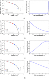 |
Fig. 1. Left panels: 3FHL J2253.9+1608 spectrum, including points from the 3FGL catalog (red), and from 3FHL catalog (blue); upper limits (not included in the fit) are shown in gray. The spectral fit is displayed for the best EBL normalization over the range of interest, and has been performed modeling the intrinsic spectrum with a power law (a), an exponential cutoff power law (b), a log-parabola (c), and an exponential cutoff log-parabola (d). Right panels: likelihood profile as a function of the EBL normalization, α. |
The main aim of this work is to obtain the EBL normalization using an approach that (i) avoids, as much as possible, any assumption on the parametrization of the intrinsic curvature; (ii) justifies the selection criterion among different spectral models; and (iii) determines the best intrinsic spectrum, together with the EBL scaling factor, through a rigorous, joint fitting process. This approach, applied to a blazar sample that combines Fermi-LAT data from two catalogs, is described in Sect. 4, followed by the estimation of the systematic uncertainties in Sect. 5.
3. Data sample
3.1. Source selection
To determine the scaling factor for different EBL models, we used AGN spectra both from the Third Catalog of High-Energy Fermi-LAT Sources (3FHL, Ajello et al. 2017) and the Third Fermi-LAT Source Catalog (3FGL, Acero et al. 2015). The 3FGL catalog compiles data from the first 4 years of the Fermi-LAT mission, for a total of 3033 objects detected above 4σ significance between 100 MeV and 300 GeV, while the 3FHL catalog includes data from 7 years of Fermi-LAT observations, counting 1556 sources detected between 10 GeV and 2 TeV. The 3FHL data have been processed with the event-level analysis Pass8 (Atwood et al. 2013) that provides significant improvements with respect to the previous reprocessed Pass7 (P7REP, Bregeon et al. 2013) used for the 3FGL. With the Pass8 event-level analysis, the sensitivity and the angular resolution have been improved by a factor of two and three, respectively, at the same energies with respect to the previous First Catalog of High-Energy Fermi-LAT sources (1FHL, Ackermann et al. 2013).
We select AGNs listed in the 3FHL (version 131) with a known redshift, with at least one significant point, and which have a counterpart in the 3FGL catalog. Among 509 sources, 13 were found to be associated with an incorrect or unreliable redshift. The excluded sources are: 3FHL J0816.4−1311, 3FHL J0449.4−4350, and 3FHL J0033.5−1921 whose redshift is a lower-limit estimation (Pita et al. 2014); 3FHL J0521.7+2112 because of spectral lines affected by telluric contamination (Shaw et al. 2013); 3FHL J1120.8+4212 (Paiano et al. 2017) and 3FHL J1436.9+5639 (Shaw et al. 2013) for featureless spectra; 3FHL J0211.2+1051 (Meisner & Romani 2010) and 3FHL J0650.7+2503 (Rector et al. 2003) because of an unreliable photometric redshift; 3FHL J0508.0+6737 because of the contamination due to a nearby star (Giovannini et al. 2004); 3FHL J1443.9−3908, 3FHL J1958.3−3011, 3FHL J2324.7−4040, and 3FHL J0622.4−2606 for a redshift derived from spectra collected in the 6dF Galaxy Survey (Jones et al. 2009) characterized by a low signal-to-noise ratio. On the other hand, seven other sources without an associated redshift in the 3FHL catalog were found to have a solid measurement: 3FHL J0550.5−3115 with z = 0.069 (Mao 2011); 3FHL J1603.8−4903 with z = 0.232 (Goldoni et al. 2016); 3FHL J0237.6−3602 with z = 0.411 (Pita et al. 2014); 3FHL J1442.5−4621 with z = 0.103 from the 6dF Galaxy Survey (Jones et al. 2009); 3FHL J1410.5+1438 with z = 0.144 and 3FHL J0022.0+0006 with z = 0.306 from the Sloan Digital Sky Survey DR14 (Abolfathi et al. 2018); and finally 3FHL J0338.9−2848 with z = 0.251 from Halpern et al. (1997). However, only three of them (3FHL J0550.5−3115, 3FHL J1603.8−4903, and 3FHL J0237.6−3602), with at least one significant point in their 3FHL spectrum, have been included in the sample.
3.2. Source spectra
In order to assess the compatibility between the fluxes reported in the 3FHL and 3FGL catalogs which were analyzed with different instrument response functions, we inspected the distribution of  , where Φ3FGL and Φ3FHL are the fluxes at 20 GeV – the energy at the middle of the energy-range overlap between the two catalogs – calculated from the spectral parameters reported in the 3FGL catalog and the 3FHL catalog, respectively.
  and
and  are the related errors obtained by propagating the errors on the fit parameters. The histogram shown in Fig. 2a points out both the presence of outliers and a significant shift from zero of the mean of the distribution (−0.24 ± 0.04).
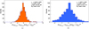 |
Fig. 2. Distribution of the normalized difference between the flux at 20 GeV from the 3FGL and 3FHL catalogs before (panel a) and after (panel b) the correction (see text for details). A Gaussian function has been fit to both histograms; the mean of the distributions, μ, quantifies the mismatch between the fluxes reported in the two catalogs. |
To determine the offset between the fluxes at 20 GeV and the ensuing overall scaling factor to apply to the 3FGL spectral points, the following approach was adopted: (i) the mean of the distribution and its associated error computed through a Gaussian fit – including all the sources – was calculated; (ii) sources that show a deviation from the mean larger than 3σ were excluded; (iii) the quantity r = log(Φ3FHL/Φ3FGL) was calculated, and the 3FGL spectral points were corrected for a factor er; (iv) the procedure from point (i) was repeated until no more outliers were found. The procedure converged at the first iteration, and the final scaling factor, r, is −0.10 ± 0.03, which corresponds to a scaling in flux of 0.90 ± 0.03. Among the whole sample, nine sources were identified as outliers and removed from the sample: 3FHL J0510.0+1800 (PKS 0507+17), 3FHL J0958.7+6533 (QSO B0954+65), 3FHL J1104.4+3812 (Mrk 421), 3FHL J1230.2+2517 (ON 246), 3FHL J1415.6+4830, 3FHL J1427.9−4206 (PKS 1424−418), 3FHL J1443.9+2502 (PKS 1441+25), 3FHL J1522.6−2731, and 3FHL J1728.3+5013 (QSO B1727+502).
A possible explanation concerning the flux mismatch between the two catalogs lies in the high variability of the sources: strong flares can contribute to slightly modify the average flux level over two different time-spans. In order to investigate this hypothesis, the distribution of the 3FGL variability index was inspected. Six out of nine sources show a variability index above a threshold of 72.44 (indicating a probability of 1% of being a steady source): 3FHL J0510.0+1800 (114.8), 3FHL J0958.7+6533 (210.7), 3FHL J1104.4+3812 (755.1), 3FHL J1230.2+2517 (95.3), 3FHL J1427.9−4206 (3146.8), and 3FHL J1522.6−2731 (182.9). The three remaining outliers are characterized by a variability index below the threshold: 3FHL J1415.6+4830 (53.9), 3FHL J1443.9+2502 (48.0), and 3FHL J1728.3+5013 (54.1). This indicates that variability may play a role, but it might not be the only factor responsible for the flux mismatch.
Figure 2b shows the distribution obtained after correction for a scaling factor r = −0.10. The distribution is well centered on zero, but shows a spread slightly smaller than one. This small discrepancy with a standard normal distribution is expected since we are dealing with nonindependent datasets containing double counting of data from catalogs characterized by different statistics.
To investigate the effect of the variability, we split the sample (including the nine outlier sources mentioned above) into steady and variable sources, according to the estimators from both the 3FGL and the 3FHL catalogs. In particular, we classified as steady sources those characterized by a variability index (3FGL) <71.5 and a number of Bayesian blocks (3FHL) = 1. This cut results in two subsamples, steady and variable, containing 249 and 250 sources, with associated scaling factors of −0.02 ± 0.03 and −0.22 ± 0.03, respectively. Such a difference could derive from the fact that the 3FHL catalog contains 3 years more data than the 3FGL. Since steady sources should not show detectable variability, no measurable change is expected in their flux over long periods. Variable sources on the contrary might have shown variability over the three extra years covered by the 3FHL. Furthermore, we note that 3FHL data have been processed with the event-level analysis Pass8, while Pass7 was used for the 3FGL. Given that no firm conclusion can be drawn as to the origin of the discrepant scaling factor, we use r = −0.1 ± 0.1 and treat the uncertainty as a systematic effect (see Sect. 5).
To summarize, starting from a list of 509 sources, 13 were excluded because of an incorrect or unreliable redshift, 3 sources were added that have a solid redshift measurement and at least one significant point in the 3FHL spectrum, and 9 outlying sources with a large difference between the 3FGL and 3FHL flux were also excluded. The final sample contains 490 sources with a redshift between 0.003 and 2.534. To be conservative, the first point of the 3FGL catalog (at 173 MeV) was excluded from the analysis because of the low Fermi-LAT acceptance2. Both catalogs report the flux measured at 31.6 GeV. The 3FHL point at 31.6 GeV was included in the fit because of a much larger statistic. Finally, the upper limits (ULs) were not considered in the fitting procedure due to the lack of a robust way of treating them.
4. Analysis method
4.1. Extragalactic background light absorption
The process responsible for the γ-ray opacity is the electron–positron pair production that occurs when γ-rays interact with photons of the EBL.
The effect of the γ-ray attenuation is encoded in the EBL optical depth:
![Mathematical equation: $$ \begin{aligned} \tau {(E_0, z_0)} =&\int ^{z_0}_0 \mathrm{d}z \frac{\partial L}{\partial z}(z) \int ^{\infty }_0 \mathrm{d}\epsilon \frac{\partial n}{\partial \epsilon }(\epsilon , z)\nonumber \\&\times \int ^{-1}_1 \mathrm{d}\cos \theta \frac{1- \cos \theta }{2} \sigma _{\gamma \gamma } E_0(1+z), \epsilon ,\cos \theta )], \end{aligned} $$](/articles/aa/full_html/2019/07/aa34240-18/aa34240-18-eq4.gif) (1)
(1)
that is given by multiplying the number density of the background photon field, n, with the process cross section, σγγ, and then by integrating over the distance, the scattering angle, and the energy of the background photons in the comoving frame. The cross-section reaches its maximum when the energy of EBL photons is ∼1 eV × (E/500 GeV)−1, which means that high-energy γ-rays mostly interact with COB photons, while VHE photons interact with CIB ones. Finally, ultra-high-energy photons (UHE > 1 PeV) interact mainly with photons of the CMB.
The effect of the EBL on γ-ray emission of blazars leaves an imprint on their spectra. In particular, the spectrum is attenuated by a factor:
 (2)
(2)
where Φobs and Φintr are the observed and intrinsic spectrum, respectively, and τ(E0, z0) is the EBL optical depth. The total amount of absorption depends on the energy of the γ-ray, the source distance, and the density of the EBL photon field. Since direct measurements of the EBL are not easy to obtain for the reasons explained in Sect. 1, many EBL models have been built to estimate the EBL optical depth as a function of redshift, and to derive the ensuing absorption in spectra of high-energy sources.
In this paper, we use the EBL models of Franceschini et al. (2008; FR08 hereafter), Domínguez et al. (2011; DOM11), Gilmore et al. (2012; GIL12), and Franceschini & Rodighiero (2017, 2018; FR17).
4.2. Likelihood analysis
An EBL scaling factor, α, is introduced (e.g., Ackermann et al. 2012; H.E.S.S. Collaboration 2013; Biteau & Williams 2015), and Eq. (2) can be rewritten as:
 (3)
(3)
where the parameter α indicates the agreement between a given EBL model and the γ-ray observations: α = 0 corresponds to the absence of absorption, while α = 1 implies that the model predictions are in perfect agreement with the γ-ray data. The main goal of this work is to derive the scaling factor for different state-of-the-art EBL models as a function of redshift to test the model predictions against γ-ray data. By combining several blazar spectra, it is possible to derive the mean deviation between the observed and the intrinsic spectra, and hence the EBL optical depth, τ(E0, z0).
We performed a joint fit of the EBL scaling factor, α, and of the intrinsic spectral parameters of all the sources. The fitting procedure consists in four main steps: (i) A common functional form, one of four different spectral shapes given in Eqs. (4)–(7), is chosen to model the intrinsic spectrum, Φintr, of all the sources. (ii) For α from 0 to 3 (with step of 0.02), the best-fit spectral parameters of each source are determined, together with the best α according to the cumulative χ2 of the set of individual fits. (iii) Alternative γ-ray spectral models are considered for each source, fixing α to its best value obtained in (ii). All of the other possible models that have at least one degree of freedom in the spectral fit are tested for each source. If another model is preferred by at least 2σ (see arguments in the following section), it is chosen as the new model for that source. If more than one model is preferred, the simplest model (in the case of a different number of degrees of freedom) or the most preferred one (in case of the same number of degrees of freedom) is selected. This iterative selection (ii–iii) keeps going on until the convergence on the model set is reached. This prevents the results from being biased by an inappropriate choice of intrinsic γ-ray spectral models. (iv) Finally, the likelihood profile is computed as a function of α in order to find the statistical uncertainty associated with the best scaling factor. The full fitting procedure is illustrated in the diagram of Fig. 3.
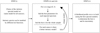 |
Fig. 3. Diagram illustrating the steps of the fitting procedure. |
4.3. γ-ray spectral model selection
Equation (2) points out that an accurate estimate of the EBL depends crucially on the assumptions on the intrinsic spectral shape, especially if we consider that the emission processes of blazars are still not fully understood. In other words, it may seem difficult at first to disentangle intrinsic curvature from interaction with EBL photons.
In order to avoid bias in the results due to an inappropriate choice of intrinsic spectral models, various functions have been tested for each source: power law (PWL, hereafter)
 (4)
(4)
exponential cutoff power law (EPWL),
 (5)
(5)
log-parabola (LP),
 (6)
(6)
and exponential cutoff log-parabola (ELP),
 (7)
(7)
where Φ0 is the flux normalization, E0 is a reference energy (set as  , where Emin and Emax are the minimum and the maximum energy of the Fermi-LAT spectrum, respectively), a is the spectral index, b is the curvature parameter, and Ecut is the energy corresponding to the cutoff energy.
The best spectral model for each source is computed iteratively in a procedure explained in Sect. 4.2. Since the approach we follow is not based on a specific assumption on the intrinsic spectral models, a criterion to discriminate among different models is needed. The switch occurs if a model is preferred at a certain σ level with respect to another one3:
![Mathematical equation: $$ \begin{aligned} \sigma = \sqrt{2} \, \text{ erfc}^{-1} \left[ P(\Delta \chi ^2, \Delta \text{ d.o.f.}) \right], \end{aligned} $$](/articles/aa/full_html/2019/07/aa34240-18/aa34240-18-eq12.gif) (8)
(8)
where erfc−1 is the inverse complementary error function, Δχ2 is the difference in the χ2 obtained for the two comparing models, and Δdof is the difference of the number of parameters of the two models. We note that the PWL–LP–ELP and PWL–EPWL–ELP models presented above are nested, enabling a straightforward estimation of the significance. In cases where a choice between an LP and EPWL model is needed, the model with the largest significance with respect to a PWL is chosen.
To determine the best σ threshold, we checked the compatibility between the observed χ2-probability distribution over the sample of sources and a uniform distribution through a Kolmogorov–Smirnov (KS) test (an example is shown in Fig. 4). For several σ values in the range 1 ≤ σ ≤ 3, the KS probability of obtaining a deviation, D, between the observed and ideal distribution of the χ2 probability distribution of the individual spectra, that is larger than the observed one (in case the null hypothesis is true, i.e., the two distributions are the same) has been calculated as (Press et al. 2007):
![Mathematical equation: $$ \begin{aligned} P(D < \mathrm{observed}) = P_{\rm KS} \left[ \left( \sqrt{N_{\rm e}} + 0.12 +\frac{0.11}{\sqrt{N_{\rm e}}} \right) D \right], \end{aligned} $$](/articles/aa/full_html/2019/07/aa34240-18/aa34240-18-eq13.gif) (9)
(9)
where the CDF, PKS(z) (defined for positive z), is defined by the series:
 (10)
(10)
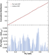 |
Fig. 4. Example of the Kolmogorov–Smirnov statistic obtained for the whole sample, by injecting LP functions as intrinsic spectral models and for σ = 2 (see text for details). Top panel: comparison between the CDF of the χ2 probabilities resulting from the fit and the CDF of a uniform distribution. Bottom panel: bar chart of the distance between the two CDFs as a function of each measured χ2 probability. |
The results obtained starting from different sets of initial spectral models are reported in Fig. 5. Although the initialization is done with different spectral models, the final selected ones can end up being the same (i.e. coincident points in Fig. 5), and this comes in favor of the robustness of the model selection. For low (e.g., 1σ) and high σ values (e.g., 3σ), the KS probability is low, which means that the χ2-probability distribution is far from being compatible with a uniform distribution, which is the distribution expected in case of a healthy fit procedure. Conversely, higher values of the KS probability indicate a compatibility between the χ2 probability and a uniform distribution4.
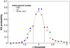 |
Fig. 5. Kolmogorov–Smirnov probability as a function of the σ threshold used to switch to a more complex intrinsic spectral model (results obtained starting from EPWL and ELP models are coincident). The results were obtained by using the EBL model of Gilmore et al. (2012) and different starting spectral models, as discussed in Sect. 4.2. Dotted vertical lines at 1.8 and 2.2 correspond to σ values used to estimate the systematic uncertainties due to the model selection (see text for details). |
A Gaussian was fitted to each set between 1.4 and 2.6, and all of them lead to a mean σ threshold of 2.0 and a standard deviation of 0.2. Therefore, the adopted threshold for the model selection is σ = 2.0 (corresponding to the highest KS probability), and the standard deviation is used to estimate the systematic uncertainty related to the model selection.
5. Results
The EBL scaling factor was obtained for four different EBL models: FR08, DOM11, GIL12, and FR17. Each spectrum considered in the fit includes points retrieved from both the 3FGL and the 3FHL Fermi-LAT catalogs, whose treatment is explained in Sect. 3. The final α values reported in Table 1 correspond to the average among those obtained starting from different initial spectral models:
 (11)
(11)
and the related statistical uncertainties are estimated by:
 (12)
(12)
where σPWL, σLP, σEPWL, and σELP are estimated from the likelihood profile, and correspond to a drop of 1/e from the maximum.
EBL scaling factors α and related uncertainties obtained for different EBL models.
Two subsamples were analyzed depending on the object class: BL Lacs and FSRQs. The FSRQ sample contains 157 objects in the redshift range 0.097 ≤ z ≤ 2.534, while the BL Lac sample contains 299 objects with a redshift 0.032 ≤ z ≤ 2.471. The other 34 sources include 8 radio galaxies, 24 sources marked as unknown, a narrow-line Seyfert I, and a starburst galaxy. Figure 6 reports the results obtained for the whole sample, the BL Lac sample, and the FSRQ sample, respectively. Results include both statistical and systematic uncertainties; the estimation of the latter is described below.
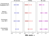 |
Fig. 6. EBL scaling factor obtained analyzing the whole sample (left), FSRQs (center), and BL Lacs (right) for FR17, GIL12, DOM11, and FR17 EBL models. Light colors report the statistical uncertainties, while dark colors include also the systematic ones. |
The source sample has also been divided into four redshift bins of similar size: (i) z ≤ 0.21 containing 123 sources; (ii) 0.21 ≤ z < 0.456 containing 123 sources; (iii) 0.456 ≤ z < 0.944 containing 123 sources, and (iv) 0.944 ≤ z ≤ 2.534 containing 121 sources. Results are reported in Fig. 7.
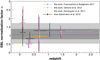 |
Fig. 7. EBL scaling factor obtained for different redshift bins for FR17, GIL12, and DOM11 EBL models. Light colors refer to the statistical uncertainties, while darker colors include also the systematic ones. Comparison with (Ackermann et al. 2012) is also shown (gray). The shaded regions show the 1σ (dark gray) and 2σ (light gray) confidence intervals obtained for the whole sample, using the GIL12 EBL model and including both statistical and systematic uncertainties. |
The approach described in this paper is affected by two kinds of systematic errors: (i) the choice of the σ-threshold (used to switch among the intrinsic spectral models; see Sect. 4.3), and (ii) the injected spectral models which act as a seed for the model-selection procedure. The first is estimated on the whole sample using LP functions as starting γ-ray spectral models, the GIL12 EBL model, and varying the σ-threshold from its optimal value (σ = 2) by an amount equal to the standard deviation obtained from the fit of the KS probability (see Sect. 4.3):
![Mathematical equation: $$ \begin{aligned} \sigma _{\rm syst_{\sigma -thr}}&= \sqrt{\frac{[\alpha _{(2\sigma ,\mathrm{LP})} - \alpha _{(1.8\sigma ,\mathrm{LP})}]^2 + [\alpha _{(2\sigma ,\mathrm{LP})} - \alpha _{(2.2\sigma ,\mathrm{LP})}]^2}{2}} \nonumber \\&= 0.16. \end{aligned} $$](/articles/aa/full_html/2019/07/aa34240-18/aa34240-18-eq45.gif) (13)
(13)
The resulting 0.16 is used as a contribution to the systematic uncertainty for all values of α. The choice of injecting a LP function to model the intrinsic spectra does not have a significant impact on the estimation of this uncertainty.
The second source of systematic uncertainty is estimated by fixing the σ threshold to its optimal value, and by varying the starting spectral models:
![Mathematical equation: $$ \begin{aligned} \sigma _{\rm syst_{mod.sel.}} = &\left[[ (\alpha _{(\sigma =2.0, \mathrm{PWL})} - \alpha )^2 + (\alpha _{(\sigma =2.0, \mathrm{LP})} - \alpha )^2 \right. \nonumber \\& \left. + (\alpha _{(\sigma =2.0, \mathrm{EPWL})} - \alpha )^2 + (\alpha _{(\sigma =2.0, \mathrm{ELP})} - \alpha )^2 ]/4 \right] ^{1/2}. \end{aligned} $$](/articles/aa/full_html/2019/07/aa34240-18/aa34240-18-eq46.gif) (14)
(14)
A source of systematic uncertainty specific to this study is related to the flux scaling factor applied to the 3FGL spectral points (see Sect. 3.2). The two different scaling factors obtained for the steady and the variable samples were applied to all the sources studied in this work. The systematic uncertainty σsystflux−;corr. is estimated as the difference between the EBL normalization obtained with the whole-sample scaling factor, and those obtained with the steady- and variable- sample scaling factors.
Contrary to the σ threshold, the uncertainties related to the injected models and flux scaling factor are estimated for each bin, since they may have a different impact depending on the redshift (i.e., on the absorption amount due to the EBL photons). For reference, we obtain σsystmod.sel. = 0.01 and σsystflux−;corr. = −0.18 + 0.28 with the model of GIL12 applied to the full sample.
Finally, statistic and systematic uncertainties were added in quadrature to obtain the total error:
 (15)
(15)
6. Discussion
A sample of 490 blazars observed with Fermi-LAT was used to determine the EBL normalization, α, for the EBL models of FR08, DOM11, GIL12, and FR17. The joint fit of the EBL optical depth and of the intrinsic spectra of the sources was performed allowing any of four possible intrinsic γ-ray spectral shapes. A set of intrinsic spectral models is injected at the beginning of the fitting procedure, and the choice for each source is left free to vary according to the best overall fit to the data. The systematic uncertainties induced by the choice of the initial intrinsic models were estimated for the injected models and the selection criterion. Another source of systematic uncertainty derives from the flux scaling factor applied to correct the offset between the two catalogs. An important role in the determination of such a factor might be played by the source variability or by the low statistics at higher energies. This systematic uncertainty, specific to this study and not intrinsic to the method itself, is comparable to and often larger than the others.
The analysis performed on the whole sample gives an EBL normalization, α, ranging from 1.04 to 1.13, which is compatible with a value of 1 for all the EBL models, with a typical statistical uncertainty of ∼10–12%, and a total uncertainty (statistical + systematic) of ∼25–34%, and up to 39% for the DOM11 EBL-model.
Sources were divided into BL Lacs and FSRQs in order to see if internal absorption plays a different role in different object types, possibly biasing the EBL estimation. The values of the scaling factor, α, obtained for the two subsamples are perfectly compatible with each other, but the analysis ends up with a significant difference in the final intrinsic γ-ray spectral models. The intrinsic spectra of BL Lacs are modeled mainly by PWL, ∼80%, and by only ∼16% of LP and EPWL. The latter percentage rises to ∼45% in the case of FSRQs, which are modeled by a PWL in only ∼55% of sources. An explanation for this can be found in the fact that FSRQs are characterized by a synchrotron peak located at low energies (νs < 1014.5 Hz), while the peak distribution of BL Lacs is shifted to higher energies by at least one order of magnitude (Giommi et al. 2012). The high-energy component of blazar spectra similarly exhibit a maximum in their SED located at energies >1 TeV and ≤100 GeV for BL Lacs and FSRQs, respectively. Therefore, the difference in the percentage of intrinsic models of a particular type can be explained by the energy range explored by Fermi-LAT.
The sample was then split into four redshift bins, each containing a similar number of sources. Within each bin, similar values of the EBL scaling factor were found for the four EBL models. All results are compatible within 2σ with the EBL normalization obtained for the whole sample.
Finally, from Table 1, we note that the percentage of sources preferring PWL and LP changes slightly as the redshift increases. In particular, moving to higher redshift the fraction of PWL models decreases (from ∼85 to ∼63%), while the fraction of LP models increases (from ∼8 to ∼24%), and similarly for EPWL (from ∼6 to ∼15%). The evolution of the fraction of LP models can be understood from the presence of a larger number of FSRQs at higher redshift, with FSRQs peaking at lower energies than BL Lacs.
In Fig. 8, the EBL normalizations obtained in this work are compared with those present in the literature. In the top panel of Fig. 8, our results obtained with FR17 are compared to existing results obtained with FR08. We note that in FR17, most of the updates in the EBL spectrum with respect to FR08 have modified the CIB peak in the mid- to far-infrared ranges. Since the COB peak provides the EBL photons interacting with γ-rays detectable by Fermi-LAT, we expect that changes in FR17 only slightly affect the results obtained using the Fermi-LAT data, and hence that the results are comparable to those obtained by adopting the FR08 EBL model. The difference between the results obtained with the two models is ∼6% for the first and the second bin, ∼10% for the third bin, ∼8% for the fourth bin, and ∼8% for the whole sample.
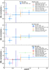 |
Fig. 8. Comparison among the results in the literature and those obtained in this work. Comparisons are shown for different EBL models: FR08 and FR17 (top), GIL12 (central), and DOM11 (bottom). |
The results of this work obtained for the first two bins – adopting the FR17 EBL model – are compatible with those obtained for FR08 in Ackermann et al. (2012), where a smaller sample of 150 blazars was analyzed assuming an intrinsic spectral shape described by an LP function. The results presented here are also consistent with the results of H.E.S.S. Collaboration (2013) and of Mazin et al. (2017).
Compatible results with this work are seen from the comparison of the EBL scaling factor obtained from the individual blazar PKS 1441+25 (Ahnen et al. 2015) and the lensed blazar B2 018+357 (Ahnen et al. 2016a).
From Fig. 8, one could possibly infer a tension between the results of this work and those (i) in Ahnen et al. (2016b) obtained around z ∼ 0.2, in Biteau & Williams (2015) obtained with TeV sources in the redshift range 0.019 < z < 0.287, and in Acciari et al. (2019) obtained with GeV–TeV sources in the redshift range 0.14 ≤ z ≤ 0.212; and (ii) in Armstrong et al. (2017), obtained with 17 GeV sources in the redshift range 0.847 < z < 1.596. In order to investigate if a discrepancy is effectively present, we performed a dedicated analysis in the same redshift ranges as those used in the literature. Results obtained at low redshifts (0.019 ≤ z ≤ 0.287) are compatible with those shown in Biteau & Williams (2015), differing by 0.2σ for the FR08 EBL model, 0.6σ for GIL12, and 0.5σ for DOM11. Results obtained in the redshift range 0.14 ≤ z ≤ 0.212 for the DOM11 EBL model show a 2.3σ tension with respect to those obtained in Acciari et al. (2019). At higher redshifts (0.85 ≤ z ≤ 1.596), the comparison with results in Armstrong et al. (2017) shows a small tension: 1.7σ for the FR08 EBL model, and 1.6σ for DOM11. On the contrary, the result of these latter authors for the GIL12 EBL model is in agreement with that presented in this work (0.8σ), as well as results presented in Ahnen et al. (2015) and Ahnen et al. (2016a).
Recently, Abdollahi et al. (2018) carried out studies on the EBL using a large sample of 739 AGNs detected with the Fermi-LAT telescope. These latter authors obtained normalization factors (with 1σ confidence range) of 1.30 ± 0.10, 1.31 ± 0.10, and 1.25 ± 0.10 for the GIL12, DOM11, and FR17 EBL model, respectively. These values are compatible with those obtained in this work for the whole sample, considering both statistical and systematic uncertainties.
7. Conclusion
This paper exams a methodology to determine the scaling factor for different EBL models, avoiding a priori assumptions on the intrinsic spectra of the sources as much as possible. In fact, the spectral curvature is a critical factor that might affect a reliable estimation of the EBL scaling factor, whose impact may not have been fully quantified thus far since the internal emission and the absorption processes at play in blazars are not fully understood. Not accounting for curvature can lead to an overestimation of the scaling factor, attributing all the absorption to the EBL. On the contrary, an intrinsic curvature that is too accentuated can retrace the EBL absorption, leading to an underestimation of the latter. The approach we use, expanding on that presented in Biteau & Williams (2015), leaves the intrinsic spectral models free in the fitting procedure, avoiding a fixed intrinsic γ-ray spectral shape. This approach is accompanied by a careful study of the systematic uncertainties, possibly the first of its kind, where four different functions are used as candidates to model the intrinsic spectra.
The EBL scaling factors obtained by analyzing 490 Fermi-LAT archival spectra with this method are in good agreement with those presented in the literature, and they were obtained with a robust approach. In this work, the study of the evolution of the EBL appears to be limited by the systematic uncertainties due to model selection. An interesting comparison would consist of applying the approach described in this paper to the larger sample of Abdollahi et al. (2018), who adopted another method to find the EBL normalization, and to run a dedicated spectral analysis exploiting the full potential of Fermi-LAT data rather than using archival catalog data. Moreover, constraints on the EBL evolution can potentially be improved using the Fermi-LAT Fourth Source Catalog (4FGL)5, or more specifically the 4LAC, which will feature spectral points and redshifts of AGNs. This will allow the unabsorbed part of the spectrum to be better constrained. Finally, the future Cherenkov Telescope Array (CTA) ground-based γ-ray observatory (CTA Consortium 2019), with its unprecedented sensitivity, will be a crucial instrument for a better understanding of the EBL.
In the selection process the priority is given to simpler models, i.e., simpler models are compared to more and more complex ones.
We investigated the presence of outliers at a χ2 probability close to zero and one. We find three spectra with a χ2 probability lower than 0.1%, which is expected with a probability of 0.1% for a sample of 490 objects. We verified that excluding these three sources from the analysis does not impact our results. Similar conclusions are drawn for each of the subsamples studied in this paper.
Acknowledgments
We are grateful for a fruitful exchange with the anonymous referee, which helped to improve the quality of this paper. We thank Paolo Goldoni for feedback on the redshifts of the sources studied in this work. We acknowledge support from the U.S. NASA Fermi-GI Cycle 9 grant NNX16AR40G. This work was also supported by the Programme National Hautes Energies with the founding from CNRS (INSU/ INP3/INP), CEA, and CNES. Moreover, we thank U.S. National Science Foundation for support under grants PHY-1307311 and PHY-1707432 as well as P2IO LabEx (ANR-10-LABX-0038) in the framework “Investissements d’Avenir” (ANR-11-IDEX-0003-01) managed by the “Agence Nationale de la Recherche” (ANR, France).
References
- Abdollahi, S., Ackermann, M., Ajello, M., et al. 2018, Science, 362, 1031 [NASA ADS] [CrossRef] [Google Scholar]
- Abeysekara, A. U., Archambault, S., Archer, A., et al. 2015, ApJ, 815, L22 [NASA ADS] [CrossRef] [Google Scholar]
- Abolfathi, B., Aguado, D. S., Aguilar, G., et al. 2018, ApJS, 235, 42 [NASA ADS] [CrossRef] [Google Scholar]
- Acciari, V. A., Ansoldi, S., Antonelli, L. A., et al. 2019, MNRAS, 486, 4233 [NASA ADS] [CrossRef] [Google Scholar]
- Acero, F., Ackermann, M., Ajello, M., et al. 2015, ApJS, 218, 23 [Google Scholar]
- Ackermann, M., Ajello, M., Allafort, A., et al. 2012, Science, 338, 1190 [NASA ADS] [CrossRef] [Google Scholar]
- Ackermann, M., Ajello, M., Allafort, A., et al. 2013, ApJS, 209, 34 [NASA ADS] [CrossRef] [Google Scholar]
- Ackermann, M., Ajello, M., Atwood, W. B., et al. 2015, ApJ, 810, 14 [NASA ADS] [CrossRef] [Google Scholar]
- Aharonian, F. A. 2000, New A, 5, 377 [NASA ADS] [CrossRef] [Google Scholar]
- Ahnen, M. L., Ansoldi, S., Antonelli, L. A., et al. 2015, ApJ, 815, L23 [NASA ADS] [CrossRef] [Google Scholar]
- Ahnen, M. L., Ansoldi, S., Antonelli, L. A., et al. 2016a, A&A, 595, A98 [NASA ADS] [CrossRef] [EDP Sciences] [Google Scholar]
- Ahnen, M. L., Ansoldi, S., Antonelli, L. A., et al. 2016b, A&A, 590, A24 [NASA ADS] [CrossRef] [EDP Sciences] [Google Scholar]
- Ajello, M., Atwood, W. B., Baldini, L., et al. 2017, ApJS, 232, 18 [NASA ADS] [CrossRef] [Google Scholar]
- Armstrong, T., Brown, A. M., & Chadwick, P. M. 2017, MNRAS, 470, 4089 [NASA ADS] [CrossRef] [Google Scholar]
- Atwood, W. B., Baldini, L., Bregeon, J., et al. 2013, ApJ, 774, 76 [NASA ADS] [CrossRef] [Google Scholar]
- Band, D. L., & Grindlay, J. E. 1985, ApJ, 298, 128 [NASA ADS] [CrossRef] [Google Scholar]
- Biteau, J., & Williams, D. A. 2015, ApJ, 812, 60 [NASA ADS] [CrossRef] [Google Scholar]
- Bregeon, J., Charles, E., & Wood, M., for the Fermi-LAT collaboration 2013, ArXiv e-prints [arXiv:1304.5456] [Google Scholar]
- CTA Consortium 2019, Science with the Cherenkov Telescope Array (World Scientific Publishing Co) [Google Scholar]
- Desai, A., Ajello, M., Omodei, N., et al. 2017, ApJ, 850, 73 [NASA ADS] [CrossRef] [Google Scholar]
- Dole, H., Lagache, G., Puget, J.-L., et al. 2006, A&A, 451, 417 [NASA ADS] [CrossRef] [EDP Sciences] [MathSciNet] [Google Scholar]
- Domínguez, A., Primack, J. R., Rosario, D. J., et al. 2011, MNRAS, 410, 2556 [NASA ADS] [CrossRef] [Google Scholar]
- Driver, S. P., Andrews, S. K., Davies, L. J., et al. 2016, ApJ, 827, 108 [NASA ADS] [CrossRef] [Google Scholar]
- Dwek, E., & Arendt, R. G. 1998, ApJ, 508, L9 [NASA ADS] [CrossRef] [Google Scholar]
- Dwek, E., & Krennrich, F. 2013, Astropart. Phys., 43, 112 [NASA ADS] [CrossRef] [Google Scholar]
- Finke, J. D., & Razzaque, S. 2009, ApJ, 698, 1761 [NASA ADS] [CrossRef] [Google Scholar]
- Finke, J. D., Razzaque, S., & Dermer, C. D. 2010, ApJ, 712, 238 [NASA ADS] [CrossRef] [Google Scholar]
- Franceschini, A., & Rodighiero, G. 2017, A&A, 603, A34 [NASA ADS] [CrossRef] [EDP Sciences] [Google Scholar]
- Franceschini, A., & Rodighiero, G. 2018, A&A, 614, C1 [CrossRef] [EDP Sciences] [Google Scholar]
- Franceschini, A., Rodighiero, G., & Vaccari, M. 2008, A&A, 487, 837 [NASA ADS] [CrossRef] [EDP Sciences] [Google Scholar]
- Gilmore, R. C., Somerville, R. S., Primack, J. R., & Domínguez, A. 2012, MNRAS, 422, 3189 [NASA ADS] [CrossRef] [Google Scholar]
- Giommi, P., Polenta, G., Lähteenmäki, A., et al. 2012, A&A, 541, A160 [NASA ADS] [CrossRef] [EDP Sciences] [Google Scholar]
- Giovannini, G., Falomo, R., Scarpa, R., Treves, A., & Urry, C. M. 2004, ApJ, 613, 747 [NASA ADS] [CrossRef] [Google Scholar]
- Goldoni, P., Pita, S., Boisson, C., et al. 2016, A&A, 586, L2 [NASA ADS] [CrossRef] [EDP Sciences] [Google Scholar]
- Gould, R. J., & Schréder, G. P. 1967, Phys. Rev., 155, 1408 [NASA ADS] [CrossRef] [Google Scholar]
- Halpern, J. P., Eracleous, M., & Forster, K. 1997, AJ, 114, 1736 [NASA ADS] [CrossRef] [Google Scholar]
- Hauser, M. G., & Dwek, E. 2001, ARA&A, 39, 249 [NASA ADS] [CrossRef] [Google Scholar]
- H.E.S.S. Collaboration (Abramowski, A., et al.) 2013, A&A, 550, A4 [NASA ADS] [CrossRef] [EDP Sciences] [Google Scholar]
- H.E.S.S. Collaboration (Abdalla, H., et al.) 2017, A&A, 606, A59 [NASA ADS] [CrossRef] [EDP Sciences] [Google Scholar]
- Jones, D. H., Read, M. A., Saunders, W., et al. 2009, MNRAS, 399, 683 [NASA ADS] [CrossRef] [Google Scholar]
- Levenson, L. R., & Wright, E. L. 2008, ApJ, 683, 585 [NASA ADS] [CrossRef] [Google Scholar]
- Madau, P., & Pozzetti, L. 2000, MNRAS, 312, L9 [NASA ADS] [CrossRef] [Google Scholar]
- Mannheim, K. 1993, A&A, 269, 67 [NASA ADS] [Google Scholar]
- Mao, L. S. 2011, New Astron., 16, 503 [NASA ADS] [CrossRef] [Google Scholar]
- Mazin, D., & Raue, M. 2007, A&A, 471, 439 [NASA ADS] [CrossRef] [EDP Sciences] [Google Scholar]
- Mazin, D., Domínguez, A., Fallah Ramazani, V., et al. 2017, in 6th International Symposium on High Energy Gamma-Ray Astronomy, AIP Conf. Ser., 1792, 050037 [Google Scholar]
- Meisner, A. M., & Romani, R. W. 2010, ApJ, 712, 14 [NASA ADS] [CrossRef] [Google Scholar]
- Meyer, M., Raue, M., Mazin, D., & Horns, D. 2012, A&A, 542, A59 [NASA ADS] [CrossRef] [EDP Sciences] [Google Scholar]
- Nikishov, A. I. 1962, Sov. Phys. JETP, 14, 393 [Google Scholar]
- Paiano, S., Landoni, M., Falomo, R., et al. 2017, ApJ, 837, 144 [NASA ADS] [CrossRef] [Google Scholar]
- Pita, S., Goldoni, P., Boisson, C., et al. 2014, A&A, 565, A12 [NASA ADS] [CrossRef] [EDP Sciences] [Google Scholar]
- Press, W. H., Teukolsky, S. A., Vetterling, W. T., & Flannery, B. P. 2007, Numerical Recipes 3rd Edition: The Art of Scientific Computing, 3rd edn. (Cambridge University Press) [Google Scholar]
- Razzaque, S., Dermer, C. D., & Finke, J. D. 2009, ApJ, 697, 483 [NASA ADS] [CrossRef] [Google Scholar]
- Rector, T. A., Gabuzda, D. C., & Stocke, J. T. 2003, AJ, 125, 1060 [NASA ADS] [CrossRef] [Google Scholar]
- Shaw, M. S., Romani, R. W., Cotter, G., et al. 2013, ApJ, 764, 135 [NASA ADS] [CrossRef] [Google Scholar]
- Sikora, M., Moderski, R., & Madejski, G. M. 2008, ApJ, 675, 71 [NASA ADS] [CrossRef] [Google Scholar]
- Sinha, A., Sahayanathan, S., Misra, R., Godambe, S., & Acharya, B. S. 2014, ApJ, 795, 91 [NASA ADS] [CrossRef] [Google Scholar]
- Stecker, F. W., & Scully, S. T. 2006, ApJ, 652, L9 [NASA ADS] [CrossRef] [Google Scholar]
- Stecker, F. W., de Jager, O. C., & Salamon, M. H. 1992, ApJ, 390, L49 [NASA ADS] [CrossRef] [Google Scholar]
- Tavecchio, F., Maraschi, L., & Ghisellini, G. 1998, ApJ, 509, 608 [NASA ADS] [CrossRef] [Google Scholar]
All Tables
EBL scaling factors α and related uncertainties obtained for different EBL models.
All Figures
|
Fig. 1. Left panels: 3FHL J2253.9+1608 spectrum, including points from the 3FGL catalog (red), and from 3FHL catalog (blue); upper limits (not included in the fit) are shown in gray. The spectral fit is displayed for the best EBL normalization over the range of interest, and has been performed modeling the intrinsic spectrum with a power law (a), an exponential cutoff power law (b), a log-parabola (c), and an exponential cutoff log-parabola (d). Right panels: likelihood profile as a function of the EBL normalization, α. |
| In the text | |
|
Fig. 2. Distribution of the normalized difference between the flux at 20 GeV from the 3FGL and 3FHL catalogs before (panel a) and after (panel b) the correction (see text for details). A Gaussian function has been fit to both histograms; the mean of the distributions, μ, quantifies the mismatch between the fluxes reported in the two catalogs. |
| In the text | |
|
Fig. 3. Diagram illustrating the steps of the fitting procedure. |
| In the text | |
|
Fig. 4. Example of the Kolmogorov–Smirnov statistic obtained for the whole sample, by injecting LP functions as intrinsic spectral models and for σ = 2 (see text for details). Top panel: comparison between the CDF of the χ2 probabilities resulting from the fit and the CDF of a uniform distribution. Bottom panel: bar chart of the distance between the two CDFs as a function of each measured χ2 probability. |
| In the text | |
|
Fig. 5. Kolmogorov–Smirnov probability as a function of the σ threshold used to switch to a more complex intrinsic spectral model (results obtained starting from EPWL and ELP models are coincident). The results were obtained by using the EBL model of Gilmore et al. (2012) and different starting spectral models, as discussed in Sect. 4.2. Dotted vertical lines at 1.8 and 2.2 correspond to σ values used to estimate the systematic uncertainties due to the model selection (see text for details). |
| In the text | |
|
Fig. 6. EBL scaling factor obtained analyzing the whole sample (left), FSRQs (center), and BL Lacs (right) for FR17, GIL12, DOM11, and FR17 EBL models. Light colors report the statistical uncertainties, while dark colors include also the systematic ones. |
| In the text | |
|
Fig. 7. EBL scaling factor obtained for different redshift bins for FR17, GIL12, and DOM11 EBL models. Light colors refer to the statistical uncertainties, while darker colors include also the systematic ones. Comparison with (Ackermann et al. 2012) is also shown (gray). The shaded regions show the 1σ (dark gray) and 2σ (light gray) confidence intervals obtained for the whole sample, using the GIL12 EBL model and including both statistical and systematic uncertainties. |
| In the text | |
|
Fig. 8. Comparison among the results in the literature and those obtained in this work. Comparisons are shown for different EBL models: FR08 and FR17 (top), GIL12 (central), and DOM11 (bottom). |
| In the text | |
Current usage metrics show cumulative count of Article Views (full-text article views including HTML views, PDF and ePub downloads, according to the available data) and Abstracts Views on Vision4Press platform.
Data correspond to usage on the plateform after 2015. The current usage metrics is available 48-96 hours after online publication and is updated daily on week days.
Initial download of the metrics may take a while.