| Issue |
A&A
Volume 590, June 2016
|
|
|---|---|---|
| Article Number | A113 | |
| Number of page(s) | 18 | |
| Section | Stellar structure and evolution | |
| DOI | https://doi.org/10.1051/0004-6361/201527051 | |
| Published online | 25 May 2016 | |
The X-ray light curve of the massive colliding wind Wolf-Rayet + O binary WR 21a⋆
Groupe d’Astrophysique des Hautes Énergies, Institut d’Astrophysique et de Géophysique, Université de LiègeQuartier Agora (B5c), Allée du 6 Août 19c, 4000 Sart Tilman Liège Belgium
e-mail: gosset@astro.ulg.ac.be
Received: 24 July 2015
Accepted: 13 January 2016
Our dedicated XMM-Newton monitoring, as well as archival Chandra and Swift datasets, were used to examine the behaviour of the WN5h+O3V binary WR 21a at high energies. For most of the orbit, the X-ray emission exhibits few variations. However, an increase in strength of the emission is seen before periastron, following a 1 /D relative trend, where D is the separation between both components. This increase is rapidly followed by a decline due to strong absorption as the Wolf-Rayet (WR) comes in front. The fitted local absorption value appears to be coherent with a mass-loss rate of about 1 × 10⁻⁵ M⊙ yr-1 for the WR component. However, absorption is not the only parameter affecting the X-ray emission at periastron as even the hard X-ray emission decreases, suggesting a possible collapse of the colliding wind region near to or onto the photosphere of the companion just before or at periastron. An eclipse may appear as another potential scenario, but it would be in apparent contradiction with several lines of evidence, notably the width of the dip in the X-ray light curve and the absence of variations in the UV light curve. Afterwards, the emission slowly recovers, with a strong hysteresis effect. The observed behaviour is compatible with predictions from general wind-wind collision models although the absorption increase is too shallow.
Key words: stars: early-type / stars: Wolf-Rayet / stars: winds, outflows / X-rays: stars / stars: individual: WR 21a
© ESO, 2016
1. Introduction
Massive stars of type O and early B, and Wolf-Rayet (WR) stars, their evolved descendants, are very important objects that have a large impact on their host galaxy. Indeed, they participate in the chemical evolution of the interstellar medium and dominate the mechanical evolution of their surroundings by carving bubbles and influencing star formation. Despite this importance, the main fundamental physical parameters characterising them remain poorly known and the actual details of massive star evolution are yet to be understood (e.g. the luminous blue variable phase, the effect of rotation and the corresponding internal law). This is particularly true for the most massive objects.
Certainly the main basic parameter is the mass. Classically, astronomers supposed that the most massive stars were to be found amongst very early (O2–O3) stars. However, recent clues tend to prove that the most massive stars evolve rapidly towards core-hydrogen-burning objects appearing as disguised hydrogen-rich WR stars, of the WNLh (late H-rich WN) type. In that context, binary system investigations played a key role in recognising the true nature of WNLh stars. The relatively small number of extremely massive Galactic stars implies that the discovery and in-depth study of any such system provide breakthrough information bringing new constraints on stellar evolution.
The second crucial parameter for massive star evolution is the mass-loss rate, which remains not well known, mainly due to uncertain clumping properties. Therefore, a large palette of possible values are usually obtained for any star. In a massive binary system, the winds of both stars collide in a so-called colliding wind region (CWR) broadly located between the two stars. In some cases, a plasma at high temperature (some 107 K) is generated, which then emits an intense thermal X-ray emission in addition to the intrinsic emission1. The variation of the former emission along the orbital cycle should provide information on the shape of the shock and its hydrodynamical nature. This variation is therefore an important source of knowledge of the relative strengths of the winds, hence, of the respective mass-loss rates. The evolution with phase of the observed emission also varies because of the changing absorbing column along the line of sight which depends on the inclination of the system and the mass-loss rates. Therefore, the X-ray light curves of CWRs are of high diagnostic value for winds of massive stars.
In the above mentioned context, WR 21a is a very interesting object. Known as an X-ray source since Einstein observations, it was the first Wolf-Rayet star discovered thanks to its X-ray emission (Mereghetti & Belloni 1994; Mereghetti et al. 1994). Follow-up optical studies (Niemela et al. 2006, 2008; Tramper et al. 2016) showed that WR 21a is actually a WN5+O3 binary system with a 31.7 d orbit. The suggested mass for the primary WN star is ~100 M⊙, making it one of the few examples of very high-mass stars. In order to deepen our knowledge of WR 21a, we acquired four X-ray observations with the XMM-Newton facility. Our aim was to obtain an X-ray light curve for this supposed colliding-wind system as well as X-ray spectra to interpret the behaviour of the collision zone along the orbital cycle. By adding archival data, we present a first interpretation of the X-ray light curve of this outstanding massive binary system. Sect. 2 contains the description of the observations and of the relevant reduction processes. Section 3 presents detailed information on the system, whilst Sect. 4 yields our analysis of the X-ray data. A discussion of the results is provided in Sect. 5 whilst we summarise and conclude in Sect. 6.
2. Observations and data reduction
2.1. Optical spectroscopy
As a support to the XMM-Newton observations, we acquired a few high resolution spectra of WR 21a with the FEROS spectrograph (Kaufer et al. 1999) linked to the ESO/MPG 2.2 m telescope at the European Southern Observatory at La Silla (Chile). Three spectra were secured in a run in 2006 (ObsID = 076.D-0294, PI E. Gosset) and three in June 2013 (ObsID = 091.D-0622, PI E. Gosset). The latter spectra are of particular importance since they are contemporaneous with the XMM-Newton pointings. A journal of the observations is provided in Table 1.
The FEROS instrument provides 39 orders covering the entire optical wavelength domain, going from 3800 to 9200 Å with a resolving power of 48 000. The detector was a 2k × 4k EEV CCD with a pixel size of 15 μm × 15 μm. For the reduction process, we used an improved version of the FEROS pipeline working under the MIDAS environment (Sana et al. 2006; Mahy et al. 2012). The data normalisation was then performed by fitting polynomials of degree 4−5 to carefully chosen continuum windows. We mainly worked on the individual orders, but the regions around the Si iv λλ4089, 4116, He ii λ4686, and Hα emission lines were normalised on the merged spectrum as these lines appear at the limit between two orders. Despite a one hour exposure time, the spectra have a S/N ratio of about 50−100 at the best, because of the faintness of the target.
Journal of the optical observations.
2.2. X-ray observations
2.2.1. XMM - Newton
WR 21a was observed four times with XMM-Newton between mid-June 2013 and July 2013 (orbits 2475, 2496, 2497 and 2497; see Table A.1) in the framework of the programme 072419 (PI E. Gosset). The X-ray observations were made in the full-frame mode and the medium filter was used to reject optical/UV light. The data were reduced with SAS v13.5.0 using calibration files available in mid-October 2014 and following the recommendations of the XMM-Newton team2. Data were filtered for keeping only best-quality data (pattern of 0–12 for MOS and 0–4 for pn). A background flare affecting the end of the last observation was also cut. A source detection was performed on each EPIC dataset using the task edetect_chain on the 0.4–2.0 (soft), 2.0–10.0 (hard), and 0.4–10.0 keV (total) energy bands and for a log-likelihood of 10. This task searches for sources using a sliding box and determines the final source parameters from point spread function (PSF) fitting; the final count rates correspond to equivalent on-axis, full PSF count rates (Table A.1).
We then extracted EPIC spectra of WR 21a using the task especget in circular regions of 30′′ radius (to avoid nearby sources) centred on the best-fit positions found for each observation. For the background, a circular region of the same size was chosen in a region devoid of sources and as close as possible to the target; its relative position with respect to the target is the same for all observations. Dedicated ARF and RMF response matrices, which are used to calibrate the flux and energy axes, respectively, were also calculated by this task. EPIC spectra were grouped, with specgroup, to obtain an oversampling factor of five and to ensure that a minimum signal-to-noise ratio of 3 (i.e. a minimum of 10 counts) was reached in each spectral bin of the background-corrected spectra.
Light curves of WR 21a were extracted, for time bins of 200 s and 1 ks, in the same regions as the spectra and in the same energy bands as the source detection. They were further processed by the task epiclccorr, which corrects for loss of photons due to vignetting, off-axis angle, or other problems such as bad pixels. In addition, to avoid very large errors and bad estimates of the count rates, we discarded bins displaying effective exposure time lower than 50% of the time bin length. Our previous experience with XMM-Newton has shown us that including such bins degrades the results. As the background is much fainter than the source, in fact too faint to provide a meaningful analysis, three sets of light curves were produced and analysed individually: the raw source+background light curves, the background-corrected light curves of the source and the light curves of the sole background region. The results found for the raw and background-corrected light curves of the source are indistinguishable.
2.2.2. Swift
WR 21a was observed 198 times by Swift in October− November 2013, in June and October−November 2014 as well as in January 2015 (see Table A.1). These data were retrieved from the HEASARC archive centre.
XRT data were processed locally using the XRT pipeline of HEASOFT v6.16 with calibrations available in mid-October 2014. Corrected count rates in the same energy bands as XMM-Newton were obtained for each observation from the UK on-line tool3 (Table A.1), which also provided the best-fit position for the full dataset (10h25m56 48, –57°48′43.̋5, similar to Simbad’s value). This position was used to extract the source spectra within Xselect in a circular region of 47′′ radius (as recommended by the Swift team). They were binned using grppha in a similar manner as the XMM-Newton spectra. Following the recommendations of the Swift team, a background region as large as possible was chosen, i.e. an annulus of outer radius 130′′. The most recent RMF matrix from the calibration database was used whilst specific ARF response matrices were calculated for each dataset using xrtmkarf, and considering the associated exposure map. In about half (112 out of the 198) of the exposures, WR 21a displays few raw counts, which renders spectral fitting unreliable. Thus we only present the count rates of these exposures.
For UVOT data, we defined a source region centred on the same coordinates4 but with 5′′ radius, as recommended by the Swift team. Because of the straylight UV emission from a nearby Be star, HD 90578, a background region as close to WR 21a as possible was chosen to obtain a representative background. It also avoids other nearby, faint UV sources; this background region is centred on 10h25m58372, −57°48′32.̋94 and has a 10.̋75 radius; it was used for all observations except 00032960033 (where spikes from the Be star contaminate this region, forcing us to shift its centre to 10h25m54846, −57°49′00.̋49). Vega magnitudes were then derived via the task uvotsource. They are shown in Fig. 1; no significant variation is detected within the limits of the noise. The absence of strong variations and of eclipses, in particular, are confirmed in the optical range (Gosset & Manfroid, in prep.).
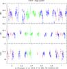 |
Fig. 1 UVOT magnitudes of WR 21a as a function of phase. Data from 2013 are shown with empty red triangles, data from 2014 with empty green squares, and data from 2015 with empty blue pentagons. |
2.2.3. Chandra
The Chandra X-ray facility observed serendipitously WR 21a with ACIS-I in April 2008. The system appears far off-axis, near a CCD edge. Consequently, the PSF is heavily distorted and the counts are spread over a large area, which avoids the pile-up of the source. The spectrum of WR 21a was extracted in a circle of radius 24.̋3 centred on its Simbad coordinates, that of the background in a nearby region of the same size and devoid of sources. Dedicated ARF and RMF response matrices were calculated via specextract (CIAO v4.7 and CALDB v4.6.9). The X-ray spectrum was binned in a similar manner to the XMM-Newton spectra. Count rates in the same energy bands as for XMM-Newton and Swift data were derived from the ungrouped spectrum using Xspec (see Table A.1) – they are thus not equivalent on-axis values.
3. The WR 21a system
The star now known as WR 21a was first detected as an Hα-emitter, appearing in the The (1966) catalogue under the name THA 35-II-042 and in the early-type emission-line star catalogue of Wackerling (1970) as Wack 2134. The star is situated to the east of Westerlund 2 (see e.g. Fig. 3 of Roman-Lopes et al. 2011) but its relation to that cluster remains unknown. In fact, the exact distance to the star is currently unknown, and even a precise V magnitude is lacking for WR 21a. Wackerling (1970) provides a value V = 12.8 whereas the more recent UCAC4 gives V = 12.67 (Zacharias et al. 2013). In our spectra, we note that the interstellar Na i D lines have components with velocities from –12 km s-1 to +10 km s-1. Adopting the Galactic rotation law of Fich et al. (1989), we then deduce a kinematical distance of about 5–5.4 kpc which is in between the small (~2.6 kpc, Ascenso et al. 2007; Ackermann et al. 2011) and large (~8 kpc, Rauw et al. 2011) distance values of the Westerlund 2 cluster, but similar to the middle determination of Fukui et al. (2009) and Vargas Álvarez et al. (2013). The interstellar K i λ7699 and CH λ4300 lines exhibit the local absorption component up to +10 km s-1 on the red side but display nothing on the blue side.
Figure 2 shows the spectrum of WR 21a in the region of the diffuse interstellar band (DIB) at 8621 Å. We measured an equivalent width of 0.42 Å for this feature. Following the calibration of Wallerstein et al. (2007), this corresponds to an excess E(B−V) = 1.8 in good agreement with the conclusion of E(B−V) = 1.48−1.9 from Caraveo et al. (1989). Another estimate can be calculated from the JHK magnitudes of the system from 2MASS data. Correcting these magnitudes to the standard system, we derived (J−H) = 0.664 and (H−K) = 0.343. Dereddening the (J−H) colour to the typical colour of massive O-stars, we deduced an equivalent excess E(B−V) = 1.6 to 2.0. The same exercise was made considering both the (J−H) and (H−K) intrinsic colours of a WN5h star as calibrated by Rosslowe & Crowther (2015), which yields E(B−V) = 1.7 to 1.9, further supporting the above-mentioned value of 1.8 for this excess. We thus adopt this value for the present work. Using the calibration of Bohlin et al. (1978) and Gudennavar et al. (2012), this colour excess corresponds to an equivalent hydrogen column density of 1022 cm-2.
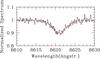 |
Fig. 2 Mean FEROS spectrum of WR 21a around the DIB at 8621 Å. The red curve gives the fit by a Gaussian function of dispersion σ = 1.78 Å. |
3.1. WR 21a as a high-energy source
WR 21a was tentatively identified as the optical counterpart of the X-ray source 1E 1024.0–5732 from the Einstein Galactic Plane Survey (Hertz & Grindlay 1984). It was then suggested that this X-ray source was not coronal in nature, as in sun-like stars. In addition, this X-ray source was amongst a small group of objects present in the error box of the γ-ray source 2CG 284–00 (Caraveo 1983; Goldwurm et al. 1987). A few years later, Caraveo et al. (1989) confirmed the association of the X-ray source with the early-type star but also reported the detection of a 60 ms pulsation in the X-ray emission that they considered reminiscent of a pulsar. They thus concluded that it was a O+neutron star binary. However, Dieters et al. (1990) discarded the presence of any pulsation in the visible domain and Belloni & Mereghetti (1994) were also unable to find support for the 60 ms pulsations in ROSAT observations. In parallel, observations in the visible domain instead suggested that the optical spectrum was of the type WN6 (or WN5) with a possible companion. This made Wack 2134 the first Wolf-Rayet star discovered thanks to its X-ray emission (Mereghetti & Belloni 1994; Mereghetti et al. 1994, 1995).
Using the Rossi X-ray Timing Explorer, Reig (1999) analysed the 3–15 keV spectrum of 1E 1024.0–5732. He concluded that it was a rather soft source (hence not an accretor), clearly favouring a colliding wind scenario rather than the HMXB scenario. He further refuted the presence of any rapid fluctuations but mentioned that the source is probably variable on timescales of years. WR 21a has also been observed with the ASCA Gas Imaging Spectrometer and appears as the faint and low-variability source AX J1025.9–5749 in the catalogue of Roberts et al. (2001). In addition, WR 21a is, in the radio domain, a possible non-thermal emitter (Benaglia et al. 2005; De Becker & Raucq 2013), which is another possible characteristic of colliding winds.
 |
Fig. 3 Relative orbit of the O-star in WR 21a around the Wolf-Rayet primary star. The orbit is projected on the plane defined by the line of sight (vertical dashed line) and the line of nodes (horizontal dashed line). This was calculated according to the orbital solution of Tramper et al. (2016) with an assumed inclination of 58.̊8. Both axes are in units of the solar radius; the Earth is located to the bottom at y = −∞ on the ordinate axis. The orbital motion is counterclockwise. Open circles indicate the position of the O-star between phases 0 and 1 by step of 0.1. Periastron (P) occurs at phase φ = 0.0 and apastron (A) at φ = 0.5. The filled circles indicate the binary configuration at each of the XMM-Newton observations. The passages through the lines of nodes (horizontal dashed line) occur at φ = 0.0335 and φ = 0.928, whereas the conjunctions (intersections between the orbit and the vertical dashed line) occur at φ = 0.316 and φ = 0.9935. |
3.2. WR 21a as a binary system
Despite the suspicion of binarity from the high-energy studies, the characteristics of WR 21a remained poorly known until recently. The first detailed analyses by Niemela et al. (2006) and Niemela et al. (2008) definitively proved that WR 21a is actually a binary system with a period of 31.673 d and a large eccentricity. The absence of He i lines for the O companion indicated an early O3–O4 star, whilst the spectral type of the WR was estimated to WN6. Quite recently, the system has been densely monitored with X-Shooter at ESO’s VLT by Tramper et al. (2016). They broadly confirmed the previous results and improved the orbital solution. We adopt this latter solution (Table 2 and Fig. 3). The spectral types were revised to O3/WN5h+O3Vz((f∗)).
The orbital solution indicates rather large minimum masses (Msin3i of 65.3 M⊙ for the WN star and 36.6 M⊙ for the O companion), putting WR 21a in the list of very massive systems with a WNLh primary (like WR 22, WR 20a, WR 25, and WR 29; see respectively Rauw et al. 1996, 2005; Gamen et al. 2006, 2009). The inclination is basically unknown, but if a mass of 58 M⊙, typical of O3V stars (Martins et al. 2005) is attributed to the O-type companion, an inclination i = 58.̊8 is deduced, leading to a high mass of 104 M⊙ for the WN5h star (Tramper et al. 2016). WR 21a would thus be one of the rare examples of the most massive stars (M ≳ 100 M⊙), underlining its interest.
The ephemeris derived by Tramper et al. (2016) were used for deriving the phases of the X-ray observations (see Table A.1). They are precise: The error on the reference time of periastron amounts to 0.32 d, inducing a possible error on the phase of 0.01; the error on the period (0.013 d) turns out, over five cycles, to an error on the phase of 0.002 only. Nevertheless, to be sure that the phases derived for our XMM-Newton data are correct, we measured the radial velocities of the He ii λ5412 line of both objects on the contemporaneous optical spectra. Comparing them with the predictions from the orbital solution of Tramper et al. (2016, see also Fig. 4, we found that the error on the phases is not larger than 0.01. Uncertainties should be slightly larger for Swift observations taken in 2014 and 2015 as well as for the Chandra 2008 spectrum, as the reference time of periastron in Tramper et al. (2016) is in 2013 and there are about 11−12 cycles per year, but errors on the phases should nevertheless remain below 0.05 for Swift and 0.12 for Chandra. This is confirmed by the near-perfect reproduction of the X-ray light curve with time (see next section).
Physical parameters of WR 21a.
Despite these previous studies, the stellar and wind parameters are still largely unknown. This is notably owing to the lack of a detailed study of the WN spectrum with stellar atmosphere codes such as e.g. CMFGEN (Co-Moving Frame GENeral, Hillier & Miller 1998). The second part of Table 2 thus yields parameters, such as star radii and mass-loss rates, which are inspired from several studies of similar objects. Considering the primary star, we used the analysis of equivalent WN5-6(h) stars by Crowther et al. (1995) and Hamann et al. (2006) as well as the parameters of the WN7ha star WR 22 (Gosset et al. 2009; Gräfener & Hamann 2008) and of the WN6ha star WR 20a (Rauw et al. 2005). Parameters for the O companion come from the calibration of Martins et al. (2005) and of Muijres et al. (2012). Whilst they should certainly not be taken at face value, these parameters can be considered as representative, helping to get a first idea of the nature of the wind-wind collision; these parameters suggest that the wind momentum of the WR star is overwhelming the one of the O-star. Under the hypothesis of instantaneously accelerated winds, we expect the apex of the collision to be on the binary axis at 73% of the system separation from the WR, i.e. close to the O-star. If we further consider some radiative braking acting on the WR wind, the apex moves away from the O-star. Using the formalism of Gayley et al. (1997, see their Eq. (4)), the apex might shift to 58% of the separation if we adopt a maximum value of about two for the reflection factor S. If instead we consider a radiatively accelerated wind obeying a classical β-velocity law (e.g. β = 0.8 for both stars), we still find a value of 73% (neglecting the braking) for the apex position during the major part of the orbit (roughly from phase 0.2 to 0.8). Around periastron, it appears that the O-star wind could have difficulty in supporting the WR wind with, hence, a possible crash on the surface of the O-star. However, this possibility is attenuated if braking is considered. In particular, the maximum value of S corresponds to an ability for the O-star to fully sustain the WN wind, restoring the position of the apex at 57%.
 |
Fig. 4 Radial velocity curves for both components in WR 21a from the orbital solution of Tramper et al. (2016). The dashed blue and continuous red lines provide the curves for the secondary and primary, respectively. The dots represent the RVs measured on the 2013 FEROS spectra acquired contemporaneously with the XMM-Newton data. The agreement with the pre-established orbital solution is good. The error-bars represent 1σ standard deviation. |
 |
Fig. 5 Light curves of the four XMM-Newton observations (pn in green, MOS1 in black, MOS2 in red). For each exposure, the top (resp. bottom) panels show the light curves with 200 s (resp. 1000 s), whilst the left, central, and right panels display the total, soft, and hard light curves, respectively. The ordinates are in count/s: on the left side for the total light curves, on the right side for the soft and hard light curves. |
The nature of the collision can be derived from the value of the index χ, which represents the ratio of the typical cooling time over the escaping time (Stevens et al. 1992). For solar abundances, we have  , where v1000 is the pre-shock velocity in units of 1000 km s-1, d12 is the star-apex separation in units of 107 km, and Ṁ-7 is the mass-loss rate in units of 10-7 M⊙ yr-1. For our adopted values, it is in the range 0.3−40 for the O-star (depending on the actual location of the apex, on the considered phase, and on the actual inclination of the system) but it is always less than 0.35 for the WR (taking into account the WN abundances). The post-shock O wind thus is in an intermediate state between radiative and adiabatic behaviours, but on the adiabatic side, whereas the shocked WR wind is at best in an intermediate state, but on the rapidly cooling side. Therefore, one could expect a weakly varying hard component and instabilities a little more developed than in the case of WR 22 (Parkin & Gosset 2011). We are now going to check these ideas by analysing the results of the XMM-Newton observations.
4. The X-ray emission of WR 21a and its CWR
Significance levels (in %) associated with χ2 tests for constancy of the background-corrected XMM-Newton light curves with 1 ks bins.
 |
Fig. 6 Variation of the count rates and hardness ratio with orbital phase, for XMM-Newton (in black dots), Chandra (filled black triangle), and Swift data (empty red triangles for 2013, empty green squares for 2014, and empty blue pentagons for 2015). For all energy bands, Chandra and Swift count rates and their errors were multiplied by 5.4 and 19, respectively, to clarify the trends, and no further treatment was made for adjustment. To help compare with physical parameters, the bottom left panels provide the orbital separation (in units of the semimajor axis a) as well as a position angle defined as zero when the WR star is in front and 180° when the O-star is in front. The vertical dotted lines in the left panels thus correspond to the quadratures and the other dotted line to an arbitrary 1 /D variation (not fitted to the data); periastron occurs at φ = 0.0. |
4.1. The light curves
The good sensitivity of XMM-Newton allows us to search for variations within the exposures (Fig. 5). We note that differences are expected between instruments as pn and MOS do not have the same spectral sensitivity and do not receive the same amount of photons; about half of the flux in front of MOS telescopes is redirected into the reflexion grating spectrometer (RGS) leading to larger noise in MOS data. Besides, noise makes light curves recorded even by twin-like instruments that are not exactly identical (for more discussion and examples, see Nazé et al. 2013). All these problems can however be overcome by cautious statistical testing. As for ζ Pup (Nazé et al. 2013), the same set of tests was applied to all cases. We first performed a χ2 test for three different null hypotheses (constancy, see e.g. Table 3; linear variation; quadratic variation), and further compared the improvement of the χ2 when increasing the number of parameters in the model (e.g. linear trend vs constancy) by means of Snedecor F tests (nested models, see Sect. 12.2.5 in Lindgren 1976). Adopting a significance level of 1%, we found that WR 21a has not significantly varied during the first XMM-Newton observation, but that the hard pn light curve with 1 ks time bins in the second XMM-Newton observation is found to be significantly variable and significantly better fitted by a linear relation. In the third XMM-Newton observation, the pn and MOS2 light curves in the total energy band are significantly better fitted by linear or quadratic relations than by a constant whilst the MOS1 light curve appears significantly variable. Finally, in the last observation, WR 21a always appears significantly variable and better fitted by linear or quadratic relations. Indeed, a decrease of the count rate is obvious in the last two XMM-Newton observations (Fig. 5), although it is shallower for the former one of these last two.
To put these results into context, we also looked at the global light curves, i.e. light curves combining XMM-Newton, Chandra, and Swift data, with one point per exposure (Fig. 65). Variations recorded by these observatories agree well, even if they are several cycles apart. Moreover, it is obvious that the last two XMM-Newton observations were taken when WR 21a becomes fainter, explaining the above results. In fact, the brightness of WR 21a does not change much from φ = 0.2 to 0.7, but important variations are seen between φ = 0.8 and 1.1, i.e. around periastron passage. First, the count rate increases, by about 80−100% with a maximum before conjunction and periastron (at φ ~ 0.9). Next, a sharp drop in the soft band is detected with a minimum reached slightly before φ ~ 0.0, most probably at conjunction (which occurs at φ ~ 0.9935). Despite the fact that the hard band must be much less sensitive to absorption effects, a drop is also observed in this band. Moreover, the amplitude of the drop does not strongly depend on energy. The count rates at minimum are about four times smaller than these at φ = 0.2−0.7. In parallel, the hardness ratio increases from φ = 0.95 up to φ ~ 0.0 but comes back to its original value after that. This suggests that the minimum occurs slightly later in the hard band than in the soft band. It may be noted that the behaviour of the light curve appears more complicated than a simple eclipse by the WR near φ ~ 0.9935. Also, there is clearly no eclipse when the O-star is in front (around φ = 0.316), as would be expected for large inclination systems (e.g. V444 Cyg, Lomax et al. 2015).
Finally, the increase in the count rate before periastron appears to follow a 1 /D trend (see dotted line in Fig. 6), typical of adiabatic systems (where χ ≫ 1). In fact, this trend can actually be detected from φ = 0.2 to φ = 0.9. This point is discussed further below.
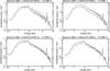 |
Fig. 7 Variation of the shape of the XMM-pn spectra with time, each panel showing an individual spectrum. In each panel, we also superimposed the best-fit model (absorbed 2T model with individual absorption columns) of the preceding (in phase) pn spectrum (see Sect. 4.2). |
4.2. The spectra
Results of the spectral fits of XMM-Newton observations above 3.0 keV.
Results of the spectral fits of XMM-Newton observations over the whole energy range (0.3–10.0 keV).
4.2.1. Look at the XMM-Newton spectra
The four XMM-Newton pn spectra are shown in Fig. 7 to facilitate the inspection of the changes. With each pn spectrum, the best-fit model of the pn spectrum preceding it in phase is also shown (see Sect. 4.2.2). A simple visual inspection of the spectra confirms the changes seen in the light curves. When going from the first to the second spectrum, it is evident that the star brightens. The increase occurs in a very similar way (in log flux scale) over the full energy range. Going from the second to the third spectrum, the star overall becomes fainter, but this time there are changes with energy; the hard tail (above 3.0 keV) still exhibits a small increase in flux whilst a strong decrease is seen at lower energies (below 2.0 keV), suggesting an effect of absorption. As the star becomes even fainter (fourth observation), even the hard part of the spectrum starts to decline. Going from the fourth observation to the first, the star is still faint in the hard band whereas it is brighter below 1.5 keV. Looking at Swift and Chandra spectra confirms these trends, but also reveals the absence of large spectral changes at phases φ = 0.2−0.8 as well as the progressive recovery of the soft flux at φ = 0.0−0.1. To pinpoint these changes, the spectra were fitted within Xspec v12.8.2 (Dorman & Arnaud 2001) assuming solar abundances of Asplund et al. (2009) and cross-sections of Balucińska-Church & McCammon (1992; with changes from Yan et al. 1998, i.e. bcmc case within Xspec).
4.2.2. Analysis of the XMM-Newton spectra
In general, we studied the MOS1, MOS2, and pn spectra as well as their combination over the three detectors. For the sake of simplicity, in the following, we limit the description of our results to the combined datasets. As a first step, we studied the spectra restricted to above 3.0 keV. In this region, only a very huge absorbing column could produce some effect. This provides the opportunity for a detailed study of the hard band. We considered a powerlaw model, and a Gaussian function for the Fe-K line. The results are given in the top of Table 4. The simultaneous fits to pn and MOS spectra with this model indicate no significant change in slope, which is entirely compatible with the 2.8 value reported by Reig (1999). Moreover, the position of the Fe-K line is derived to be in the range 6.67−6.72 keV. The transitions corresponding to weakly ionised iron should rather be situated around 6.4 keV. A line located above 6.6 keV implies that the ion should at least be Fe xxiii. The most likely dominant origin is the Fe xxv ion as suggested in Rauw et al. (2016). This indicates that the plasma is highly ionised, as expected from strong shocks in a CWR. As the presence of this line indicates that the hard X-rays originate in a very hot plasma rather than through non-thermal processes, we also fitted a mono-temperature unabsorbed apec model (see bottom part of Table 4). Although the derived temperature gradually shifts from 3.2 keV to 2.8 keV when going from spectra XMM-1 to XMM-4, the change is not significant (difference less than 3 individual σ) and we can conclude that the hot component does not strongly vary in temperature. Therefore, the marked variability of the hard flux is not due to changes in the shock temperature.
 |
Fig. 8 Variation with orbital phase of the spectral fit parameters and fluxes (see Table 6 for details). Black dots correspond to XMM-Newton spectra, the cyan filled triangle to the Chandra spectrum, and magenta crosses to binned Swift spectra (see text). Left panel: absorption, normalisation factors, and observed fluxes. Right panel: ISM-absorption corrected fluxes, in both the 0.5–2.5 keV and 2.5–10.0 keV energy bands, as a function of phase (top) and separation (bottom). |
The XMM-Newton spectra were also fitted over the whole energy range (0.3−10.0 keV) with two-temperature thermal plasma models that are optically thin. Again, all three XMM-Newton-EPIC spectra of a single observation were simultaneously fitted. We first considered a common absorbing column in front of the two thermal components. Alternatively, we considered a model with separate absorbing components in front of the emitting components. The results are presented in Table 5. In the former case (common absorbing column), the warm component has a temperature of ~3.0 keV whereas in the latter case (individual columns), the fits are less secure and the warm temperature is around 2.3 to 3.6 keV, but both values are in good general agreement with previous results. Concerning the low-temperature component, the temperature is also stable and near 0.8 keV. The fits with individual absorptions appear better, although the difference is only significant for pointing XMM-4. The absorbing column density in the common absorption fits seems to vary from 0.4 to 1.2 × 1022 cm-2 but the increase is less marked for the absorbing column in front of the soft emitter in the two-column fits (0.4 to 0.9 × 1022 cm-2). In these two-column fits, the absorbing column in front of the hard component is not very well defined, as could be expected in view of the lower sensitivity to this parameter, but it appears to reach higher values than those in front of the soft component (up to ~3 × 1022 cm-2). Clearly, the strongest variations with phase appear in the intrinsic strength of the components, as traced by the EM (or, equivalently, the normalisation factors of the apec models). From phase 0.57 to 0.89, the EM increases by 50% for the soft component and by 100% for the hard component. From phase 0.89 to 0.95, the EMs are still increasing by a few tens of percent. Finally, from phase 0.95 to 0.97, the EMs for the soft component are decreasing, but the behaviour associated with the hard one is less marked. The decrease in hard flux between XMM-3 and XMM-4 can be interpreted as due to a variation of the absorbing column by an amount of a few 1022 cm-2. It should, however, be noted that the decrease in the hard flux between the pointings XMM-3/XMM-4 and the Swift observation at minimum (00032960018, see Table A.1; also labelled Swift-A, see Table 6) is much larger. It can be reproduced by fixing the norm factor and increasing the attenuation in front of the hot component by some 3.−4. × 1023 cm-2. This is not however the natural best-fit situation (which favours a decrease of the EMs; see Table 6). In addition, such a large column is not very likely; at least, it should induce a slope effect inside the 2.5−7.0 keV range. This effect is not seen on the Swift-A spectrum. However, we must admit that the very low quality of these Swift data does not provide a strong constraint. A firmer conclusion would be obtained by the future acquisition of an XMM-Newton observation at periastron. Therefore, we conclude with some caution that a column increase alone could not be invoked to explain the decrease in flux from φ = 0.95 to φ ~ 0.0, and that a decrease of the intrinsic strength is necessary (i.e. a change in the quantity of emitting material as traced by the emission measure EM). We thus suggest, in good agreement with the various fits, that the dip in the X-ray light curve around periastron is due to a combination of an increase of the absorbing column density and of a decrease of the EM.
Finally, we should mention that freeing abundances of HeCNO (as the WR component may have non-solar abundances) for either the emission or the absorption component neither improves the fits nor changes the trends significantly, hence, we restrict the discussion to the solar case.
4.3. Analysis of the whole dataset
All the X-ray spectra were fitted within a general scheme comprising a common model. Since the signal to noise of the individual Swift spectra are very low (about 80–150 raw counts), we defined 12 phase bins (0.0–0.05, 0.05–0.1, 0.1–0.2, 0.2–0.3, 0.3–0.4, 0.4–0.5, 0.5–0.6, 0.6–0.7, 0.7–0.8, 0.8–0.9, 0.9–0.95, and 0.95−1.0) and simultaneously fitted the spectra taken within the same phase bin. For fitting all these spectra, two thermal components are sufficient to provide a good fit, as shown before for XMM data. Temperatures of about 0.8 and 3.0 keV were always found, hence, we decided to fix the temperatures to these values. However, it must be noted that models with individual absorptions proove too erratic when fitted on the noisier Swift spectra, so we restricted ourselves to the common absorption model for these data (it clarifies the trends). Fitting results are provided in Table 6 and shown graphically on Fig. 8. There are some small differences between Swift, Chandra, and XMM-Newton results, probably because of noise and remaining cross-calibration effects, but these differences remain well within errors.
Fluxes and normalisation factors mirror the trends seen in the count rates with an increase before periastron, then a sharp drop, and finally a slow recovery (Fig. 8). It should be particularly underlined that these variations are not restricted to the cooler emission component or the softest flux, despite the fact that hard X-rays are much less influenced by absorption effects. In addition, looking at normalisation factors, it is also clear that the maximum intrinsic emission occurs near the third XMM-Newton observation (φ ~ 0.95). If the maximum observed soft flux (or count rate) occurs in the second observation (φ ~ 0.89), this is solely due to the increased local absorption, which significantly decreases the soft flux (indeed, the maximum hard flux occurs near φ ~ 0.95).
Local absorption indeed varies, especially at phases 0.9–1.1. The maximum is recorded at φ ~ 0.0 with at least a tripling of the value corresponding to the passage of the WR star in front of the system (Table 6 and Fig. 8). When two individual absorptions are used (see bottom of Table 6), they are similar at first, but that of the hotter component increases more rapidly towards periastron than that of the cooler component. This agrees well with CWR models (Pittard & Parkin 2010), which predict the generation of hard X-ray flux deeper in the winds, near the line of centres (whilst soft emission may arise further downwards of the shock cone).
It must be noted that these variations are not symmetrical around periastron. First, the decline in intrinsic emission begins before periastron. Second, the increase in absorption occurs more rapidly than the decrease. This leads to an interesting hysteresis effect (see right panels of Fig. 8), which is very similar to predictions of Pittard & Parkin (2010, see next section for a discussion).
5. Discussion
The X-ray monitoring of WR 21a brought several important results. We now summarise and tentatively interpret them, also pointing out the remaining open questions. Although the orbit of WR 21a is rather well determined, this is far from the case for the other properties of the two components (mass-loss rates, radii, ....) as already mentioned in Sect. 3.2. In this context, the discussion could only be considered as preliminary. We divided the discussion into four basic topics.
5.1. The X-ray light curve from phase 0.2 to 0.9
As mentioned in previous sections, the X-ray light curves seem to exhibit a 1 /D flux variation (where D is the instantaneous separation between both stars). The similarity of the observed variations with a 1 /D trend is so high that it is unlikely that it could be a chance effect. The separation at φ = 0.5 is 1.694 × a (with a the semimajor axis of the orbit) and that at φ = 0.9 is 0.812 × a. The ratio between separations amounts to 2.08, which agrees well with the above-mentioned 100% increase in fluxes and count rates between these phases. Such a 1 /D behaviour is expected when cooling of the post-shock gas is adiabatic (Stevens et al. 1992). The effect arises because the emission volume scales as D3 whilst the emissivity per unit volume goes as the square of the density and this density (pre-shock and post-shock) scales as Ṁ/D2, as explained by Stevens et al. (1992, see their sect. 3.1 and Eq. (10)). Such a 1 /D trend was detected in some long-term WR+O systems like WR 140 (period of 7.9 years; Corcoran et al. 2011) and WR 25 (period of 208 d; Gosset 2007; Güdel & Nazé 2010; Pandey et al. 2014) but it was not observed in the complex case of WR 22 (period of 80 d; Gosset et al. 2009; Parkin & Gosset 2011).
However, based on the probable stellar and wind parameters (Table 2), the shocked WR wind in WR 21a should instead be on the rapidly cooling side (see Sect. 3.2) and this WR wind should dominate the emission (although this is still to be proven). The 1 /D behaviour is therefore somewhat unexpected. Nevertheless, this discrepancy could perhaps be understood considering the work of Zhekov (2012), which seemed to detect an adiabatic behaviour in a sample of close WR+O binaries. If plotted in Fig. 2 (right panel) of Zhekov (2012), WR 21a would be precisely located on the solid straight line expected for systems with a CWR in the adiabatic regime. Zhekov (2012) concludes that the phenomenon making short-period systems exhibit an adiabatic behaviour could be due to the clumpy nature of the wind.
An alternative possibility could perhaps be the fact that the companion wind is adiabatic. As shown in Parkin & Gosset (2011), in the case of the preliminary models of WR 22, the thermal pressure of the O wind in the post-shock region acts like a cushion for the contact discontinuity. This has two effects. First, the contact discontinuity does not change its general structure. Second, this cushion prevents the thin-shell instabilities (generated by e.g. the radiative cooling of the WR wind) from growing in a non-linear manner. In such a case, one could imagine that instabilities in the WR wind are damped and, hence, not strong enough to destroy the above-mentioned density effect leading to the 1 /D behaviour. Only detailed 3D hydrodynamical simulations could perhaps elucidate this surprising observation but such simulations are well beyond the scope of the present paper.
5.2. The X-ray light curve around periastron
In the regions of the light curve where the stars are approaching periastron, the flux of WR 21a exhibits a sudden decrease and a much slower recovery. Such a behaviour has been observed in WR 140 (Corcoran et al. 2011) and in η Carinae (Moffat & Corcoran 2009, and references therein). Is the present one of the same nature ? The minimum flux appears near φ ~ 0.9935 in the soft band. This phase corresponds to conjunction (with the WR star in front) and thus to a possible eclipse. The typical width at half depth of the observed dip is 0.07 (in phase). A core-core eclipse would span a time corresponding to a maximum of δφ = 0.01−0.015. In order to generate the wider dip that is observed, the CWR would have to be more extended than the O stellar core, which is certainly possible. However, only part of the CWR would then be eclipsed by the small WR core at a given phase, failing to reproduce the strong decrease in hard flux. In addition, the absence of eclipses is noted in the UV light curve (see Fig. 1), yielding support for a low inclination angle. Moreover, the favoured inclination derived from the orbital solution and typical masses of O-stars (58.̊8) would also prevent eclipses from occurring. Therefore, the decrease of the X-ray fluxes should be linked to a phenomenon with a longer lasting effect, such as an increase of absorption along the line of sight due to the dense WR wind, as also suggested by Fig. 6. However, we should note that the WR is the star closer to the observer between φ = 0.928 and 0.0335, whilst the minimum flux episode occurs from φ = 0.95 to 0.15. This is a large difference; a Coriolis effect is probably not able to fully explain it, but detailed simulations need to be performed to pinpoint the extent of the problem.
The corresponding minimum in the hard band occurs at φ = 0.0. As explained in Sect. 4, it is more difficult to explain by absorption since it would necessitate an extremely large column of 3.−4. × 1023 cm-2 as a result of the much lower sensitivity of the hard X-rays to photo-absorption. Such a huge column density is unlikely even if it is now generally admitted that the structure of WR winds very close to their hydrostatic surface is not properly described by the current models. Therefore, another cause is responsible for the hard X-ray flux decrease. The minimum in the hard band essentially corresponds to a decrease of the EMs. An apparent decrease of the EM could be obtained through a core-core eclipse phenomenon but, as already stated above, this hypothesis is unlikely. On the other hand, the stability of the colliding zone may be questioned: when stars are close to each other, a stable CWR may not be reached, and the stronger wind may then push the CWR to the vicinity of the O-star; this leaves less room for the O-star wind to accelerate. This would lead to a crash of the WR wind onto (or close to) the photosphere of the companion. The slow recovery after a disruption could further explain the slow rise of the fluxes after periastron (up to phase φ ~ 0.1−0.2 – for an illustration; see Model B of Parkin & Gosset 2011). The uncertainty on the efficiency of radiative braking does not permit us to be predictive without a detailed modelling but, using the parameters from Table 2, the WR wind could overwhelm the O wind starting around phase 0.8−0.9. However, the disruption of the CWR should lead to the disappearance of the hard flux, as predicted by hydrodynamical simulations (Parkin & Gosset 2011). Here, on the contrary, WR 21a just becomes fainter; its hard X-ray flux never completely disappears.
Figure 8 shows that the variation of the fluxes with stellar separation presents a strong hysteresis. Such a phenomenon has been observed in several systems (see e.g. the case of Cyg OB2#8 in Cazorla et al. 2014). Theoretically, this effect has been detected by Pittard & Parkin (2010) when analysing the light curve of their model labelled cwb4. Considering only the expected changes in luminosity of a CWR in the adiabatic regime because of the changing orbital separation and true wind velocity at the shock, Sugawara et al. (2015) demonstrated that only at most half of the amplitude of the hysteresis phenomenon can be quantitatively explained; an additional effect is needed to explain its full extent, in particular, the region of the central dip. Moreover, an apparent change in wind velocity along the orbital cycle should induce a change in the shocked plasma temperature. This expected change is not observed in the data, suggesting that it is not the solution. An instability leading to a disruption (at least partial) thus seems necessary to explain the full extent of the hard band variations.
To explain both the soft and hard band variations of WR 21a, both absorption and partial disruption are thus necessary. The disruption is usually marked, however, by a net softening of the X-ray emission that is not present in WR 21a. All this should, however, be further studied and confirmed using detailed 3D hydrodynamical simulations.
5.3. The X-ray light curve around φ = 0.316
Phase φ = 0.316 corresponds to the conjunction with the O-star in front. At that particular moment, the cone formed by the CWR is mainly directed towards the observer. If the density of the O-star wind is lower, which is almost always the case, then there is less absorption along the line of sight and the shock zone is better seen through the O-star wind than during the remaining parts of the orbit. This should be accompanied by an apparent brightening of the X-ray luminosity. However, this effect is only observable if the line of sight from the apex towards the observer lies within the shock cone and this is only possible if the complement of the inclination of the system is less than half the opening angle of the CWR. The X-ray light curve of WR 21a does not show any variation of this kind at that particular phase, reinforcing the conclusion that large inclination values are excluded for this system.
5.4. The expected absorbing column density
Just before periastron, the absorbing column along the line of sight from the apex of the CWR to the observer reaches a maximum (see e.g. Fig. 8). On the basis of the adopted parameters given in Table 2, we can calculate a theoretical equivalent hydrogen column by integrating the wind densities found around the WR star (as a function of distance to that star) along the line of sight from the expected position of the apex to a point far away enough from the WR that the wind no longer contributes significantly to the column. The computed density column is then corrected by XH/mH, where the numerator is the abundance in mass of hydrogen and the denominator the mass of the H atom. We thus obtain an equivalent NH. Figure 9 shows, for an inclination of 58.̊8 (see Sect. 3.2), the evolution of the theoretical column as a function of phase. The figure also exhibits the observed values as derived above. To agree with these observed columns (derived from the XMM-Newton data), the theoretical mass-loss rate of the WR star would have to be reduced to ~ 1 × 10⁻⁵ M⊙ yr-1 at a first level of approximation. This result remains true even for non-solar abundances typical of WNLh stars, as fitting trials with different column models (solar composition versus that of WR 22) yielded similar column values, taking the different XH into account. However, no effort has been made to include the extent of the emitting region in this calculation and a definitive answer on WR 21a mass-loss rate should await confirmation by sophisticated hydrodynamical simulations.
 |
Fig. 9 Variation with phase of the equivalent hydrogen column density along the line of sight from the apex. The column is computed according to the physical parameters given in Table 2 and for an inclination of 58.̊8. We show the curves expected for various mass-loss rates: 0.5 × 10⁻⁵ M⊙ yr-1 (lower curve), 1.0 × 10⁻⁵ M⊙ yr-1 (middle curve), and 3.2 × 10⁻⁵ M⊙ yr-1 (upper curve, value adopted in Table 2). The figure also includes (open circles) the four values for the common column fits deduced from the XMM-Newton observations. In addition, the two filled squares indicate the column in front of the sole hard component for the XMM-3 and XMM-4 pointings. |
6. Conclusion
WR 21a is a very interesting system as it contains a WNLh star, which turns out to be very massive and is a key point to understanding massive star evolution. To learn more about the winds in this system, we have studied its wind-wind collision in X-rays using XMM-Newton as well as archival Chandra and Swift datasets.
The EPIC spectra are well fitted by a two-component, optically-thin thermal plasma model suggesting as temperatures 0.8 keV and 3.0 keV. These temperatures are rather well defined and present almost no change. The situation appears very different when examining the X-ray fluxes. From phase φ = 0.2 to 0.8, the fluxes do not vary much but then they increase and at φ = 0.9 reach a level twice that at φ = 0.5. The highest observed flux, in the band 0.5–10.0 keV, amounts to  erg cm-2 s-1, and the maximum flux in the same band, corrected for the interstellar absorption, is
  erg cm-2 s-1. This leads to a luminosity
  d2 erg s-1, if d is the distance to the star given in kpc. Assuming a distance of 5.2 kpc, this leads to a luminosity of 3.0 × 1034 erg s-1, placing WR 21a amongst the brightest WN + O systems, along with e.g. HD 5980 (
 erg s-1; Nazé et al. 2002) and WR 25 (
 erg s-1; Pandey et al. 2014); for comparison, WR 22 and WR 20a are one order of magnitude fainter (Gosset et al. 2009; Nazé et al. 2008). These conclusions are highly dependent on the adopted values for the individual distances, however.
From φ = 0.2 to φ = 0.9, the X-ray light curve seems to follow a 1 /D trend, suggesting the CWR cools adiabatically whilst a radiative collision is expected. This result is however in line with the conclusions reached by Zhekov (2012). After φ = 0.9, the flux starts to decrease rather rapidly, reaching a minimum in the soft band at the time of the conjunction with the WR star in front. In the hard band, the minimum occurs slightly later, instead corresponding to the periastron passage, although the difference in phase of the two events is very small. The recovery from the minimum is slower than the decrease and ends at φ = 0.1−0.2. Eclipses cannot be considered a potential explanation for this variability, as several lines of evidence exclude a high inclination value: the duration of the X-ray flux minimum at periastron and the absence of increase in the X-ray flux at the conjunction with the O-star in front, the absence of eclipses in the UV domain, and the values of the stellar masses derived from the orbital solution. The observed decline in flux is then probably due to two phenomena. First, there is a strong absorption as the WR and its dense wind appear in front. This mostly affects the soft band and the X-ray spectral fits can then be used to constrain the mass-loss rate of the WR; we found a preliminary value of ~ 1 × 10⁻⁵ M⊙ yr-1. Second, the decrease in the intrinsic strength of the X-ray emission suggests a (partial) disruption of the shock, or even a crash of the CWR onto the photosphere of the companion, near or at periastron. After periastron passage, the recovery of the emission presents a strong hysteresis effect.
Now that the X-ray variations are well constrained, detailed atmosphere analysis of the UV/visible spectra and hydrodynamical simulations of the CWR are needed to further improve our understanding of this extremely massive system.
Since the discovery by the Einstein satellite that massive stars could be moderate X-ray emitters (Harnden et al. 1979; Seward et al. 1979), it appears that the observed X-ray luminosity of single OB stars is proportional to their bolometric luminosity with an observed ratio around 10-7 (Pallavicini et al. 1981; Seward & Chlebowski 1982; Berghöfer et al. 1997; Sana et al. 2006; Nazé 2009). This has been explained by the presence of shocks in the wind coming from instabilities due to its radiatively driven nature (Lucy & White 1980; Lucy 1982; Feldmeier et al. 1997a,b). For Wolf-Rayet stars, the situation is more complex: No detection of single WC star was reported in the X-ray domain (Oskinova et al. 2003); several single WN stars exhibit detectable X-ray emission (Skinner et al. 2010), whereas other WN stars remain undetected in this band (e.g. WR 40, Gosset et al. 2005).
SAS threads, see http://xmm.esac.esa.int/sas/current/documentation/threads/
In Fig. 6, Chandra and Swift count rates are multiplied by 5.4 and 19, respectively, whatever the energy band. This empirical correction does not rely on any theoretical assumption. It is only used to show in a simple way that all datasets agree throughout the whole orbit. However, the values of the applied factors agree well with what can be derived from simulations in Xspec (using fakeit and models of Table 6) and in PiMMS (for simpler emission models).
Acknowledgments
We acknowledge support from the Fonds National de la Recherche Scientifique (Belgium), the Communauté Française de Belgique, the PRODEX XMM-Newton and Integral contracts, and the “Action de Recherche Concertée” (CFWB-Académie Wallonie Europe). We thank Kim Page (Swift UK centre) for her kind assistance. ADS and CDS were used for preparing this document. We thanks H. Sana for a preliminary reduction of the FEROS data, and for having made his ephemeris available in advance of publication.
References
- Ackermann, M., Ajello, M., Baldini, L., et al. 2011, ApJ, 726, 35 [NASA ADS] [CrossRef] [Google Scholar]
- Ascenso, J., Alves, J., Beletsky, Y., & Lago, M. T. V. T. 2007, A&A, 466, 137 [NASA ADS] [CrossRef] [EDP Sciences] [Google Scholar]
- Asplund, M., Grevesse, N., Sauval, A. J., & Scott, P. 2009, ARA&A, 47, 481 [NASA ADS] [CrossRef] [Google Scholar]
- Balucińska-Church, M., & McCammon, D. 1992, ApJ, 400, 699 [NASA ADS] [CrossRef] [Google Scholar]
- Belloni, T., & Mereghetti, S. 1994, A&A, 286, 935 [NASA ADS] [Google Scholar]
- Benaglia, P., Romero, G. E., Koribalski, B., & Pollock, A. M. T. 2005, A&A, 440, 743 [NASA ADS] [CrossRef] [EDP Sciences] [Google Scholar]
- Berghöfer, T. W., Schmitt, J. H. M. M., Danner, R., & Cassinelli, J. P. 1997, A&A, 322, 167 [NASA ADS] [Google Scholar]
- Bohlin, R. C., Savage, B. D., & Drake, J. F. 1978, ApJ, 224, 132 [NASA ADS] [CrossRef] [Google Scholar]
- Caraveo, P. A. 1983, Space Sci. Rev., 36, 207 [NASA ADS] [CrossRef] [Google Scholar]
- Caraveo, P. A., Bignami, G. F., & Goldwurm, A. 1989, ApJ, 338, 338 [NASA ADS] [CrossRef] [Google Scholar]
- Cazorla, C., Nazé, Y., & Rauw, G. 2014, A&A, 561, A92 [NASA ADS] [CrossRef] [EDP Sciences] [Google Scholar]
- Corcoran, M. F., Pollock, A. M. T., Hamaguchi, K., & Russell, C. 2011, ArXiv e-prints [arXiv:1101.1422] [Google Scholar]
- Crowther, P. A., Hillier, D. J., & Smith, L. J. 1995, A&A, 293, 403 [NASA ADS] [Google Scholar]
- De Becker, M., & Raucq, F. 2013, A&A, 558, A28 [NASA ADS] [CrossRef] [EDP Sciences] [Google Scholar]
- Dieters, S. W., Hill, K. M., & Watson, R. D. 1990, Inf. Bull. of Var. Stars, 3500, 1 [NASA ADS] [Google Scholar]
- Dorman, B., & Arnaud, K. A. 2001, Astronomical Data Analysis Software and Systems X, ASP Conf. Proc., 238, 415 [NASA ADS] [Google Scholar]
- Feldmeier, A., Kudritzki, R. P., Palsa, R., et al. 1997a, A&A, 320, 899 [NASA ADS] [Google Scholar]
- Feldmeier, A., Puls, J., & Pauldrach, A. W. A. 1997b, A&A, 322, 878 [NASA ADS] [Google Scholar]
- Fich, M., Blitz, L., & Stark, A. A. 1989, ApJ, 342, 272 [NASA ADS] [CrossRef] [Google Scholar]
- Fukui, Y., Furukawa, N., Dame, T. M., et al. 2009, PASJ, 61, L23 [NASA ADS] [Google Scholar]
- Gamen, R., Gosset, E., Morrell, N., et al. 2006, A&A, 460, 777 [NASA ADS] [CrossRef] [EDP Sciences] [Google Scholar]
- Gamen, R., Fernández-Lajús, E., Niemela, V. S., & Barbá, R. H. 2009, A&A, 506, 1269 [NASA ADS] [CrossRef] [EDP Sciences] [Google Scholar]
- Gayley, K. G., Owocki, S. P., & Cranmer, S. R. 1997, ApJ, 475, 786 [NASA ADS] [CrossRef] [Google Scholar]
- Goldwurm, A., Caraveo, P. A., & Bignami, G. F. 1987, ApJ, 322, 349 [NASA ADS] [CrossRef] [Google Scholar]
- Gosset, E. 2007, Habilitation Thesis, Liège University, Belgium [Google Scholar]
- Gosset, E., Nazé, Y., Claeskens, J. F., et al. 2005, A&A, 429, 685 [NASA ADS] [CrossRef] [EDP Sciences] [Google Scholar]
- Gosset, E., Nazé, Y., Sana, H., et al. 2009, A&A, 508, 805 [NASA ADS] [CrossRef] [EDP Sciences] [Google Scholar]
- Gräfener, G., & Hamann, W. R. 2008, A&A, 482, 945 [NASA ADS] [CrossRef] [EDP Sciences] [Google Scholar]
- Güdel, M., & Nazé, Y. 2010, Space Sci. Rev., 157, 211 [NASA ADS] [CrossRef] [Google Scholar]
- Gudennavar, S. B., Bubbly, S. G., Preethi, K., & Murthy, J. 2012, ApJS, 199, 8 [NASA ADS] [CrossRef] [Google Scholar]
- Hamann, W. R., Gräfener, G., & Liermann, A. 2006, A&A, 457, 1015 [NASA ADS] [CrossRef] [EDP Sciences] [Google Scholar]
- Harnden, F. R. Jr., Branduardi, G., Elvis, M., et al. 1979, ApJ, 234, L51 [NASA ADS] [CrossRef] [Google Scholar]
- Hertz, P., & Grindlay, J. E. 1984, ApJ, 278, 137 [NASA ADS] [CrossRef] [Google Scholar]
- Hillier, D. J., & Miller, D. L. 1998, ApJ, 496, 407 [NASA ADS] [CrossRef] [Google Scholar]
- Kaufer, A., Stahl, O., Tubbesing, S., et al. 1999, ESO Messenger, 95, 8 [NASA ADS] [Google Scholar]
- Lindgren, B. W. 1976, Statistical theory, 3rd edn. (New York: McMillan Pub.) [Google Scholar]
- Lomax, J. R., Nazé, Y., Hoffman, J. L., et al. 2015, A&A, 573, A43 [NASA ADS] [CrossRef] [EDP Sciences] [Google Scholar]
- Lucy, L. B. 1982, ApJ, 255, 286 [NASA ADS] [CrossRef] [Google Scholar]
- Lucy, L. B., & White, R. L. 1980, ApJ, 241, 300 [NASA ADS] [CrossRef] [Google Scholar]
- Mahy, L., Gosset, E., Sana, H., et al. 2012, A&A, 540, A97 [NASA ADS] [CrossRef] [EDP Sciences] [Google Scholar]
- Martins, F., Schaerer, D., & Hillier, D. J. 2005, A&A, 436, 1049 [NASA ADS] [CrossRef] [EDP Sciences] [Google Scholar]
- Mereghetti, S., & Belloni, T. 1994, Mem. Soc. Astron. It., 65, 369 [NASA ADS] [Google Scholar]
- Mereghetti, S., Belloni, T., Shara, M., & Drissen, L. 1994, ApJ, 424, 943 [NASA ADS] [CrossRef] [Google Scholar]
- Mereghetti, S., Belloni, T., Haberl, F., & Voges, W. 1995, in Wolf-Rayet stars: Binaries, Colliding Winds, Evolution, eds. K. A. van der Hucht, & P. M. Williams, Proc. IAU Symp., 163, 481 [Google Scholar]
- Moffat, A. F. J., & Corcoran, M. F. 2009, ApJ, 707, 693 [NASA ADS] [CrossRef] [Google Scholar]
- Muijres, L. E., Vink, J. S., de Koter, A., et al. 2012, A&A, 537, A37 [NASA ADS] [CrossRef] [EDP Sciences] [Google Scholar]
- Nazé, Y. 2009, A&A, 506, 1055 [NASA ADS] [CrossRef] [EDP Sciences] [Google Scholar]
- Nazé, Y., Hartwell, J. M., Stevens, I. R., et al. 2002, ApJ, 580, 225 [NASA ADS] [CrossRef] [Google Scholar]
- Nazé, Y., Rauw, G., & Manfroid, J. 2008, A&A, 483, 171 [NASA ADS] [CrossRef] [EDP Sciences] [Google Scholar]
- Nazé, Y., Oskinova, L. M., & Gosset, E. 2013, ApJ, 763, 143 [NASA ADS] [CrossRef] [Google Scholar]
- Niemela, V. S., Gamen, R. C., Solivella, G. R., et al. 2006, Rev. Mex. Astron. Astrofis. (Ser. de Conf.), 26, 39 [NASA ADS] [Google Scholar]
- Niemela, V. S., Gamen, R. C., Barbá, R. H., et al. 2008, MNRAS, 389, 1447 [NASA ADS] [CrossRef] [Google Scholar]
- Oskinova, L. M., Ignace, R., Hamann, W. R., et al. 2003, A&A, 402, 755 [NASA ADS] [CrossRef] [EDP Sciences] [Google Scholar]
- Pallavicini, R., Golub, L., Rosner, R., et al. 1981, ApJ, 248, 279 [NASA ADS] [CrossRef] [Google Scholar]
- Pandey, J. C., Pandey, S. B., & Karnakar, S. 2014, ApJ, 788, 84 [NASA ADS] [CrossRef] [Google Scholar]
- Parkin, E. R., & Gosset, E. 2011, A&A, 530, A119 [NASA ADS] [CrossRef] [EDP Sciences] [Google Scholar]
- Pittard, J. M., & Parkin, E. R. 2010, MNRAS, 403, 1657 [NASA ADS] [CrossRef] [Google Scholar]
- Rauw, G., Vreux, J. M., Gosset, E., et al. 1996, A&A, 306, 771 [NASA ADS] [Google Scholar]
- Rauw, G., Crowther, P. A., De Becker, M., et al. 2005, A&A, 432, 985 [NASA ADS] [CrossRef] [EDP Sciences] [Google Scholar]
- Rauw, G., Sana, H., & Nazé, Y. 2011, A&A, 535, A40 [NASA ADS] [CrossRef] [EDP Sciences] [Google Scholar]
- Rauw, G., Mossoux, E., & Nazé, Y. 2016, New Astron., 43, 70 [NASA ADS] [CrossRef] [Google Scholar]
- Reig, P. 1999, A&A, 345, 576 [NASA ADS] [Google Scholar]
- Roberts, M. S. E., Romani, R. W., & Kawai, N. 2001, ApJS, 133, 451 [NASA ADS] [CrossRef] [Google Scholar]
- Roman-Lopes, A., Barba, R. H., & Morrell, N. I. 2011, MNRAS, 416, 501 [NASA ADS] [Google Scholar]
- Rosslowe, C. K., & Crowther, P. A. 2015, MNRAS, 447, 2322; Erratum: 449, 2436 [NASA ADS] [CrossRef] [Google Scholar]
- Sana, H., Rauw, G., Nazé, Y., et al. 2006, MNRAS, 372, 661 [NASA ADS] [CrossRef] [Google Scholar]
- Seward, F. D., & Chlebowski, T. 1982, ApJ, 256, 530 [NASA ADS] [CrossRef] [Google Scholar]
- Seward, F. D., Forman, W. R., Giacconi, R., et al. 1979, ApJ, 234, L55 [NASA ADS] [CrossRef] [Google Scholar]
- Skinner, S. L., Zhekov, S. A., Güdel, M., et al. 2010, AJ, 139, 825 [NASA ADS] [CrossRef] [Google Scholar]
- Stevens, I. R., Blondin, J. M., & Pollock, A. M. T. 1992, ApJ, 386, 265 [NASA ADS] [CrossRef] [Google Scholar]
- Sugawara, Y., Tsuboi, Y., Maeda, Y., Pollock, A. M. T., & Williams, P. M. 2015, in International Workshop on Wolf-Rayet Stars, eds. W. R. Hamann, A. Sander, & H. Todt (Potsdam University Press), 366 [Google Scholar]
- The, P. S. 1966, Contr. from the Bosscha Observ., Lembang, 35 [Google Scholar]
- Tramper, F., Sana, H., Fitzsimons, N. E., et al. 2016, MNRAS, 455, 1275 [NASA ADS] [CrossRef] [Google Scholar]
- Vargas Álvarez, C. A., Kobulnicky, H. A., Bradley, D. R., et al. 2013, AJ, 145, 125 [NASA ADS] [CrossRef] [Google Scholar]
- Wackerling, L. R. 1970, MmRAS, 73, 153 [Google Scholar]
- Wallerstein, G., Sandstrom, K., & Gredel, R. 2007, PASP, 119, 1268 [NASA ADS] [CrossRef] [Google Scholar]
- Yan, M., Sadeghpour, H. R., & Dalgarno, A. 1998, ApJ, 496, 1044 [NASA ADS] [CrossRef] [Google Scholar]
- Zacharias, N., Finch, C. T., Girard, T. M., et al. 2013, AJ, 145, 44 [NASA ADS] [CrossRef] [EDP Sciences] [Google Scholar]
- Zhekov, S. A. 2012, MNRAS, 422, 1332 [NASA ADS] [CrossRef] [Google Scholar]
Appendix A: Journal of the X-ray observations
Journal of the X-ray observations.
All Tables
Significance levels (in %) associated with χ2 tests for constancy of the background-corrected XMM-Newton light curves with 1 ks bins.
Results of the spectral fits of XMM-Newton observations over the whole energy range (0.3–10.0 keV).
All Figures
|
Fig. 1 UVOT magnitudes of WR 21a as a function of phase. Data from 2013 are shown with empty red triangles, data from 2014 with empty green squares, and data from 2015 with empty blue pentagons. |
| In the text | |
|
Fig. 2 Mean FEROS spectrum of WR 21a around the DIB at 8621 Å. The red curve gives the fit by a Gaussian function of dispersion σ = 1.78 Å. |
| In the text | |
|
Fig. 3 Relative orbit of the O-star in WR 21a around the Wolf-Rayet primary star. The orbit is projected on the plane defined by the line of sight (vertical dashed line) and the line of nodes (horizontal dashed line). This was calculated according to the orbital solution of Tramper et al. (2016) with an assumed inclination of 58.̊8. Both axes are in units of the solar radius; the Earth is located to the bottom at y = −∞ on the ordinate axis. The orbital motion is counterclockwise. Open circles indicate the position of the O-star between phases 0 and 1 by step of 0.1. Periastron (P) occurs at phase φ = 0.0 and apastron (A) at φ = 0.5. The filled circles indicate the binary configuration at each of the XMM-Newton observations. The passages through the lines of nodes (horizontal dashed line) occur at φ = 0.0335 and φ = 0.928, whereas the conjunctions (intersections between the orbit and the vertical dashed line) occur at φ = 0.316 and φ = 0.9935. |
| In the text | |
|
Fig. 4 Radial velocity curves for both components in WR 21a from the orbital solution of Tramper et al. (2016). The dashed blue and continuous red lines provide the curves for the secondary and primary, respectively. The dots represent the RVs measured on the 2013 FEROS spectra acquired contemporaneously with the XMM-Newton data. The agreement with the pre-established orbital solution is good. The error-bars represent 1σ standard deviation. |
| In the text | |
|
Fig. 5 Light curves of the four XMM-Newton observations (pn in green, MOS1 in black, MOS2 in red). For each exposure, the top (resp. bottom) panels show the light curves with 200 s (resp. 1000 s), whilst the left, central, and right panels display the total, soft, and hard light curves, respectively. The ordinates are in count/s: on the left side for the total light curves, on the right side for the soft and hard light curves. |
| In the text | |
|
Fig. 6 Variation of the count rates and hardness ratio with orbital phase, for XMM-Newton (in black dots), Chandra (filled black triangle), and Swift data (empty red triangles for 2013, empty green squares for 2014, and empty blue pentagons for 2015). For all energy bands, Chandra and Swift count rates and their errors were multiplied by 5.4 and 19, respectively, to clarify the trends, and no further treatment was made for adjustment. To help compare with physical parameters, the bottom left panels provide the orbital separation (in units of the semimajor axis a) as well as a position angle defined as zero when the WR star is in front and 180° when the O-star is in front. The vertical dotted lines in the left panels thus correspond to the quadratures and the other dotted line to an arbitrary 1 /D variation (not fitted to the data); periastron occurs at φ = 0.0. |
| In the text | |
|
Fig. 7 Variation of the shape of the XMM-pn spectra with time, each panel showing an individual spectrum. In each panel, we also superimposed the best-fit model (absorbed 2T model with individual absorption columns) of the preceding (in phase) pn spectrum (see Sect. 4.2). |
| In the text | |
|
Fig. 8 Variation with orbital phase of the spectral fit parameters and fluxes (see Table 6 for details). Black dots correspond to XMM-Newton spectra, the cyan filled triangle to the Chandra spectrum, and magenta crosses to binned Swift spectra (see text). Left panel: absorption, normalisation factors, and observed fluxes. Right panel: ISM-absorption corrected fluxes, in both the 0.5–2.5 keV and 2.5–10.0 keV energy bands, as a function of phase (top) and separation (bottom). |
| In the text | |
|
Fig. 9 Variation with phase of the equivalent hydrogen column density along the line of sight from the apex. The column is computed according to the physical parameters given in Table 2 and for an inclination of 58.̊8. We show the curves expected for various mass-loss rates: 0.5 × 10⁻⁵ M⊙ yr-1 (lower curve), 1.0 × 10⁻⁵ M⊙ yr-1 (middle curve), and 3.2 × 10⁻⁵ M⊙ yr-1 (upper curve, value adopted in Table 2). The figure also includes (open circles) the four values for the common column fits deduced from the XMM-Newton observations. In addition, the two filled squares indicate the column in front of the sole hard component for the XMM-3 and XMM-4 pointings. |
| In the text | |
Current usage metrics show cumulative count of Article Views (full-text article views including HTML views, PDF and ePub downloads, according to the available data) and Abstracts Views on Vision4Press platform.
Data correspond to usage on the plateform after 2015. The current usage metrics is available 48-96 hours after online publication and is updated daily on week days.
Initial download of the metrics may take a while.