| Issue |
A&A
Volume 590, June 2016
|
|
|---|---|---|
| Article Number | A53 | |
| Number of page(s) | 9 | |
| Section | Extragalactic astronomy | |
| DOI | https://doi.org/10.1051/0004-6361/201526979 | |
| Published online | 10 May 2016 | |
Evidence for the alignment of quasar radio polarizations with large quasar group axes
1
IFPA, AGO Dept., University of Liège,
4000
Liège,
Belgium
e-mail: This email address is being protected from spambots. You need JavaScript enabled to view it.
2
AEOS, AGO Dept., University of Liège, 4000
Liège,
Belgium
e-mail:
This email address is being protected from spambots. You need JavaScript enabled to view it.
Received: 16 July 2015
Accepted: 11 April 2016
Abstract
Recently, evidence has been presented for the polarization vectors from quasars to preferentially align with the axes of the large quasar groups (LQG) to which they belong. This report was based on observations made at optical wavelengths for two LQGs at redshift ~1.3. The correlation suggests that the spin axes of quasars preferentially align with their surrounding large-scale structure that is assumed to be traced by the LQGs. Here, we consider a large sample of LQGs built from the Sloan Digital Sky Survey DR7 quasar catalogue in the redshift range 1.0–1.8. For quasars embedded in this sample, we collected radio polarization measurements with the goal to study possible correlations between quasar polarization vectors and the major axis of their host LQGs. Assuming the radio polarization vector is perpendicular to the quasar spin axis, we found that the quasar spin axis is preferentially parallel to the LQG major axis inside LQGs that have at least 20 members. This result independently supports the observations at optical wavelengths. We additionally found that when the richness of an LQG decreases, the quasar spin axis becomes preferentially perpendicular to the LQG major axis and that no correlation is detected for quasar groups with fewer than 10 members.
Key words: large-scale structure of Universe / polarization / galaxies: active / quasars: general / radio continuum: general
© ESO, 2016
1. Introduction
The co-evolution of the spins of galaxies with their surrounding cosmic web has been theoretically established for some time (e.g. White 1984; Heavens & Peacock 1988; Catelan & Theuns 1996; Lee & Pen 2000; Hirata & Seljak 2004; see Joachimi et al. 2015 for a recent review). It is predicted that the spin of the dark-matter halo as well as the spin of the central supermassive black hole (SMBH) of a galaxy do not point in random directions of space, but instead point towards particular directions that are determined by the geometry of the neighbouring cosmic web (e.g. Aragón-Calvo et al. 2007; Codis et al. 2012; see Kiessling et al. 2015 for a recent review). These predictions have been supported by numerous observations (e.g. West 1994; Pen et al. 2000; Lee & Pen 2001; Faltenbacher et al. 2009; Jones et al. 2010; Li et al. 2013; Tempel & Libeskind 2013; Zhang et al. 2013; see Kirk et al. 2015 for a recent review). Unfortunately, relying on the apparent shapes of the galaxies that are used as a proxy of their spin axes, these studies are limited to the low redshift (z< 1) Universe because the sources need to be resolved to assess their orientations with respect to their environment.
However, Hutsemékers et al. (2014) showed that the orientation of the optical polarization vectors of quasars is correlated to the orientation of the large quasar groups (LQG) to which they belong, at redshift z ~ 1.3. This analysis was carried out within two LQGs called the CCLQG (with 34 members) and the Huge-LQG (with 73 members) identified by Clowes et al. (2013) and references therein. The authors interpreted their observations as resulting from the alignment of the spin axes of the quasars with the orientation of the large-scale structure to which they belong, which is assumed to be traced by the LQGs.
While these alignments take place over large scales (≥100 h-1 Mpc), they may reflect the recognized co-evolution of the orientations of the spins of galaxies with the properties of their surrounding large-scale structures. The study of the polarization of quasars could then constitute an additional probe of the co-evolution discussed above because it does not suffer from the observational constraints inherent to studies relying on the apparent morphology of galaxies (Kirk et al. 2015). Moreover, studies involving quasars can be made at high redshift. Therefore, it is important to confirm the correlations that involve the polarization position angles of quasars and the characteristics of their large-scale environments, traced here by the large quasar groups. To this end, instead of measuring the polarization of all quasars belonging to a given LQG, we collect polarization measurements of quasars that belong to a sample of LQGs and compare their polarization vectors to the orientations of the groups to which the quasars belong.
2. Data samples and premises
The CCLQG and the Huge-LQG have first been identified with a hierarchical clustering method in the quasar catalogue of the Sloan Digital Sky Survey (SDSS) data release 7 (DR7). Their detection is supported by spatial coincidence with Mg II absorbers (Clowes et al. 2013) and with a temperature anomaly in the cosmic microwave background (Enea Romano et al. 2015). These LQGs have been independently confirmed (Nadathur 2013; Einasto et al. 2014; Park et al. 2015) using other friends-of-friends algorithms (e.g. Huchra & Geller 1982). In particular, Einasto et al. (2014) used a reliable subset of the SDSS DR7 quasar catalogue to perform their analysis. Their sample is defined in the redshift range of z ∈ [1.0, 1.8], in the window of the sky determined by λSDSS ∈ [ −55°, 55° ] and ηSDSS ∈ [ −32°, 33° ] , where λSDSS and ηSDSS are the SDSS latitude and longitude, respectively1, and with an additional cut in i-magnitude, i ≤ 19.1. For this sample of 22 381 quasars, which we call the Einasto sample, they produced publicly available2 catalogues of LQGs that are found with a friends-of-friends algorithm using different values of the linking length (LL).
We used the sample of LQGs built by Einasto et al. (2014), focusing on those groups defined by LL = 70 h-1 Mpc. This choice is motivated by two different reasons. First, in Hutsemékers et al. (2014), the alignment of quasar morphological axes with the large-scale structures was found in the Huge-LQG and the CCLQG. These two groups are retrieved in the Einasto sample by using a friends-of-friends algorithm with that LL value. Second, the richness (the number of members) of the LQGs has to be sufficiently high to allow reliable determination of their geometrical properties. For LL values below 70 h-1 Mpc, there are at most a few LQGs with a richness above 10 and none above 20. For LL = 70 h-1Mpc there are several tens of rich LQGs. Above that LL value, the percolation process occurs (Nadathur 2013; Einasto et al. 2014). The LQGs stop to grow by including neighbouring sources and instead merge among themselves. The number of independent rich LQGs thus starts to decrease rapidly for LL ≳ 75 h-1Mpc.
We searched for polarization measurements of quasars that belong to the Einasto sample to compare the polarization position angles to the position angles of the groups. At optical wavelengths, there are unfortunately too few LQG members with polarization measurements in the compilation of Hutsemékers et al. (2005). Since there is a correlation between the orientation of the radio polarization vector and the axis of the system similar to what occurs at optical wavelengths (Rusk & Seaquist 1985), we decided to consider quasar polarization measurements from the JVAS/CLASS 8.4-GHz surveys compiled by Jackson et al. (2007), adopting their quality criterion on the polarized flux (≥1 mJy). The choice of this sample is further motivated below.
For the Einasto sample, we therefore searched for JVAS/CLASS radio polarization measurements of quasars with a search radius of  . As in Pelgrims & Hutsemékers (2015), we constrained our sample even more by only retaining polarization measurements if the condition σψ ≤ 14° was satisfied, where σψ is the error on the position angle of the polarization vector. After verifying the reliability of the identifications, 185 objects were found. For these 185 sources, the median of σψ is 1.7°. With LL = 70 h-1 Mpc, 30 of the 185 quasars are found to be isolated sources and 155 belong to quasar groups with richness m ≥ 2. To determine meaningful morphological position angles for the LQGs, we considered at least five members as necessary. The 86 quasars belonging to the 83 independent LQGs with richness m ≥ 5 constitute our core sample in which we investigate the possible correlation between the quasar polarization vectors and the LQG orientations.
The principal contamination source of the polarization position angle measurements at radio wavelengths is the Faraday rotation, which takes place in our Galaxy, but also at the source. The Faraday rotation is undesired in our study because it smears out any intrinsic correlation of the polarization vectors with other axes. Jackson et al. (2007) and Joshi et al. (2007) proved the reliability of the JVAS/CLASS 8.4-GHz surveys against any sort of biases and also showed that the Faraday rotation at this wavelength is negligible along the entire path of the light, from the source to us. Galactic Faraday rotation is discussed in more detail in Appendix A.
The radio polarization vector from the core of a quasar is expected to be essentially perpendicular to the (projected) spin axis of its central engine (e.g. Wardle 2013; McKinney et al. 2013). The latter can also be traced by the radio-jet axis when it is observed in the sub-arcsecond core of the quasar. The fact that radio polarization and jet axis are preferentially perpendicular supports the view that the radio polarization vectors can be used to trace the quasar spin axes. Radio polarization vectors and radio jets are known to be essentially perpendicular (Rusk & Seaquist 1985; Saikia & Salter 1988; Pollack et al. 2003; Helmboldt et al. 2007). This holds for the sources contained in the JVAS/CLASS 8.4-GHz surveys, as shown by Joshi et al. (2007). We verified that this is also true for the sub-sample that we use here.
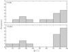 |
Fig. 1 Distributions of the acute angles between the radio polarization vectors and the jet axes of the 13 quasars from the VLBI compilation of Joshi et al. (2007) (top) and of the 15 quasars from the VLBA sample of Helmboldt et al. (2007) (bottom), with correction for SDSS J122127.04+441129.7. |
For our sample of 41 quasars3 in LQGs with m ≥ 10, we searched for jet axis information in the VLBI compilation of Joshi et al. (2007) and in the VLBA sample of Helmboldt et al. (2007). In these catalogues, we found 13 and 15 sources with jet position angle measurements, respectively4. For these objects, we computed the acute angle between the polarization vector and the jet axis. The distribution of these angles, shown in Fig. 1, demonstrates that even within our small sample the radio polarizations show a strong tendency to be perpendicular to the radio jets. Therefore, we safely conclude that in our sample the radio polarization vectors of the quasars trace the spin axes of the quasars and thus of their central SMBH. Any correlation found with the polarization vectors could then be interpreted in terms of the quasar spin axes.
3. Position angles of LQGs
To define the position angle of an LQG, we can proceed in two ways. We can consider a group of quasars as a cloud of points on the celestial sphere, or we can take the three-dimensional comoving positions of the sources into account. For either approach we determine the morphological position angle (MPA) of an LQG through the eigenvector of the inertia tensor corresponding to the major axis of the set of points.
For the two-dimensional approach, the quasar positions are projected onto the plane tangent to the celestial sphere. The orientation of the two-dimensional cloud of points is determined by computing its inertia tensor, assuming quasars to be unit point-like masses. The position angle of the eigenvector corresponding to the most elongated axis defines the morphological position angle of the large quasar group. We checked that this method returns position angles that are in excellent agreement (within 1 deg) with those obtained with an orthogonal regression (Isobe et al. 1990). The latter method was used in Hutsemékers et al. (2014) to define the position angles of the quasar groups.
For the second approach, the three-dimensional comoving positions of the quasars are used to determine the geometrical shape of an LQG by considering its tensor of inertia, assuming quasars to be unit point-like masses. A simple projection of the major axis of the fitted ellipsoid onto the plane orthogonal to the line of sight defines the position angle of the LQG.
As a result of the inclination of the system with respect to the line of sight, the MPAs determined by the two methods may differ. In our case, we found that they generally agree well. We show in Fig. 2 a comparison of the position angles of the LQGs that we obtained by the two- and three-dimensional procedures. While the two methods most often return MPAs that agree well, these quantities can be largely different owing to the apparent shape and the inclination of the system with respect to the line of sight. Because the two methods return similar results, we base our discussion on the three-dimensional approach, which is more physically motivated. In our calculation, we assume the same cosmological model as in Einasto et al. (2014), that is, a flat ΛCDM Universe with ΩM = 0.27.
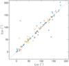 |
Fig. 2 Morphological position angles (in degrees) of the large quasar groups determined with the two-dimensional method (χ2D) as a function of those determined with the three-dimensional one (χ3D) for the 83 LQGs with m ≥ 5. Circles, squares, and triangles show LQGs with richness m< 10, 10 ≤ m< 20, and m ≥ 20, respectively. Some values of χ2D have been adjusted by 180° for clarity. |
For either approach, the morphological position angle of each large quasar group is derived at the centre of mass of the group. In general, a quasar for which we retrieved radio polarization measurement is angularly separated from the centre of mass of its hosting group. Hence, the acute angle between the two orientations (the polarization vector and the projected major axis) depends on the system of coordinates that is used. To overcome this coordinate dependence, we used parallel transport on the celestial sphere to move the projected eigenvector from the centre of mass of the group to the location of the quasar with polarization data. By introducing ψ for the polarization position angle of a quasar and χ for the (parallel-transported) position angle of the LQG to which it belongs, we compute the acute angle between the two orientations as 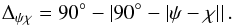 (1)The use of the parallel transport before evaluating the acute angle leads to coordinate-independent statistics. Both ψ and χ are defined in the range 0°−180° and are computed in the east-of-north convention.
4. Correlation between polarization and LQG position angles
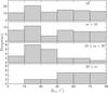 |
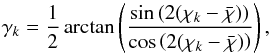
Fig. 3 Histogram of the distribution of Δψχ (in degree) for the 86 quasars with polarization–LQG position-angle measurements (top) and for the three sub-samples with richness m< 10, 10 ≤ m< 20, and m ≥ 20. |
In Fig. 3 (top) we show the distribution of Δψχ for the 86 quasars with polarization and LQG position-angle measurements. The distribution of the full sample (top) does not show any departure from uniformity. The probability given by a one-sample Kolmogorov-Smirnov (KS) test that the distribution is drawn from a uniform parent distribution is PKS = 88%. Since the alignment of optical polarization vectors with LQG orientations was found in very rich groups, and as the accuracy of the position angle of an LQG most likely depends on its richness, we divided our sample into three sub-samples with m< 10 (45 objects), 10 ≤ m< 20 (22 objects), and m ≥ 20 (19 objects). For the smallest LQGs (m< 10), the distribution of Δψχ does not show any departure from uniformity. The probability given by a one-sample KS test that the distribution is drawn from a uniform parent distribution is PKS = 54%. However, for the larger groups, a dichotomy is observed between the two sub-samples. The polarization vector of a quasar belonging to a very rich LQG (m ≥ 20) appears preferentially perpendicular to the projected major axis of the group (Δψχ> 45°), whereas the polarization vector of a quasar belonging to an LQG with medium richness (10 ≤ m< 20) seems to be preferentially parallel (Δψχ< 45°). A two-sample KS test tells us that the probability that the two parts of the sample with 10 ≤ m< 20 and m ≥ 20 have their distributions of Δψχ drawn from the same parent distribution is 0.05%.
For the 19 data points of the sub-sample of LQGs with m ≥ 20, 15 show Δψχ> 45°. The cumulative binomial probability of obtaining 15 or more data points with Δψχ> 45° by chance is Pbin = 0.96%. Of the 22 data points of the sub-sample of LQGs with 10 ≤ m< 20, 17 show Δψχ< 45°, which gives the cumulative binomial probability Pbin = 0.85%. These results indicate a correlation between the position angle of the major axis of an LQG and the radio polarization vector of its members in rich (m ≥ 10) quasar groups.
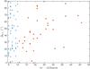 |
Fig. 4 Δψχ versus the richness m of the LQGs. For m ≤ 10 and m ≥ 11, symbols are triangles and filled squares, respectively. |
The dichotomy between the two sub-samples of LQGs with 10 ≤ m< 20 and m ≥ 20 is also illustrated in Fig. 4, where we plot the Δψχ of each quasar against the richness of its hosting LQG. Surprisingly, for m ≥ 11, we even see a possible linear correlation of Δψχ with the richness of the LQGs. A Spearman correlation test on the pairs Δψχ − m gives a rank-order correlation coefficient of 0.54 with a probability of obtaining this result by chance of 0.08%. For m< 10, there is no specific trend of Δψχ with the richness in agreement with the distribution seen in Fig. 3. To understand whether this lack of correlation for m< 10 is due to a larger uncertainty of the major axis position angles of the LQGs, as might naively be expected for the smallest groups, we estimated the confidence interval of the morphological position angle using the bootstrap method described in Appendix B. Keeping only MPAs for which the half-width confidence interval is below 20° (27 objects out of 45), the distribution of Δψχ remains uniform with PKS = 72%. The absence of alignments in LQGs with richness m< 10 is therefore likely to be real. On the other hand, the uncertainties, both on the position angles of the major axes of the LQGs and on the polarization position angles, cannot account for the correlations that we report. The introduction of poorly defined orientations in our analysis can only scramble an existing correlation. The same argument applies to the contamination of the polarization position angles by Galactic Faraday rotation, which is found to be negligible (see Appendix A).
In summary, our analysis shows that the quasars that belong to very rich (m ≥ 20) LQGs have polarization vectors preferentially perpendicular to the projected major axes of their hosting LQGs. The polarization vectors then become more often parallel to the LQG axes when m decreases before no correlation is observed for the smallest ones (m< 10).
5. Discussion
As discussed in Sect. 2, the radio polarization vector of a quasar is expected to be essentially perpendicular to the spin axis of its central engine. The correlation that we found between the polarization vectors and the major axes of the host LQGs might thus reflect an existing link between the spin axes of the quasars and the major axes of the host LQGs.
Our analysis independently supports the view that the spin axis of quasars that belong to very rich LQGs are preferentially parallel to the major axes of their hosting LQGs, as found in Hutsemékers et al. (2014). In addition, we found that the quasar-spin axes become preferentially perpendicular to the LQG’s major axes as the richness of the LQGs decreases, down to m ≥ 10.
Regardless of the richness dependence that we discuss below, our observation also suggests that the quasar spin axes have an intrinsic tendency to align themselves within their host LQGs. The observations of Jagannathan & Taylor (2014) that radio jets in the GRMT ELAIS N1 Deep Field align with each other over scales of 50−75 h-1 Mpc at redshift z ≳ 1 support our interpretation (Taylor & Jagannathan 2016).
As discussed in the introduction, the fact that the spin axes of black holes are found to align with their surrounding large-scale structures, which are assumed to be traced by LQGs, could be understood in the framework of the tidal torque theory if we accept that these predictions can be extrapolated to larger scales. However, and as far as we know, a richness dependence of the relative orientation is not a predicted feature of this theory. We therefore explore our data set to determine whether the richness dependence hides another dependence that could be more physically motivated.
For this exploratory analysis, we relied on our core sample of LQGs with m ≥ 10 and for which we have radio polarization measurements for at least one of their quasar member (Table C.1). For LQGs with m ≥ 10, the median of the diameters (the largest separation between two members in groups) is about 310 h-1 Mpc and the median separation of the closest pairs is about 45 h-1 Mpc.
5.1. Richness dependence and quasar intrinsic properties
N-body simulations have shown that the direction towards which the spin axes of dark-matter haloes preferentially point relative to the large-scale structure depends on their mass (Codis et al. 2015). As the masses of the SMBH and the host dark-matter halo are thought to be linked and as their spin axes might be aligned at high redshift (Dubois et al. 2014), we searched for a possible dependence of Δψχ with the black hole mass. Using the Spearman correlation test, we found that the SMBH masses (from Shen et al. 2011) do not show any correlation with Δψχ or with the richness of the host LQG. The same conclusion is reached if we consider other quasar properties reported in Shen et al. (2011), such as the radio-loudness, the width of the emission lines, or the redshift. There is thus apparently no hidden relation of Δψχ with quasar properties that could explain the richness dependence of Δψχ.
5.2. Richness dependence and LQG characteristics
In Sect. 3 we used the inertia tensors of the large quasar groups to assign their orientations in the three-dimensional comoving space. This resulted in fitting ellipsoids to the quasar systems. Here, we use the relative lengths of the principal axes of the ellipsoids to characterize their shapes. We found no correlation of Δψχ, or of the richness of the groups m, with geometrical characteristics of the LQGs such as their oblateness or departure from spherical or cylindrical symmetry.
A quantity that is related to the richness of an LQG and that could have a better physical meaning is its density. We can naively define the density of an LQG as ρ = m/V, where V is the comoving volume of its fitted ellipsoid. In our core sample of LQGs, there is a relation between the richness and the density: the richer a large quasar group, the lower its density. We then applied a Spearman correlation test to the pairs Δψχ − ρ, which resulted in rank-order correlation coefficient of −0.50 with a probability of obtaining this result by chance of 0.19%, if we consider all the LQGs with m ≥ 11 and at least one Δψχ measurement (the sub-sample studied in Sect. 4). SMBHs spin axes are thus parallel to the host LQG axis when the density of the latter is low and perpendicular when the density is high. The strength of this correlation is similar to the strength of the Δψχ − m correlation. The dependence between Δψχ and the richness m could then reflect a dependence between Δψχ and ρ, which might be easier to interpret. Codis et al. (2015) have shown that the spin axes of the dark-matter haloes of galaxies are preferentially parallel to their neighbouring filaments when the halo masses are low or, equivalently, when the density of their cosmic environment is low. When the density of the environment increases, the halo spin axis starts to avoid alignment with the filaments to finally point preferentially perpendicular to them. Our observations might thus support these predictions if we assume that, at least at redshift z ≥ 1.0, (i) a similar behaviour can be expected for the spin axes of the central SMBH of quasars; (ii) the density of an LQG reflects the density of the surrounding cosmic web; (iii) the LQGs can be used to trace the large-scale structures; and (iv) correlations that occur between the galaxy spin axes and filaments also occur at larger scales between quasar-spin axes and LQG major axes.
6. Conclusion
Studying the optical linear polarization of quasars that belong to two rich LQGs located at redshift z ~ 1.3, Hutsemékers et al. (2014) noted that the quasar polarization vectors do not point randomly with respect to the group structural axes. Using object spectra, they furthermore inferred that the spin axis of quasars, that is, the SMBH spin axes, are preferentially parallel to the major axes of the quasar groups. We here examined this result by considering the sample of LQGs published by Einasto et al. (2014), which is drawn from the SDSS DR7 quasar catalogue in the redshift range 1.0 ≤ z ≤ 1.8. We used the LQGs defined with a linking length of 70 h-1 Mpc. Because too few optical polarization data are available for the quasars that belong to the Einasto sample, we used radio polarization measurements from the JVAS/CLASS 8.4-GHz surveys (Jackson et al. 2007). This sample is claimed to be free of biases that might affect the polarization angles. Furthermore, the polarization vectors measured at 8.4 GHz have a strong tendency to be perpendicular to the spin axes of the SMBHs in the quasar cores. To compare the position angles of the quasar polarization vectors with the position angles of the systems to which the quasars belong, we studied the LQGs through their inertia tensors in the three-dimensional comoving space.
For rich quasar groups (m ≥ 20), we found that the spin axes of the SMBHs are preferentially parallel to the major axes of their host LQGs. This result adds weight to the previous finding by Hutsemékers et al. (2014) that in two LQGs the quasar spin axes (inferred from optical polarizations) align with the group axes. Combined with the initial discovery, our analysis indicates that the alignments of the SMBH spins axes with the LQG major axes do not depend on the quasar radio loudness.
Additionally, the use of a large sample of LQGs allowed us to probe the alignments for a wide variety of quasar systems. We unveiled a surprising correlation: the relative orientations of the spin axes of quasars with respect to the major axes of their host LQGs appear to depend on the richness of the latter, or equivalently on the density of objects. The spin axes of SMBHs appear preferentially parallel to the major axes of their host LQGs when the latter are very rich (or have a very low density), while the spin axes become preferentially perpendicular to the LQG major axes when the richness decreases to m ≥ 10 or, equivalently, when the quasar density increases to 1.5 × 10⁻⁵ (h-1 Mpc)-3. No correlation is observed below this richness or above this density. Possible interpretations were discussed in Sect. 5, but this intriguing feature needs to be confirmed.
In agreement with the view that the richest large quasar groups at high redshift most likely represent the progenitors of complexes or chains of superclusters (Einasto et al. 2014), the correlation that we found might be the high-redshift counterpart of the alignments at z ~ 0 of clusters of galaxies with the superclusters in which they are embedded (e.g. Einasto et al. 1980; West 1999).
The cut at m = 10 is justified below.
These two sub-samples are not independent. For the 9 objects in common, the jet position angles agree within ~20°, except for one source that shows an offset of about 72° (SDSS J122127.04+441129.7). After inspecting the VLBA maps (Helmboldt et al. 2007), we realized that the sign of the position angle of the VLBA jet needs to be changed for this object.
Acknowledgments
We thank D. Sluse for suggestions regarding the presentation of the work, M. Einasto for interesting discussions, and our referees for pointing out a mistake in the first version of the paper and for suggestions that improved the presentation of our results. D.H. is Senior Research Associate at the F.R.S.– FNRS. This work was supported by the Fonds de la Recherche Scientifique – FNRS under grant 4.4501.15. This research has made use of the NASA/IPAC Extragalactic Database (NED) which is operated by the Jet Propulsion Laboratory, California Institute of Technology, under contract with the National Aeronautics and Space Administration. This research has made use of NASA’s Astrophysics Data System.
References
- Aragón-Calvo, M. A., van de Weygaert, R., Jones, B. J. T., & van der Hulst, J. M. 2007, ApJ, 655, L5 [NASA ADS] [CrossRef] [Google Scholar]
- Catelan, P., & Theuns, T. 1996, MNRAS, 282, 436 [NASA ADS] [CrossRef] [Google Scholar]
- Clowes, R. G., Harris, K. A., Raghunathan, S., et al. 2013, MNRAS, 429, 2910 [NASA ADS] [CrossRef] [Google Scholar]
- Codis, S., Pichon, C., Devriendt, J., et al. 2012, MNRAS, 427, 3320 [NASA ADS] [CrossRef] [Google Scholar]
- Codis, S., Pichon, C., & Pogosyan, D. 2015, MNRAS, 452, 3369 [Google Scholar]
- Dubois, Y., Volonteri, M., & Silk, J. 2014, MNRAS, 440, 1590 [NASA ADS] [CrossRef] [Google Scholar]
- Einasto, J., Joeveer, M., & Saar, E. 1980, MNRAS, 193, 353 [NASA ADS] [CrossRef] [Google Scholar]
- Einasto, M., Tago, E., Lietzen, H., et al. 2014, A&A, 568, A46 [NASA ADS] [CrossRef] [EDP Sciences] [Google Scholar]
- Enea Romano, A., Cornejo, D., & Campusano, L. E. 2015, ArXiv e-prints [arXiv:1509.01879] [Google Scholar]
- Faltenbacher, A., Li, C., White, S. D. M., et al. 2009, RA&A, 9, 41 [Google Scholar]
- Fisher, N. I. 1993, Statistical Analysis of Circular Data [Google Scholar]
- Heavens, A., & Peacock, J. 1988, MNRAS, 232, 339 [NASA ADS] [CrossRef] [Google Scholar]
- Helmboldt, J. F., Taylor, G. B., Tremblay, S., et al. 2007, ApJ, 658, 203 [NASA ADS] [CrossRef] [Google Scholar]
- Hirata, C. M., & Seljak, U. 2004, Phys. Rev. D, 70, 063526 [NASA ADS] [CrossRef] [Google Scholar]
- Huchra, J. P., & Geller, M. J. 1982, ApJ, 257, 423 [NASA ADS] [CrossRef] [Google Scholar]
- Hutsemékers, D., Cabanac, R., Lamy, H., & Sluse, D. 2005, A&A, 441, 915 [NASA ADS] [CrossRef] [EDP Sciences] [Google Scholar]
- Hutsemékers, D., Braibant, L., Pelgrims, V., & Sluse, D. 2014, A&A, 572, A18 [NASA ADS] [CrossRef] [EDP Sciences] [Google Scholar]
- Isobe, T., Feigelson, E. D., Akritas, M. G., & Babu, G. J. 1990, ApJ, 364, 104 [NASA ADS] [CrossRef] [EDP Sciences] [Google Scholar]
- Jackson, N., Battye, R. A., Browne, I. W. A., et al. 2007, MNRAS, 376, 371 [NASA ADS] [CrossRef] [Google Scholar]
- Jagannathan, P., & Taylor, R. 2014, in Alignments of Radio Sources in the GMRT ELAIS N1 Deep Field, Am. Astron. Soc. Meet. Abstr., 223, 150 [Google Scholar]
- Joachimi, B., Cacciato, M., Kitching, T. D., et al. 2015, Space Sci. Rev., 193, 1 [NASA ADS] [CrossRef] [Google Scholar]
- Jones, B. J. T., van de Weygaert, R., & Aragón-Calvo, M. A. 2010, MNRAS, 408, 897 [NASA ADS] [CrossRef] [Google Scholar]
- Joshi, S. A., Battye, R. A., Browne, I. W. A., et al. 2007, MNRAS, 380, 162 [NASA ADS] [CrossRef] [Google Scholar]
- Kiessling, A., Cacciato, M., Joachimi, B., et al. 2015, Space Sci. Rev., 193, 67 [NASA ADS] [CrossRef] [Google Scholar]
- Kirk, D., Brown, M. L., Hoekstra, H., et al. 2015, Space Sci. Rev., 193, 139 [NASA ADS] [CrossRef] [Google Scholar]
- Lee, J., & Pen, U.-L. 2000, ApJ, 532, L5 [NASA ADS] [CrossRef] [PubMed] [Google Scholar]
- Lee, J., & Pen, U.-L. 2001, ApJ, 555, 106 [NASA ADS] [CrossRef] [Google Scholar]
- Li, C., Jing, Y. P., Faltenbacher, A., & Wang, J. 2013, ApJ, 770, L12 [NASA ADS] [CrossRef] [Google Scholar]
- McKinney, J. C., Tchekhovskoy, A., & Blandford, R. D. 2013, Science, 339, 49 [NASA ADS] [CrossRef] [PubMed] [Google Scholar]
- Nadathur, S. 2013, MNRAS, 434, 398 [NASA ADS] [CrossRef] [Google Scholar]
- Oppermann, N., Junklewitz, H., Greiner, M., et al. 2015, A&A, 575, A118 [NASA ADS] [CrossRef] [EDP Sciences] [Google Scholar]
- Park, C., Song, H., Einasto, M., Lietzen, H., & Heinamaki, P. 2015, J. Kor. Astron. Soc., 48, 75 [NASA ADS] [CrossRef] [Google Scholar]
- Pelgrims, V., & Hutsemékers, D. 2015, MNRAS, 450, 4161 [NASA ADS] [CrossRef] [Google Scholar]
- Pen, U.-L., Lee, J., & Seljak, U. 2000, ApJ, 543, L107 [NASA ADS] [CrossRef] [Google Scholar]
- Pollack, L. K., Taylor, G. B., & Zavala, R. T. 2003, ApJ, 589, 733 [NASA ADS] [CrossRef] [Google Scholar]
- Rusk, R., & Seaquist, E. R. 1985, ApJ, 90, 30 [Google Scholar]
- Saikia, D. J., & Salter, C. J. 1988, ARA&A, 26, 93 [NASA ADS] [CrossRef] [Google Scholar]
- Shen, Y., Richards, G. T., Strauss, M. A., et al. 2011, ApJS, 194, 45 [NASA ADS] [CrossRef] [Google Scholar]
- Taylor, A. R., & Jagannathan, P. 2016, MNRAS, 459, L36 [NASA ADS] [CrossRef] [Google Scholar]
- Tempel, E., & Libeskind, N. I. 2013, ApJ, 775, L42 [NASA ADS] [CrossRef] [Google Scholar]
- Wardle, J. F. C. 2013, in Eur. Phys. J. Web Conf., 61, 6001 [Google Scholar]
- West, M. J. 1994, MNRAS, 268, 79 [NASA ADS] [CrossRef] [Google Scholar]
- West, M. J. 1999, in The Most Distant Radio Galaxies, eds. H. J. A. Röttgering, P. N. Best, & M. D. Lehnert, 365 [Google Scholar]
- White, S. D. M. 1984, ApJ, 286, 38 [NASA ADS] [CrossRef] [Google Scholar]
- Zhang, Y., Yang, X., Wang, H., et al. 2013, ApJ, 779, 160 [NASA ADS] [CrossRef] [Google Scholar]
Appendix A: Contamination by Galactic Faraday rotation
Although Jackson et al. (2007) and Joshi et al. (2007) stated that the Faraday rotation of our Galaxy can be neglected for quasars observed at 8.4 GHz, it is important to verify that this contamination is indeed negligible for our sample.
We used the all-sky Galactic Faraday map produced by Oppermann et al. (2015) to verify that the Galactic Faraday rotation can be neglected in our analysis. From their map of rotation measures, we extracted the whole sky window covered by the Einasto sample. For the entire window, the distribution of the Faraday rotation angles at 8.4 GHz that is due to the Galactic magnetic field has a mean at 0.6° and a standard deviation of about 1°. For the source locations of our sample with polarization measurements (the 185 JVAS/CLASS sources), the contamination is even lower with a mean of 0.5° and a standard deviation of 0.6°. We conclude that the Galactic Faraday rotation can be neglected because the rotation angles are within the error bars of the polarization data.
Appendix B: Position angles and their uncertainties
To quantify the uncertainties of the morphological position angles (MPA) that characterize the LQGs, we used the bootstrap method. This procedure allows properly accounting for the circular nature of the data (Fisher 1993). For a given LQG of richness m, we produced Nsim bootstrap LQGs with the same number of members, allowing replicates. The position angle of each bootstrap LQG is determined through the inertia tensor procedure used for real groups. As this procedure is not properly defined for groups resulting in only one point, we took care in the generation of LQGs to avoid bootstrap samples consisting of m replications of the same source. The probability that such a configuration occurs is m1 − m. Hence, the rejection procedure can only affect poor LQGs. We note that even for those poor LQGs, the effect of theses configurations on the evaluation of the confidence interval is negligible (≪1°). For a given group of quasars, we therefore collected a corresponding distribution of Nsim estimates of the morphological position angle. From this distribution, we evaluated the mean and its corresponding confidence interval. For a distribution of axial-circular quantities χk such as the position angle of the LQG major axes, the mean is computed as (Fisher 1993) 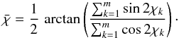 (B.1)Since there is no proper definition of the standard deviation for axial-circular data, we evaluated the confidence interval of the unknown mean at the 100 (1−α)% level as follows (Fisher 1993). We defined
 (B.2)
(B.2)
where k = 1,...,Nsim. The γk were defined in the range [− 90°, 90°]. Then we sorted the γk in increasing order to obtain γ(1) ≤ ... ≤ γ(Nsim). If l is the integer part of  and u = Nsim − l, the confidence interval for
  is
is ![Mathematical equation: \hbox{$\left[ \bar{\chi} + \gamma_{(l+1)}, \, \bar{\chi} + \gamma_{(u)} \right]$}](/articles/aa/full_html/2016/06/aa26979-15/aa26979-15-eq117.png) . We chose to compute the confidence interval of at the 68% confidence level. We defined the half-width of the confidence interval as HWCI = (γ(u) − γ(l + 1))/2.
. We chose to compute the confidence interval of at the 68% confidence level. We defined the half-width of the confidence interval as HWCI = (γ(u) − γ(l + 1))/2.
Using the bootstrap method with 10 000 simulations, we evaluated the HWCIs for the 83 (independent) LQGs of our sample. The distribution of HWCI corresponding to the three-dimensional evaluation of the morphological position angles is shown in Fig. B.1 for different cuts in richness and is compared to those obtained from the two-dimensional procedure.
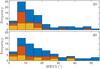 |
Fig. B.1 Histograms of the half-width confidence interval (HWCI) for the MPA values obtained for the 83 independent LQGs with the two- (top) and three-dimensional (bottom) approaches (see Sect. 3). The HWCIs are evaluated using the bootstrap method as explained in the text. Histograms are for m ≥ 5 (blue), m ≥ 10 (orange), and m ≥ 20 (yellow). |
In general, the HWCIs are lower when the two-dimensional procedure is chosen to estimate the MPAs. The highest values of the HWCIs (≥20°) can in general mostly be attributed to poor LQGs with m< 10, as naively expected.
Appendix C: Data sample
Table C.1 summarizes the data for the 41 quasars hosted in LQGs with m ≥ 10. For each quasar for which we collected polarization measurements, we list the SDSS name, its redshift, the position angle of its polarization vector (ψ), the identification index of the LQG to which it belongs (following the numbering of Einasto et al. 2014), the richness of the group, and the position angle of the projected major axis (χ3D). In Figs. C.1 and C.2 we show the projection on the sky of the medium and high richness parts of the LQG sample with 10 ≤ m< 20 and m ≥ 20, respectively. We highlighted those LQGs for which we retrieved the radio polarization for at least one member and show the orientations of the projected major axes along with the polarization vectors of the quasars.
Data for the 41 quasars with Δψχ measurements and belonging to rich (m ≥ 10) LQGs.
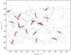 |
Fig. C.1 Projection on the sky, in SDSS coordinates, of the LQGs with a richness in the range 10–19 (clouds of grey dots). The LQGs containing at least one quasar with polarization measurements (circled in red) are highlighted in blue. The black lines trace the orientation of the projected major axes of the groups (here at the centres of masses). The red lines give the orientations of the polarization vectors. All lines are of equal lengths for clarity. The polarization vectors are preferentially parallel to the projected major axes of the groups. |
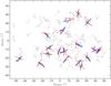 |
Fig. C.2 Same as Fig. C.1, but for the LQGs with at least 20 members. The polarization vectors are preferentially perpendicular to the projected major axes of the groups. |
All Tables
Data for the 41 quasars with Δψχ measurements and belonging to rich (m ≥ 10) LQGs.
All Figures
|
Fig. 1 Distributions of the acute angles between the radio polarization vectors and the jet axes of the 13 quasars from the VLBI compilation of Joshi et al. (2007) (top) and of the 15 quasars from the VLBA sample of Helmboldt et al. (2007) (bottom), with correction for SDSS J122127.04+441129.7. |
| In the text | |
|
Fig. 2 Morphological position angles (in degrees) of the large quasar groups determined with the two-dimensional method (χ2D) as a function of those determined with the three-dimensional one (χ3D) for the 83 LQGs with m ≥ 5. Circles, squares, and triangles show LQGs with richness m< 10, 10 ≤ m< 20, and m ≥ 20, respectively. Some values of χ2D have been adjusted by 180° for clarity. |
| In the text | |
|
Fig. 3 Histogram of the distribution of Δψχ (in degree) for the 86 quasars with polarization–LQG position-angle measurements (top) and for the three sub-samples with richness m< 10, 10 ≤ m< 20, and m ≥ 20. |
| In the text | |
|
Fig. 4 Δψχ versus the richness m of the LQGs. For m ≤ 10 and m ≥ 11, symbols are triangles and filled squares, respectively. |
| In the text | |
|
Fig. B.1 Histograms of the half-width confidence interval (HWCI) for the MPA values obtained for the 83 independent LQGs with the two- (top) and three-dimensional (bottom) approaches (see Sect. 3). The HWCIs are evaluated using the bootstrap method as explained in the text. Histograms are for m ≥ 5 (blue), m ≥ 10 (orange), and m ≥ 20 (yellow). |
| In the text | |
|
Fig. C.1 Projection on the sky, in SDSS coordinates, of the LQGs with a richness in the range 10–19 (clouds of grey dots). The LQGs containing at least one quasar with polarization measurements (circled in red) are highlighted in blue. The black lines trace the orientation of the projected major axes of the groups (here at the centres of masses). The red lines give the orientations of the polarization vectors. All lines are of equal lengths for clarity. The polarization vectors are preferentially parallel to the projected major axes of the groups. |
| In the text | |
|
Fig. C.2 Same as Fig. C.1, but for the LQGs with at least 20 members. The polarization vectors are preferentially perpendicular to the projected major axes of the groups. |
| In the text | |
Current usage metrics show cumulative count of Article Views (full-text article views including HTML views, PDF and ePub downloads, according to the available data) and Abstracts Views on Vision4Press platform.
Data correspond to usage on the plateform after 2015. The current usage metrics is available 48-96 hours after online publication and is updated daily on week days.
Initial download of the metrics may take a while.