| Issue |
A&A
Volume 589, May 2016
|
|
|---|---|---|
| Article Number | A102 | |
| Number of page(s) | 11 | |
| Section | Astrophysical processes | |
| DOI | https://doi.org/10.1051/0004-6361/201628341 | |
| Published online | 20 April 2016 | |
Clumpy wind accretion in supergiant neutron star high mass X-ray binaries
1 ISDC Data Centre for Astrophysics, Chemin d’Ecogia 16, 1290 Versoix, Switzerland
e-mail: This email address is being protected from spambots. You need JavaScript enabled to view it.
2 Institut für Physik und Astronomie, Universität Potsdam, Karl-Liebknecht-Strasse 24/25, 14476 Potsdam, Germany
3 International Space Science Institute (ISSI), Hallerstrasse 6, 3012 Bern, Switzerland
4 International Space Science Institute in Beijing, No. 1 Nan Er Tiao, Zhong Guan Cun, 100190 Beijing, PR China
Received: 19 February 2016
Accepted: 16 March 2016
Abstract
The accretion of the stellar wind material by a compact object represents the main mechanism powering the X-ray emission in classical supergiant high mass X-ray binaries and supergiant fast X-ray transients. In this work we present the first attempt to simulate the accretion process of a fast and dense massive star wind onto a neutron star, taking into account the effects of the centrifugal and magnetic inhibition of accretion (“gating”) due to the spin and magnetic field of the compact object. We made use of a radiative hydrodynamical code to model the nonstationary radiatively driven wind of an O-B supergiant star and then place a neutron star characterized by a fixed magnetic field and spin period at a certain distance from the massive companion. Our calculations follow, as a function of time (on a total timescale of several hours), the transitions of the system through all different accretion regimes that are triggered by the intrinsic variations in the density and velocity of the nonstationary wind. The X-ray luminosity released by the system is computed at each time step by taking into account the relevant physical processes occurring in the different accretion regimes. Synthetic lightcurves are derived and qualitatively compared with those observed from classical supergiant high mass X-ray binaries and supergiant fast X-ray transients. Although a number of simplifications are assumed in these calculations, we show that taking into account the effects of the centrifugal and magnetic inhibition of accretion significantly reduces the average X-ray luminosity expected for any neutron star wind-fed binary. The present model calculations suggest that long spin periods and stronger magnetic fields are favored in order to reproduce the peculiar behavior of supergiant fast X-ray transients in the X-ray domain.
Key words: stars: neutron / X-rays: binaries / supergiants
© ESO, 2016
1. Introduction
Most of the supergiant high mass X-ray binaries (SGXBs), including the supergiant fast X-ray transients (SFXTs), host a neutron star (NS) accreting from the fast, dense wind of a massive O-B supergiant companion. The accretion of the stellar wind material onto the compact object powers a conspicuous X-ray emission (see Walter et al. 2015, for a recent review).
The so-called classical SGXBs are typically characterized by a relatively constant average X-ray luminosity. Depending mostly on the orbital separation between the NS and the companion, this luminosity can range from 1034 erg s-1 to 1037 erg s-1 and displays a short-term variability achieving a dynamic range in the X-ray luminosity of 10−100 over timescales of a hundred to a thousand seconds. The SFXTs are known instead to display a much more extreme behavior in the X-ray domain. These sources remain in quiescence (LX ~ 1032−1033 erg s-1) for most of the time and only sporadically undergo short, bright outbursts, reaching a luminosity comparable to that of the classical systems (LX ~ 1036−1037 erg s-1). The dynamical range of the SFXT X-ray luminosity can thus achieve values as large as ΔLX ~ 105−106 (Romano et al. 2015). The outbursts of these sources last for a few hours at the most, and thus their activity duty cycle is estimated to be typically of a few percent (Lutovinov et al. 2013; Romano et al. 2011, 2014a; Paizis & Sidoli 2014; Bozzo et al. 2015). In virtually all SFXTs it has also been observed that X-ray flares reaching a luminosity of 1−10% of that of the brightest outbursts can occur at any time, displaying timing and spectral properties similar to those of the more luminous events (see, e.g., Sidoli et al. 2008; Bozzo et al. 2010; Bodaghee et al. 2010; Romano et al. 2013, 2014b).
The spectroscopic properties of the SFXT X-ray emission is typical of wind accreting NS systems and can be usually described by using a power-law model with a cut-off around 10−30 keV (see, e.g., Romano et al. 2008; Sidoli et al. 2009; Romano 2015). Soft thermal components have been detected in the X-ray spectra of the SFXTs both during outbursts and quiescence. In the first case, these components are mostly ascribed to hot spots on the NS surface, while in quiescence the thermal emission could be more easily explained as being produced within the wind of the supergiant companion (Bozzo et al. 2010; Sidoli et al. 2010).
The winds of OB supergiants are known to produce a relatively bright X-ray emission that could reach values of 1034 erg s-1 in the most extreme cases. The origin of these X-rays is still highly debated, but one of the most credited hypotheses is that they are produced by the collision of “clumps” in the stellar wind, i.e., structures characterized by a higher density and a different velocity than the surrounding intra-clump medium (see, e.g., Feldmeier 1995; Oskinova et al. 2006, and references therein). One of the stellar wind models developed to study the formation of clumps and the release of X-ray radiation from their collisions was presented by Feldmeier et al. (1997b). This radiatively nonstationary wind model allows us to carry out a hydrodynamic investigation of the wind formation and evolution from the first principles, together with the computation of the thermal structure of the wind and the energy distribution of the emitted radiation. The model uses a 1D approach and thus the clumps can grow significantly in size and density owing to the lack of the other two spatial dimensions that would allow us to observe the lateral break-up of these structures as a consequence of the Rayleigh-Taylor or thin-shell instability (Dessart & Owocki 2003, 2005). Multidimensional simulations (mostly 2D and pseudo 3D), however, have so far been unable to account for the thermal structure of the wind and thus they have not made any clear prediction on the intensity of the produced X-ray radiation to be compared with observations of isolated OB supergiants and massive stars in SGXBs (see, e.g., Puls et al. 2008). More recent findings seem to suggest that clumps might likely be limited to a density ratio of ~10 compared to the surrounding medium and a lateral extent on the order of 10% of the supergiant star radius (see, e.g., Šurlan et al. 2013, and references therein).
The possibility of having massive and dense structures in the winds of supergiant stars, as predicted by the 1D approach of stellar wind models mentioned above, stimulated the idea that the SFXTs might have been a subclass of SGXBs hosting massive stars with extreme clumpy winds (in’t Zand 2005; Negueruela et al. 2006, 2007; Walter & Zurita Heras 2007; Bozzo et al. 2011). In this scenario the accretion of a massive clump onto the NS would produce short, bright X-ray outbursts as the duration of the event is related to the lateral size of the clump while the total luminosity is directly proportional to its mass. Less luminous flares can be explained by invoking a reasonable distribution in mass and size of the clumps (in’t Zand 2005; Walter & Zurita Heras 2007). The quiescent emission of the SFXT can be interpreted in this scenario by assuming that in this case the NS is accreting through the much more rarefied intra-clump medium, whose particularly low density can only provide a feeble mass accretion rate onto the compact object.
The first attempt to combine nonstationary stellar wind codes with calculations on the expected accretion luminosity produced by a NS located inside the wind was presented by Oskinova et al. (2012b). These authors assumed the simplest accreting scenario in which all the stellar wind material gravitationally captured by the NS is accreted onto the compact object. Their calculations showed that the extremely clumpy wind produced by the 1D code gives rise to a large X-ray variability reaching a dynamic range of 106−107. Even though this is compatible with the dynamic range displayed by the SFXTs, the overall behavior observed in the simulations of Oskinova et al. (2012b) did not resemble that typically observed from the sources in this class. In particular, the model failed to reproduce the SFXT low duty cycle as it predicted that bright outbursts could repeat at any time without the presence of extended periods of quiescence.
As discussed by Bozzo et al. (2015), it is likely that extremely clumpy winds are not enough to explain the complex phenomenology of the SFXTs; some additional mechanism is needed to halt the accretion onto the NS for a large fraction of time and to reproduce the low duty cycles of these systems (see also Romano et al. 2014a; Sidoli et al. 2016). Bozzo et al. (2008, hereafter B08) proposed that the inhibition of accretion could occur in the SFXTs owing to a peculiarly intense magnetic field and slow rotation of the compact object1. The NS rotation and magnetic field were indeed shown to give rise to a centrifugal and magnetic gate that can inhibit accretion through either the onset of a propeller effect (Illarionov & Sunyaev 1975; Grebenev & Sunyaev 2007) or by preventing the gravitational focusing of the wind material toward the NS.
In this paper we take a step forward from the simulations presented by Oskinova et al. (2012b) and show how the magnetic and centrifugal gating mechanisms proposed by B08 would work in presence of a nonstationary clumpy stellar wind. Our aim is to provide a refined calculation of the accretion luminosity that arises in wind accreting systems and to investigate on timescales spanning several hours whether the centrifugal and magnetic gating mechanisms can help to reproduce the characteristic behavior of the SFXTs in the X-ray domain. In Sect. 2 we summarize the main properties of the 1D clumpy wind model already used by Oskinova et al. (2012b), and provide a brief description of the gating accretion models of B08 in Sect. 3. The results obtained by taking into account the gating mechanisms during the accretion of the clumpy stellar wind material onto a NS are described in Sect. 4. We provide our discussion and conclusions in Sect. 5.
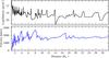 |
Fig. 1 Snapshot at a fixed time of the density stratification (upper panel) and velocity field (lower panel) of the stellar wind in a O9.5 supergiant star, as predicted by time-dependent hydrodynamic simulations described in Sect. 2. The upper panel shows that the wind density can change by several orders of magnitude owing to the presence of clumps. The corresponding strong wind velocity jumps are visible in the lower panel. |
2. Clumpy winds
To simulate the wind of the OB supergiant star hosted in a SGXB or SFXT we use the results from hydrodynamic simulations that derive the dynamics and the thermal structure of a line driven stellar wind from the first principles (see Feldmeier 1995; Feldmeier et al. 1997b,a, for more details). This is the same model adopted by Oskinova et al. (2012a) that predicts highly structured and nonstationary stellar winds with large density and velocity gradients. In the model, clumps are produced as a consequence of the line-driven instability (LDI; Lucy & White 1980). The unstable growth of the LDI is triggered by seed perturbations at the base of the wind in the form of turbulent variations of velocity and density at a level of roughly one-third of the sound speed. These perturbations have a coherence time of 1.4 h, which is close to the acoustic cutoff period of the model star. The assumed stellar parameters are typical of a late O-type supergiant, but it has been shown that the predicted stellar wind dynamic structures of the model are not sensitive to reasonable variations in the input stellar parameters.
Figure 1 shows a snapshot at a fixed time of the wind structure produced by the model as a function of the distance from the massive star. The model predicts a quasi-continuous hierarchy of density and velocity structures in the wind where dense shells are formed relatively close to the star during the first stage of unstable growth of the LDI. The dense shells have a rather small radial extent, low electron temperatures (Te ~ 10 kK), and contain the bulk of the wind mass. The colloquial term “wind clumps” refers to these dense shells. The space between the shells is filled with low density gas, which is usually termed “intra-clump” medium.
In addition to the dense cool shells and the tenuous intra-clump medium, there is a third type of structure. These structures can be described as small “clouds” that are accelerated by the stellar radiation field and eventually collide with the next-outer dense shell. The collisions between clouds and shell are the mechanism through which the model produces the X-ray emission with properties close to those observed from early-type stars at high energies (Feldmeier et al. 1997b,a; Oskinova et al. 2006).
In these time-dependent hydrodynamic simulations, the time-averaged velocity field of the stellar wind follows the so-called β-law, vw(r) = v∞(1−1 /r)β, where v∞ is the wind terminal speed and r is the distance from the center of the massive star in units of the stellar radius. This velocity field is naturally obtained as an outcome of the hydrodynamical model. Strong velocity jumps are produced in the model with negative gradients across the shells. Even relatively close to the star, the wind velocity can change by hundreds of km s-1 within a few hours. The model includes the incremental growth of the optical depth owing to multiple resonances in a nonmonotonic velocity field, and is able to resolve the cooling zones behind strong shocks. This provides a complete and detailed hydrodynamic description of the stellar wind (radiation, temperature, density, and velocity), which is currently possible only in similar 1D models.
3. Gated accretion models
In this section we review the gating accretion model presented by B08 that illustrates all the different accretion regimes that a NS hosted in a SGXB or an SFXT can experience (see also Lipunov 1987; Lipunov et al. 1992, for previous treatments of the wind accretion regimes). At odds with the more simplified approach of the Bondi-Hoyle accretion (see Appendix A) adopted by Oskinova et al. (2012b), the gating accretion model takes into account the effect produced on the accretion flow by the NS spin and magnetic field. The characteristics and the main physical processes dominating the X-ray emission in each accretion regime are briefly summarized below. We refer the reader to the original paper of B08 for further details on the model and on all involved assumptions. We define:
-
The accretion radius, Ra, as the distance from the NS at which the inflowing stellar wind material is gravitationally focused toward the compact object,
 (1)where vrel is the relative velocity of the NS with respect to the stellar wind and v8 is the stellar wind velocity in units of 1000 km s-1. We assume here for simplicity that the orbital velocity of the NS is negligible compared to vw (as was done in B08).
 -
The magnetospheric radius, RM, as the distance at which the pressure of the NS magnetic field balances the ram pressure of the inflowing matter. If the magnetospheric radius is larger than the accretion radius Ra, the former can be calculated as
 (2)Here2μ33 = μ/ 1033 G cm3 is the NS dipolar magnetic field and ρ-12 = ρw/(10-12 g cm-3) is the density of the stellar wind close to the compact object.
 -
The corotation radius, Rco, as the distance at which the velocity of the NS spin rotation equals the local Keplerian angular velocity, i.e.,
 (3)where Ps3 is the NS spin period in units of 103 s.
We additionally define the orbital separation between the NS and the supergiant companion as a = 4.2 × 10¹²a10d cm, where  , P10d is the binary orbital period in units of 10 days, and M30 is the total mass of the system (NS + supergiant companion) in units of 30 M⊙. We assume in all cases a circular orbit, as was originally done in B08. We note that all radii defined above are much smaller than the supergiant radius and the radial extent of the clump structures mentioned in Sect. 2, thus justifying the use of the 1D model for these systems.
The conditions under which the different accretion regimes can occur depend mostly on the relative position of the accretion radius, the corotational radius, and the mangetospheric radius. As shown by the equations above, the corotation radius is only a function of the NS spin period and can thus be considered constant once Pspin is fixed3. The accretion radius and the magnetospheric radius are, instead, strongly dependent on the properties of the stellar wind and can thus change significantly if the properties of the medium surrounding the compact object are altered, e.g., by the presence of a clump. We have to distinguish a number of different possibilities, as illustrated in the following sections.
3.1. RM1 > Ra
We begin by considering the case in which the magnetospheric radius is larger than the accretion radius. Before entering the details of the X-ray emission released in this regime we first have to distinguish between the two cases below:
-
RM1 ≥ Rco. If RM1>Ra and RM1>Rco, we are in the so-called super-Keplerian magnetic inhibition regime. In this case, both the magnetic and the centrifugal gates are closed and inhibit the accretion onto the NS. In particular, the magnetic gate prevents matter from being gravitationally focused toward the NS and the centrifugal gate propels the material away along the magnetospheric boundary of the compact object. The X-ray luminosity of the system is dominated in this case by the energy released in the shocks occurring close the magnetospheric boundary (RM = RM1) and by friction between the rotating NS magnetosphere and the surrounding material. We thus have
 (4)where
  (5)and
  (6)
(6) -
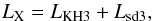
RM1<Rco. In this case only the magnetic gate is closed and we are in the sub-Keplerian magnetic inhibition of accretion. Matter is still not gravitationally focused toward the compact object, but since the propeller effect is not effective, the material passing along the magnetospheric boundary of the compact object is not pushed away and can accrete mainly through the Kelvin-Helmholtz instability (hereafter KHI). As shown by B08, the total X-ray luminosity is given in this case by
 (7)where
  (8)and
  (9)We assume for the present work the reasonable value of 0.5 for the ratio between the wind density material inside (ρi) and outside (ρe) the compact object mangetospheric boundary. We also use a standard value for the parameter of the KHI efficiency ηKH = 0.1 (B08). Higher values of this quantity will only slightly increase the X-ray luminosity in the sub-Keplerian magnetic inhibition regime, but do not qualitatively change the results discussed in Sect. 4.
3.2. R M1 < R a
When the magnetospheric radius RM1<Ra, the magnetic gate is open and the inflowing material from the stellar wind can be gravitationally focused toward the compact object, filling the space between Ra and the magnetospheric radius. This material redistributes itself into an approximately spherical configuration resembling an atmosphere whose shape and properties are determined by the interaction with the rotating NS magnetosphere at the magnetospheric boundary.
The equation defining the magnetospheric radius changes as the pressure of the material is now computed assuming a hydrostatic equilibrium and we have RM = RM2, where  (10)Before computing the X-ray luminosity released in this case, we have to distinguish between the different cases below:
-
RM2 > Rco: in this case the centrifugal gate is closed and the rapid rotation of the NS propels the inflowing material away after it has been gravitationally focused. We are thus in the so-called supersonic propeller regime. Matter entered within the accretion radius cannot accrete onto the NS and the main contribution to the X-ray luminosity of the system is due to the friction of the material around the NS and the compact object magnetosphere:
 (11)In the above equation cs(RM) = vff(RM) = (2GMNS/RM)1/2 is the sound velocity in the shell of material surrounding the NS.
 -
RM2 < Rco: if RM2 is no longer larger than the corotation radius, then both the magnetic and centrifugal gates are open and the inflowing stellar wind material can begin penetrating the NS magnetosphere and accreting onto the compact object. In this situation, the rotational velocity of the NS magnetosphere is subsonic and the magnetospheric radius has to be calculated according to the following equation:
 (12)Accretion at full regime, however, can take place only when there is a sufficiently high density outside RM3, such that the inflowing wind material can cool down rapidly and the magneto-hydrodynamic instabilities at the NS magnetospheric boundary reach the highest efficiency in transporting material inside the NS magnetosphere. The critical density above which accretion occurs at full regime (i.e., comparable with the accretion rate in the Bondi-Hoyle approximation) is given by
  (13)where RM10 = RM3/1010. We thus still have to distinguish between two additional cases:
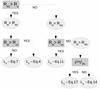
Fig. 2 Schematic flow of the conditions that are considered within the clumpy wind code to establish which is the relevant accretion regime for the system at each time step and how the total X-ray luminosity should be calculated.
-
If ρ-12 < ρlim-12, then accretion does not achieve the highest efficiency and the system enters the subsonic propeller regime. It can be shown that the main contributions to the total released X-ray luminosity is provided by the partly limited accretion allowed by the KHI and the friction between the material surrounding the NS and its magnetosphere,
 (14)where
 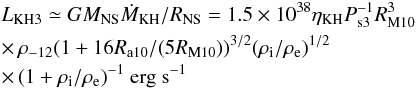 (15)and
  (16)
(16) -
If ρ-12 ≥ ρlim-12, then all conditions are satisfied for accretion at full regime to take place. The system thus achieves the highest X-ray luminosity and enters the so-called direct accretion regime. In this case the mass accretion rate is comparable to the Bondi-Hoyle approximation and we have
 (17)
(17)
-
All equations in this section have been re-adapted from B08 to be used within the clumpy wind code described in Sect. 2. This code provides the value of the wind velocity v8 and the density ρ-12 as a function of time at the NS location (which is a fixed parameter). These values are first used to determine which accretion regime the system is experiencing at a certain time and then to estimate the corresponding X-ray luminosity. A schematic version of the flow of conditions that lead the code to establish the relevant accretion regime of the system and compute the X-ray luminosity at each time step is shown in Fig. 2.
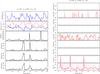 |
Fig. 3 Results of the simulations of the accretion onto a NS using the nonstationary wind model introduced in Sect. 2 and taking into account the gating accretion mechanisms described in Sect. 3. The system parameters adopted in the simulation are shown above each figure (a separation of 2.5 R∗ corresponds to an orbital period of 9.1 days). Left figure: wind velocity and density as a function of time, and all relevant radii to be determined in the gating accretion model. In the density panel we also show the value of the critical density in Eq. (13) (red dashed line). Right figure (all panels): different contributions to the total X-ray luminosity of the system, which is given in the bottom panel, together with the corresponding X-ray luminosity that would be achieved by assuming the simplest Bondi-Hoyle scenario (magenta solid line; see Appendix A). Empty regions in each panel represent time intervals in which the corresponding quantity is not calculated because the source is not in that specific accretion regime (or is out of scale and thus negligible for the overall luminosity budget; see Sect. 4 for details). |
4. Results
We present in this section the results obtained by simulating the accretion of the clumpy wind model in Sect. 2 onto a strongly magnetized rotating NS. The main parameter to be fixed for the clumpy wind model is the distance between the compact object and the massive companion, i.e., the orbital separation. As we discussed in Sect. 2, the properties of the stellar wind change at different distances from the massive stars, thus affecting the physical properties of the accretion flow that approaches the NS as a function of time. We discuss below the two cases in which the NS is located at a = 2.5R∗ and 5R∗ from the massive companion (here R∗ is the supergiant radius). Because we considered in all cases a supergiant star with a mass of 34 M⊙ and a radius of 24 R⊙, the above separations correspond to a NS orbital period of 9.1 and 25.6 days, respectively (a circular orbit is assumed in all cases as we cannot simulate the effect of a non-negligible eccentricity in the present set-up). In order to probe different combinations of the accretion regimes, we also considered different cases for the NS magnetic field and spin period. In particular, we report here on three cases: (i) Ps3 = 1 and μ33 = 0.1; (ii) Ps3 = 1 and μ33 = 0.001; and (iii) Ps3 = 0.01 and μ33 = 0.001. The first of these possibilities is more representative of the accretion onto slowly rotating “magnetars”, i.e., NSs endowed with particularly strong magnetic fields. The second and the third cases are more representative of a normal pulsar in a SGXBs, endowed with a standard magnetic field of 1012 G and a longer or shorter spin period.
4.1. Orbital period 9.1 days
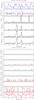 |
Fig. 4 Same as Fig. 3 but for a NS spin period of 1000 s. The magnetic field strength was not changed. |
We show the outcomes of the combination of the clumpy wind code with the different accretion regimes for an orbital period of 9.1 days in Figs. 3−5.
The first of these figures shows the fastest spin period (Ps3 = 0.01) and lowest magnetic field (μ33 = 0.001) case considered in this paper. The top two panels of Fig. 3 (left) show the velocity and density evolution as a function of time computed within the clumpy wind model in Sect. 2. In the density panel, we also overplot the value of the critical density obtained from Eq. (13). The other panels show from bottom to top the magnetospheric radii (RM1, RM2, and RM3) applicable to the different accretion regimes and measured in units of the corotation radius Rco. We also display in the same units the accretion radius, Ra. Depending on the relative position of these radii, it can be understood how changes in the local environment surrounding the NS trigger the switch between different accretion regimes (see Fig. 2). In the other panels of the figure, we report the values of the luminosity contribution of each accretion regime to the total X-ray emission. This last value is given in the bottom panel together with the X-ray luminosity that the system would display if the simplest Bondi-Hoyle approximation is assumed (as was done in Oskinova et al. 2012b, see also Appendix A).
For the low magnetic field selected for this first case, the magnetospheric radius is smaller than the accretion radius for most of the time and thus the magnetic gate is almost always open (i.e., no inhibition of accretion occurs because of the magnetic barrier). The only exceptions occur when there is an abrupt increase in the velocity of the wind not accompanied by a very large drop in the density (see, e.g., t = 10 h, 17 h, 19 h, 22 h, 25 h, 30 h, 37 h). This leads to RM1 ≫ Ra and thus to the closure of the magnetic barrier. We note that Ra is inversely proportional to the wind velocity while RM1 is inversely proportional to the wind density. In all these cases the relatively short spin period of the NS makes the spin down luminosity given by Eq. (6) dominate over the contribution of the shocks in the vicinity of the compact object (Eq. (5)). Because the spin period of the NS is relatively small, as is the corotation radius, the system remains in the supersonic propeller regime (i.e., RM1 ≪ Ra and RM = RM2 ≥ Rco) for a large fraction of the simulated time interval. The wind density rises above the critical value ρlim only occasionally during the entire run (40 h) causing the system to switch to the accretion regime (see, e.g., t = 7 h, 15 h, and 26 h). Overall, Fig. 3 shows that even if the NS is endowed with a relatively common magnetic field strength and short spin period, the introduction of the gating mechanisms lead to a substantial decrease in the average luminosity compared to the simplified Bondi-Hoyle accretion scenario (cf. the magenta and red solid lines in the bottom right panel of Fig. 3). Although the X-ray variability in this case is remarkably pronounced owing to the large variations in the wind density/velocity and approaches the dynamic range typical of the SFXTs, the simulated behavior does not closely resemble what we observe in these sources. In particular, there are no long periods of low level emission that occur between the much less frequent outbursts and flares. As Oskinova et al. (2012a) have already noted, the observed variability is also much larger than expected in classical SGXBs.
In Fig. 4 we show the case in which the NS spin period is much longer than before (1000 s) and we did not change the value of the magnetic field strength. The main difference from the results presented in Fig. 3 is that the corotation radius of the NS is now much larger (as it scales with  , see Eq. (3)) and thus it is more difficult for the system to enter the super-Keplerian magnetic inhibition of accretion and/or the supersonic propeller regime. As the magnetic field of the NS is still relatively weak (1012 G), the system can enter the magnetic inhibition of accretion only when the largest drops in the wind density (or increases in the wind velocity) occur, leading to a significant expansion of the magnetospheric radius beyond the accretion radius (see Eqs. (2) and (1)). We note that also in these cases the magnetospheric radius remains within the corotation radius, and the dominant contribution to the X-ray luminosity of the system is provided by Eq. (7). For most of the time, the system is in the direct accretion regime, achieving the high X-ray luminosity expressed by Eq. (17). In this regime the magnetospheric radius is smaller than both the accretion and the corotation radius, and the condition on the critical wind density is also satisfied (see Eq. (13)). From Fig. 4 we note that on several occasions the system also switches to the subsonic propeller regime because the wind density happens to be lower than ρlim at certain intervals of time, even if the magnetospheric radius is smaller than Rco and Ra. In all these cases, the dominant contribution to the system X-ray luminosity is provided by Eq. (15). We note that the contribution given by Eq. (16) is much lower owing to the relatively long spin period of the NS assumed in the present case.
In Fig. 5 we increased the strength of the NS magnetic field up to 1014 G and kept the previous value of the spin period. As can be seen in this figure, the larger magnetic field pushes the magnetospheric radius beyond the accretion radius for a substantial amount of time. We note that the time variability of the wind density and velocity is always the same in all plots corresponding to the same orbital separation. The system thus spends a significant amount of time in the super-Keplerian magnetic inhibition of accretion, where the most relevant contributions to the X-ray luminosity are given by Eqs. (5) and (6). We note that, unlike the case in Fig. 3, the significantly longer spin period and stronger magnetic field of the NS make the contribution of the luminosity released at the shock in front of the compact object comparable to the spin down luminosity in this regime (Eq. (6)). The upper panels of Fig. 5 also show that in this case the magnetospheric radius and the accretion radius are relatively close one to the other. As a consequence, minor increases in the wind density or drops in the wind velocity cause a switch from the super-Keplerian magnetic inhibition regime to the supersonic propeller regime and the subsonic propeller regime, where RM ≪ Ra. A transition to the direct accretion regime is also observed corresponding to the largest increases in the wind density (the range spanned by the wind velocity is much smaller than that of the density in the clumpy wind model considered here). These transitions occur, for example, around t = 6,13,15,22,26,28,35 h. Compared to the previous two cases, it is clear that a larger magnetic field and a longer spin period make the more extreme accretion regimes achievable for longer periods of time. The average X-ray luminosity of the system is thus dramatically lower than the value expected from the simple Bondi-Hoyle accretion and we approach a variability behavior that is more reminiscent of that of the SFXTs where extended low emission periods separate the much brighter and sporadic outbursts.
4.2. Orbital period 25.6 days
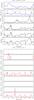 |
Fig. 6 Same as Fig. 3 but in the case of a larger orbital separation between the NS and the supergiant companion. In this case the separation corresponds to 25.6 days assuming a NS of 1.4 M⊙ and a supergiant of 34 M⊙. |
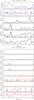 |
Fig. 7 Same as Fig. 6 but for a NS spin period of 1000 s. The magnetic field strength was not changed. |
In this section we present similar results to those in Sect. 4.1, but in the case of a larger orbital separation between the NS and the supergiant companion. In Figs. 6−8, we show the results of the previous calculations reported in Figs. 3–5 extended to the longer orbital period case. As can be seen by comparing each pair of figures, the qualitative discussion presented for the different magnetic field and spin period cases from Sect. 4.1 still holds and the system in the different configurations experience similar accretion regimes.
The main difference from the shorter orbital period case is that at larger distances from the supergiant companion, the variations in the density and velocity of the clumpy wind are much shallower. This leads to a substantially less pronounced variability, with X-ray outbursts becoming less and less frequent and low level activity intervals more and more prolonged in time. It is particularly interesting to note that the X-ray variability observed in the case with the higher magnetic field and longer spin period (μ33 = 0.1 and Ps3 = 1, see Fig. 8) is still the one that most closely resembles the behavior typical of SFXTs, with fewer and fewer prominent outbursts arising during periods of longer and longer low level X-ray emission.
5. Discussion and conclusions
In this paper we presented a first attempt to take into account the effects of the magnetic and centrifugal gating mechanisms during the accretion of a highly structured stellar wind onto a NS hosted in a SGXB. We showed that the magnetic field properties and the spin period of the compact object dramatically affect the X-ray luminosity released by the system.
The nonstationary wind model we adopted in this work is well known to provide reasonably good predictions for the X-rays observed from massive stars. Although the density and velocity variations derived from this model might need to be revised in the future when 2D/3D models are available (see Sect. 1), the coupling of these variations with all the gating accretion regimes proposed originally by B08 allowed us to investigate how the transitions between these regimes can be triggered in the clumpy environment of a wind-fed SGXB. We have also been able to study which X-ray luminosity and variability pattern can be expected as a function of the NS spin period, magnetic field, and orbital period. Based on all the cases analyzed in Sect. 4, we first highlighted the fact that the introduction of the gating mechanisms led to a substantial reduction of the average system X-ray emission compared to that computed from a simplified Bondi-Hoyle accretion scenario, even in those cases in which modest magnetic field values (~1012 G) and short spin periods (~10 s) are assumed for the compact object. This suggests that calculations of the X-ray luminosity released by NS wind-fed binaries in which the effect of the gating mechanisms is not taken into account could be significantly overestimated.
We also found that the combination of a longer spin period and a higher magnetic field might more easily lead to an SFXT-like behavior, i.e., with sporadic bright outbursts emerging during periods of a much fainter X-ray emission (as previously discussed by B08). It is also worth noting that the reduction of the mass accretion rate onto the compact object strongly increases with the intensity of the magnetic field, thus strengthening the idea that highly magnetized NSs can be hosted in SFXTs as the inhibition of accretion has been convincingly identified as a key ingredient to explain the subluminosity of all sources in this class compared to classical SGXBs (Lutovinov et al. 2013; Bozzo et al. 2015). We also note that the similarity observed in the transitions between different accretion regimes for systems with smaller or larger orbital periods in Sects. 4.1 and 4.2 is in agreement with the observational evidence that SFXTs with orbital separations spanning from a few to several days display remarkably similar behaviors in the X-ray domain (Romano et al. 2014a; Sidoli et al. 2016).
In general, it is difficult to reproduce the behavior of classical SGXBs within the assumption of a NS accreting from the extremely clumpy wind in Sect. 2. The large density and velocity variations produced by the adopted clumpy wind model lead in all cases to a more pronounced variability than that observed from these systems. However, it was highlighted in Sect. 4 how placing the NS at a larger distance from the supergiant companion improves the similarity between simulations and the observed behaviors of both classical SGXBs and SFXTs, as in these cases the stellar wind is characterized by smoother density and velocity contrasts. With future multidimensional stellar wind models featuring less extreme clump properties, it is thus likely that the gating accretion scenario can be used to explain the difference between classical SGXBs and SFXTs by fine-tuning only the NS parameters.
It must be noted here that, in addition to the limitations of the 1D clumpy wind model, the present simulations are also affected by a number of other simplifications. In particular, the NS is placed in all cases at a certain distance from the supergiant and neither its gravitational field nor the X-rays released as a consequence of the accretion produce any feedback onto the stellar wind. We know from hydrodynamics simulations of wind-fed systems that the gravitational field of the compact object can largely distort the accretion flow and produce significant density and velocity variations close to the compact object. These variations can thus enhance the X-ray variability already produced by the presence of the clumps and the effect of the gating mechanisms (Blondin et al. 1991; Blondin 1994; Manousakis & Walter 2015). The photoionization of the stellar wind by the X-rays emitted from the accreting NS can also produce significant variations in the physical properties of the wind, including its composition and velocity, the most recent investigations of which have been presented by Krtička et al. (2012) and Krtička et al. (2015). These authors have shown that the supergiant wind velocity can drop significantly close to the compact object or also be completely halted by the X-ray irradiation if the photoionization inhibits the radiative acceleration down to the surface of the supergiant star. As the accretion radius and the magnetospheric radius are highly sensible to variations in the wind velocity (see Eqs. (1), (2), (10), and (12)), we expect that the switches between different accretion regimes can also be affected by the photoionization. However, calculating the reciprocal feedback between photoionization effects and gating accretion mechanisms in the case of a strongly inhomogeneous stellar wind would require the development of an extremely challenging full 3D magneto-hydrodynamical treatment of the problem. This has not been possible so far. As the X-ray irradiation of the stellar wind depends on the orbital separation of the system, it is clear that our simplified treatment of the problem would become less and less accurate for shorter orbital period systems or for binaries with large eccentricities. For this reason we did not consider the case of orbital periods shorter than ~9 days. We also note that short orbital period systems (≲3−5 days) at X-ray luminosities of ≲1036−37 erg s-1 could develop temporary accretion disks (Ducci et al. 2010; Romano et al. 2015), whose effect on the accretion process cannot be taken into account in the present version of our computations. We plan to include all these complications in future improved versions of the simulations presented here.
Other mechanisms have been proposed to inhibit the accretion in the SFXTs and to produce sporadic bright outbursts (see Shakura et al. 2014).
We approximated a−RM ≃ a, which is satisfied for a very wide range of parameters of interest for the HMXBs considered in this paper.
In this paper we will only consider accretion processes over shorter timescales (hours to days) than those on which we expect the NS spin period to change significantly as a consequence of accretion torques (see B08).
Acknowledgments
This publication was motivated by a team meeting sponsored by the International Space Science Institute at Bern, Switzerland. E.B. and L.O. thank ISSI for the financial support during their stay in Bern. We thank an anonymous referee for the useful comments.
References
- Blondin, J. M. 1994, ApJ, 435, 756 [NASA ADS] [CrossRef] [EDP Sciences] [Google Scholar]
- Blondin, J. M., Stevens, I. R., & Kallman, T. R. 1991, ApJ, 371, 684 [NASA ADS] [CrossRef] [Google Scholar]
- Bodaghee, A., Tomsick, J. A., Rodriguez, J., et al. 2010, ApJ, 719, 451 [NASA ADS] [CrossRef] [Google Scholar]
- Bozzo, E., Falanga, M., & Stella, L. 2008, ApJ, 683, 1031 [NASA ADS] [CrossRef] [Google Scholar]
- Bozzo, E., Stella, L., Ferrigno, C., et al. 2010, A&A, 519, A6 [NASA ADS] [CrossRef] [EDP Sciences] [Google Scholar]
- Bozzo, E., Giunta, A., Cusumano, G., et al. 2011, A&A, 531, A130 [NASA ADS] [CrossRef] [EDP Sciences] [Google Scholar]
- Bozzo, E., Romano, P., Ducci, L., Bernardini, F., & Falanga, M. 2015, Adv. Space Res., 55, 1255 [NASA ADS] [CrossRef] [Google Scholar]
- Davidson, K., & Ostriker, J. P. 1973, ApJ, 179, 585 [NASA ADS] [CrossRef] [Google Scholar]
- Dessart, L., & Owocki, S. P. 2003, A&A, 406, L1 [NASA ADS] [CrossRef] [EDP Sciences] [Google Scholar]
- Dessart, L., & Owocki, S. P. 2005, A&A, 437, 657 [NASA ADS] [CrossRef] [EDP Sciences] [Google Scholar]
- Ducci, L., Sidoli, L., & Paizis, A. 2010, MNRAS, 408, 1540 [NASA ADS] [CrossRef] [Google Scholar]
- Feldmeier, A. 1995, A&A, 299, 523 [NASA ADS] [Google Scholar]
- Feldmeier, A., Kudritzki, R.-P., Palsa, R., Pauldrach, A. W. A., & Puls, J. 1997a, A&A, 320, 899 [NASA ADS] [Google Scholar]
- Feldmeier, A., Puls, J., & Pauldrach, A. W. A. 1997b, A&A, 322, 878 [NASA ADS] [Google Scholar]
- Grebenev, S. A., & Sunyaev, R. A. 2007, Astron. Lett., 33, 149 [NASA ADS] [CrossRef] [Google Scholar]
- Illarionov, A. F., & Sunyaev, R. A. 1975, A&A, 39, 185 [NASA ADS] [Google Scholar]
- in’t Zand, J. J. M. 2005, A&A, 441, L1 [NASA ADS] [CrossRef] [EDP Sciences] [Google Scholar]
- Krtička, J., Kubát, J., & Skalický, J. 2012, ApJ, 757, 162 [NASA ADS] [CrossRef] [Google Scholar]
- Krtička, J., Kubát, J., & Krtičková, I. 2015, A&A, 579, A111 [NASA ADS] [CrossRef] [EDP Sciences] [Google Scholar]
- Lipunov, V. M. 1987, Ap&SS, 132, 1 [NASA ADS] [CrossRef] [Google Scholar]
- Lipunov, V. M., Börner, G., & Wadhwa, R. S. 1992, Astrophysics of Neutron Stars (Springer-Verlag) [Google Scholar]
- Lucy, L. B., & White, R. L. 1980, ApJ, 241, 300 [NASA ADS] [CrossRef] [Google Scholar]
- Lutovinov, A. A., Revnivtsev, M. G., Tsygankov, S. S., & Krivonos, R. A. 2013, MNRAS, 431, 327 [NASA ADS] [CrossRef] [Google Scholar]
- Manousakis, A., & Walter, R. 2015, A&A, 575, A58 [NASA ADS] [CrossRef] [EDP Sciences] [Google Scholar]
- Negueruela, I., Smith, D. M., Reig, P., Chaty, S., & Torrejón, J. M. 2006, in The X-ray Universe 2005, ed. A. Wilson, ESA SP, 604, 165 [NASA ADS] [Google Scholar]
- Negueruela, I., Smith, D. M., Torrejon, J. M., & Reig, P. 2007, ESA SP-622, 255 [Google Scholar]
- Oskinova, L. M., Feldmeier, A., & Hamann, W.-R. 2006, MNRAS, 372, 313 [NASA ADS] [CrossRef] [Google Scholar]
- Oskinova, L., Hamann, W.-R., Todt, H., & Sander, A. 2012a, in Proc. Scientific Meeting in Honor of Anthony F. J. Moffat, eds. L. Drissen, C. Rubert, N. St-Louis, & A. F. J. Moffat, ASP Conf. Ser., 465, 172 [Google Scholar]
- Oskinova, L. M., Feldmeier, A., & Kretschmar, P. 2012b, MNRAS, 421, 2820 [NASA ADS] [CrossRef] [Google Scholar]
- Paizis, A., & Sidoli, L. 2014, MNRAS, 439, 3439 [NASA ADS] [CrossRef] [Google Scholar]
- Puls, J., Vink, J. S., & Najarro, F. 2008, A&ARv, 16, 209 [NASA ADS] [CrossRef] [EDP Sciences] [Google Scholar]
- Romano, P. 2015, J. High Energy Astrophysics, 7, 126 [Google Scholar]
- Romano, P., Sidoli, L., Mangano, V., et al. 2008, ApJ, 680, L137 [NASA ADS] [CrossRef] [Google Scholar]
- Romano, P., La Parola, V., Vercellone, S., et al. 2011, MNRAS, 410, 1825 [NASA ADS] [Google Scholar]
- Romano, P., Mangano, V., Ducci, L., et al. 2013, Adv. Space Res., 52, 1593 [NASA ADS] [CrossRef] [Google Scholar]
- Romano, P., Ducci, L., Mangano, V., et al. 2014a, A&A, 568, A55 [NASA ADS] [CrossRef] [EDP Sciences] [Google Scholar]
- Romano, P., Krimm, H. A., Palmer, D. M., et al. 2014b, A&A, 562, A2 [NASA ADS] [CrossRef] [EDP Sciences] [Google Scholar]
- Romano, P., Bozzo, E., Mangano, V., et al. 2015, A&A, 576, L4 [NASA ADS] [CrossRef] [EDP Sciences] [Google Scholar]
- Shakura, N., Postnov, K., Sidoli, L., & Paizis, A. 2014, MNRAS, 442, 2325 [NASA ADS] [CrossRef] [Google Scholar]
- Sidoli, L., Romano, P., Mangano, V., et al. 2008, ApJ, 687, 1230 [NASA ADS] [CrossRef] [Google Scholar]
- Sidoli, L., Romano, P., Esposito, P., et al. 2009, MNRAS, 400, 258 [NASA ADS] [CrossRef] [Google Scholar]
- Sidoli, L., Esposito, P., & Ducci, L. 2010, MNRAS, 409, 611 [NASA ADS] [CrossRef] [Google Scholar]
- Sidoli, L., Paizis, A., & Postnov, K. 2016, MNRAS, 457, 3693 [NASA ADS] [CrossRef] [Google Scholar]
- Šurlan, B., Hamann, W.-R., Aret, A., et al. 2013, A&A, 559, A130 [NASA ADS] [CrossRef] [EDP Sciences] [Google Scholar]
- Walter, R., & Zurita Heras, J. 2007, A&A, 476, 335 [Google Scholar]
- Walter, R., Lutovinov, A. A., Bozzo, E., & Tsygankov, S. S. 2015, A&ARv, 23, 2 [NASA ADS] [CrossRef] [Google Scholar]
Appendix A: Bondi-Hoyle accretion
In the Bondi-Hoyle accretion scenario adopted previously by Oskinova et al. (2012b), the authors followed the simplified treatment proposed by Davidson & Ostriker (1973) in which a NS is traveling with a relative speed vrel through a gas with density ρ. The mass accretion rate is given in this case by  (A.1)where the quantities Ra, vrel, and ρw are the same as those introduced in Sect. 3. The factor ζ ~ 1 is included to take into account numerical corrections due to the radiation pressure and the finite cooling time of the gas. Combining Eq. (A.1) and (1), the following can be obtained:
  (A.2)In these equations, ρw is assumed to be the time dependent density of the wind provided by the clumpy wind code described in Sect. 2. Oskinova et al. (2012b) did not neglect the NS orbital velocity compared to the wind velocity, and thus
  (A.3)where the orbital velocity of the NS, vX, is given by
  (A.4)The X-ray luminosity of an accreting neutron star in this simplified scenario can thus be expressed as
  (A.5)where c is the speed of light and η ~ 0.1 is a numerical constant introduced to take into account unknown geometrical aspects of the accretion process. The value computed through Eq. (A.5) is reported in all the bottom panels of Figs. 3−8 with a solid magenta line.
All Figures
|
Fig. 1 Snapshot at a fixed time of the density stratification (upper panel) and velocity field (lower panel) of the stellar wind in a O9.5 supergiant star, as predicted by time-dependent hydrodynamic simulations described in Sect. 2. The upper panel shows that the wind density can change by several orders of magnitude owing to the presence of clumps. The corresponding strong wind velocity jumps are visible in the lower panel. |
| In the text | |
|
Fig. 2 Schematic flow of the conditions that are considered within the clumpy wind code to establish which is the relevant accretion regime for the system at each time step and how the total X-ray luminosity should be calculated. |
| In the text | |
|
Fig. 3 Results of the simulations of the accretion onto a NS using the nonstationary wind model introduced in Sect. 2 and taking into account the gating accretion mechanisms described in Sect. 3. The system parameters adopted in the simulation are shown above each figure (a separation of 2.5 R∗ corresponds to an orbital period of 9.1 days). Left figure: wind velocity and density as a function of time, and all relevant radii to be determined in the gating accretion model. In the density panel we also show the value of the critical density in Eq. (13) (red dashed line). Right figure (all panels): different contributions to the total X-ray luminosity of the system, which is given in the bottom panel, together with the corresponding X-ray luminosity that would be achieved by assuming the simplest Bondi-Hoyle scenario (magenta solid line; see Appendix A). Empty regions in each panel represent time intervals in which the corresponding quantity is not calculated because the source is not in that specific accretion regime (or is out of scale and thus negligible for the overall luminosity budget; see Sect. 4 for details). |
| In the text | |
|
Fig. 4 Same as Fig. 3 but for a NS spin period of 1000 s. The magnetic field strength was not changed. |
| In the text | |
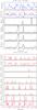 |
Fig. 5 Same as Fig. 3 but for a NS spin period of 1000 s and a magnetic field strength of 1014 G. |
| In the text | |
|
Fig. 6 Same as Fig. 3 but in the case of a larger orbital separation between the NS and the supergiant companion. In this case the separation corresponds to 25.6 days assuming a NS of 1.4 M⊙ and a supergiant of 34 M⊙. |
| In the text | |
|
Fig. 7 Same as Fig. 6 but for a NS spin period of 1000 s. The magnetic field strength was not changed. |
| In the text | |
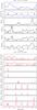 |
Fig. 8 Same as Fig. 6 but for a NS spin period of 1000 s and a magnetic field strength of 1014 G. |
| In the text | |
Current usage metrics show cumulative count of Article Views (full-text article views including HTML views, PDF and ePub downloads, according to the available data) and Abstracts Views on Vision4Press platform.
Data correspond to usage on the plateform after 2015. The current usage metrics is available 48-96 hours after online publication and is updated daily on week days.
Initial download of the metrics may take a while.