| Issue |
A&A
Volume 589, May 2016
|
|
|---|---|---|
| Article Number | A83 | |
| Number of page(s) | 10 | |
| Section | Numerical methods and codes | |
| DOI | https://doi.org/10.1051/0004-6361/201528052 | |
| Published online | 18 April 2016 | |
A new method for the inversion of atmospheric parameters of A/Am stars⋆,⋆⋆
1 Department of Physics and Astronomy, Notre Dame University-Louaize, PO Box 72, Zouk Mikaël, Lebanon
e-mail: This email address is being protected from spambots. You need JavaScript enabled to view it.
2 Université de Toulouse, UPS-Observatoire Midi-Pyrénées, IRAP, 31000 Toulouse, France
3 CNRS, Institut de Recherche en Astrophysique et Planétologie, 14 av. E. Belin, 31400 Toulouse, France
4 LESIA, UMR 8109, Observatoire de Paris, place J. Janssen, Meudon, France
5 Laboratoire Lagange, Université de Nice Sophia, Parc Valrose, 06100 Nice, France
Received: 28 December 2015
Accepted: 2 March 2016
Abstract
Context. We present an automated procedure that simultaneously derives the effective temperature Teff, surface gravity log g, metallicity [Fe/H], and equatorial projected rotational velocity vsini for “normal” A and Am stars. The procedure is based on the principal component analysis (PCA) inversion method, which we published in a recent paper .
Aims. A sample of 322 high-resolution spectra of F0-B9 stars, retrieved from the Polarbase, SOPHIE, and ELODIE databases, were used to test this technique with real data. We selected the spectral region from 4400−5000 Å as it contains many metallic lines and the Balmer Hβ line.
Methods. Using three data sets at resolving powers of R = 42 000, 65 000 and 76 000, about ~6.6 × 10⁶ synthetic spectra were calculated to build a large learning database. The online power iteration algorithm was applied to these learning data sets to estimate the principal components (PC). The projection of spectra onto the few PCs offered an efficient comparison metric in a low-dimensional space. The spectra of the well-known A0- and A1-type stars, Vega and Sirius A, were used as control spectra in the three databases. Spectra of other well-known A-type stars were also employed to characterize the accuracy of the inversion technique.
Results. We inverted all of the observational spectra and derived the atmospheric parameters. After removal of a few outliers, the PCA-inversion method appeared to be very efficient in determining Teff, [Fe/H], and vsini for A/Am stars. The derived parameters agree very well with previous determinations. Using a statistical approach, deviations of around 150 K, 0.35 dex, 0.15 dex, and 2 km s-1 were found for Teff, log g, [Fe/H], and vsini with respect to literature values for A-type stars.
Conclusions. The PCA inversion proves to be a very fast, practical, and reliable tool for estimating stellar parameters of FGK and A stars and for deriving effective temperatures of M stars.
Key words: stars: fundamental parameters / stars: early-type / methods: numerical
Based on data retrieved from the Polarbase, SOPHIE, and ELODIE archives.
Table 2 is only available at the CDS via anonymous ftp to cdsarc.u-strasbg.fr (130.79.128.5) or via http://cdsarc.u-strasbg.fr/viz-bin/qcat?J/A+A/589/A83
© ESO, 2016
1. Introduction
Sky and ground-based surveys can produce hundreds of terabytes (TB) and up to 100 (or more) petabytes (PB), both in the image data archive and in the object catalogues (Borne 2013). For instance, the ESA space mission Gaia (Perryman et al. 2001), launched in December 2013, is expected to produce a final archive of about 1 PB (1015 bytes) through five years of exploration. The Large Synoptic Survey Telescope (LSST) project will conduct a ten-year survey of the sky that will deliver about 15 terabytes (TB) of raw data per night (Kantor et al. 2007). The total amount of data collected over the ten years of operation will be 60 PB, and processing these data will produce a 15 PB catalogue database. The need for methods that can handle and analyse this large amount of information is evident.
Principal component analysis (PCA) has been used to invert stellar spectra to determine stellar fundamental parameters of stars (Bailer-Jones et al. 1998; Re Fiorentin et al. 2007; Paletou et al. 2015b,c). This technique has proven to be a fast and reliable tool to invert observed high-resolution spectra. Unlike classical techniques such as least-squares fitting, PCA is based on a dimensionality reduction for the fast search of the nearest neighbour of an observed spectrum in a learning database. This technique can become obviously advantageous when dealing with large number of extended spectra collected at various spectral resolutions during sky surveys such as the Sloan Digital Sky Survey (SDSS; York et al. 2000), the RAdial Velocity Experiment (RAVE; Steinmetz 2003; Munari et al. 2005), and more recently the Gaia ESO Survey (GES; Gilmore et al. 2012).
A description of the PCA-based inversion technique for stellar parameters that we use can be found in Paletou et al. (2015b), where the authors applied this technique to derive fundamental parameters from high-resolution spectra of FGK stars. Paletou et al. (2015c) have shown that the range of application of the principal component analysis-based inversion method can be extended to dwarf M stars to derive effective temperatures.
We extend the work of Paletou et al. (2015b) to A-type stars whose effective temperatures range between 7000 and 10 000 K. A large variety of physical processes are at play in the envelopes of A/Am stars. Chemical peculiarity and pulsation are observed among main-sequence A and F stars. Chemical peculiarity is a signature of the occurrence of transport processes competing with radiative diffusion (Zahn 2005; Richer et al. 2000; Richard et al. 2001, 2002; Vick et al. 2010). Chemical peculiarity exist in different ways in A-type stars (Am, Ap, λ Bootis stars...). These peculiarities set constraints on self-consistent evolutionary models of these objects, including various particle transport processes (Gebran et al. 2008; Gebran & Monier 2008; Gebran et al. 2010). The stellar atmospheric parameters are the prerequisites to any detailed abundance analysis, and for that reason, these parameters should be derived with good accuracy.
To do so, we calculated around 6.6 × 10⁶ synthetic spectra and used them as three learning databases. These synthetic spectra were compared to a collection of observed spectra to find the best global fit between the two sets. The A-type stars spectra that we analysed were selected from the PolarBase1 (Petit et al. 2014) stellar library at two different resolutions (R ~ 65 000 and R ~ 76 000), and from the SOPHIE2 and ELODIE3 archives (Moultaka et al. 2004) (R ~ 75 000 and 42 000, respectively). We restricted our study to the wavelength range 4400−5000 Å. In this region, free from telluric lines, we can find many metallic lines and mostly many iron transitions (Fe i and Fe ii) with accurate atomic data. The Balmer line Hβ around ~4860 Å is also present in this spectral range. As mentioned by Smalley (2005), the advantage of the global spectral fitting technique is that it can be automated for a very large number of stellar observations. It can also be used for low-resolution spectra or spectra of fast rotators, where line blending is important (vsini can go up to 300 km s-1 for A-type stars). Dealing with large multi-dimensional grid of synthetic spectra, the combination of the metallic and Balmer lines is essential for the derivation of the effective temperature Teff, surface gravity log g, metallicity [Fe/H], and projected equatorial rotational velocity vsini (Smalley 2005).
As a result of their sensitivity to effective temperature and surface gravity, hydrogen line profiles should be included in all automatic procedures based on spectral fitting to obtain realistic atmospheric parameters for stars hotter than 5500 K (Ryabchikova et al. 2015). The Balmer lines in B to F stars are in general well matched by LTE computations, and they are practically identical to the non-LTE predictions (Przybilla & Butler 2004). The region around Hβ was chosen because it harbours several iron lines with accurate atomic parameters. The Balmer lines provide an excellent diagnostic of Teff for stars cooler than ~8000 K (Gray 1992; Heiter et al. 2002). For stars hotter than 8000 K, Balmer line profiles, in particular their wings, are sensitive to both temperature and gravity (Gray 1992; Smalley 2005). Metal line diagnostics are also good indicators of Teff, log g, and [Fe/H] as the best-fit synthetic spectrum corresponds to the spectrum that yields the same abundance for different ionization stages of the same element (ionization balance) and in the same abundance for all excitation potentials of the same element in a given ionization stage (excitation potential). On the other hand, lines such as the Mg ii triplet around 4481 Å and the Fe ii lines between 4500 and 4530 Å are excellent indicators of vsini (see for example Royer et al. 2014). For all the above mentioned reasons, we applied the global spectral fitting technique to the whole spectral range from 4400 and 5000 Å. The derived parameters are obviously model dependent, but the models that we are using (Sect. 2.2) are well suited to describe the atmospheres and spectra of “normal” A and Am stars.
The selection of the observed spectra and construction of the learning databases are detailed in Sect. 2. The PCA and the derivation of the eigenvectors and coefficients are recalled in Sect. 3. Radial velocity correction and re-normalization of the spectra are discussed in Sect. 4. The results of the inversion are presented in Sect. 5. A few outliers have been analysed in detail in Sect. 6. Discussion and conclusion are gathered in Sect. 7.
2. Observations and learning database
2.1. Target selection
The PolarBase contains reduced stellar spectra collected with the NARVAL and ESPaDOnS high-resolution spectropolarimeters. These two spectropolarimeters are mounted on the 2 m aperture Télescope Bernard Lyot (TBL) in France and on the 3.6 m aperture CFHT telescope in Hawaii, respectively. Both instruments have a spectral resolving power of 65 000 in polarimetric mode and 76 000 when used for classical spectroscopy. As a first step, we have selected all high-resolution Echelle spectra of stars whose spectral type ranges from F0 up to B9 from the database at two different resolutions and in spectroscopy mode only. Fifty spectra were thus retrieved.
We have also retrieved A-type stars spectra from the ELODIE and SOPHIE archives. These archives are on-line databases of high-resolution Echelle spectra and radial velocities. The ELODIE is a fiber-fed, cross-dispersed Echelle spectrograph that was attached to the 1.93-m telescope at Observatoire de Haute-Provence (OHP; Baranne et al. 1996). The ELODIE recorded in a single exposure a spectrum extending from 3850 Å to 6811 Å at a resolving power of about 42 000 on a relatively small CCD (1024 × 1024). SOPHIE is the Echelle spectrograph mounted on the 1.93-m telescope at the OHP since September 2006. SOPHIE spectra stretch from 3870 to 6940 Å in 39 orders with two different spectral resolutions: the high-resolution mode (HR; R ~ 75 000) and the high efficiency mode (HE; R = 39 000). All the observations that we used were observed in the HR mode at the same resolution of NARVAL spectra. Spectra of 279 stars, with signal-to-noise ratio larger than 100, were downloaded from the SOPHIE and ELODIE archives. Overall, we selected 322 stars for our study. The identifications of the selected stars are collected in Table 2. These data correspond to PolarBase, ELODIE, and SOPHIE spectra, respectively. Inverted effective temperatures, surface gravities, projected equatorial rotational velocities, metallicities, and radial velocities are collected in this table (see Sect. 5).
2.2. Learning database
The learning database was constructed using synthetic spectra following Paletou et al. (2015c). Three sets of grids were used, at a resolution of 65 000, 76 000, and 42 000, corresponding to the resolution of Polarbase, ELODIE and SOPHIE spectra, respectively. These three grids are identical in terms of the parameters (Teff, log g, [Fe/H], vsini, ξt), and only the resolution differs. Line-blanketed ATLAS9 model atmospheres (Kurucz 1992) were calculated for the purpose of this work. ATLAS9 models are LTE plane parallel and assume radiative and hydrostatic equilibrium. This ATLAS9 version uses the opacity distribution function (ODF) of Castelli & Kurucz (2003). We included convection in the atmospheres of stars cooler than 8500 K. Convection was treated using a mixing length parameter of 0.5 for 7000 K≤Teff ≤ 8500 K, and 1.25 for Teff≤ 7000 K, following Smalley’s (2004) prescriptions.
The grid of synthetic spectra was computed using SYNSPEC48 (Hubeny & Lanz 1992). The effective temperatures of the model atmospheres range from 6800 and 11 000 K with a step of 100 K, and logarithm of surface gravities between 2.0 and 5.0 with a step of 0.1 dex, respectively. The projected equatorial rotational velocities vsini were varied from 0 up to 300 km s-1 with a non-constant step (2, 5, and 10 km s-1), and the metallicity was scaled from −2.0 dex up to +2.0 dex with respect to the Grevesse & Sauval (1998) solar value with a step of 0.1 dex. The synthetic spectra were computed from 4400 Å up to 5000 Å with a wavelength step of 0.05 Å. This range contains many moderate and weak metallic lines in different ionization stages. These weak metallic lines (indicators for vsini and [Fe/H]) and the Balmer line (indicator for Teff and log g) are not sensitive to small changes of the microturbulent velocity. For that reason, we fixed the microturbulent velocity (ξt) to 2.0 km s-1 in all models. This value corresponds to the average microturbulent velocity in A-type stars (Gebran et al. 2014). The line list used in the synthetic spectra calculation was constructed from Kurucz gfhyperall.dat4 and modified with more recent and accurate atomic data retrieved from the VALD5 and the NIST6 databases. At each resolution, we ended up with ~2.2 million spectra as a learning database.
3. Principal component analysis
Our usage of the PCA for the inversion process is influenced by the work of Rees et al. (2000) and Paletou et al. (2015b,c). As mentioned in Sect. 1, the PCA is a reduction of dimensionality technique that retains the variation present in the data set (Jolliffe 1986) as much as possible. It searches for basis vectors that represent most of the variance in a given database. The reduction of dimensionality allowed by the PCA is directly used to build a specific metric from which a nearest-neighbour(s) search is made between an observed data set (observed spectra in the present work) and the content of a learning database (synthetic spectra in the present work). The learning database could be constructed with a set of observed spectra with well-known parameters (Paletou et al. 2015b). The PCA becomes mainly advantageous when dealing with high- and low-resolution spectra that cover a very broad bandwidth as the reduction of dimensionality allows a very fast processing of the data. In what follows, we describe the characteristics of this technique in the context of our study.
3.1. Nearest neighbour search
Representing the learning database in a matrix S of size Nspectra = 2.2 × 10⁶ by Nλ = 12 000,  is the average of S along the Nspectra-axis. Then, we derive the eigenvectors ek(λ) of the variance-covariance matrix C defined as
  (1)with a dimension of Nλ × Nλ. These eigenvectors of the symmetric C matrix are then sorted in decreasing eigenvalues magnitude; they are more usually referred to as “principal components”. Each spectrum of the data set S is represented by a small number of coefficients pjk defined as
  (2)The main point of reducing the dimensionality is the selection of kmax ≪ Nλ. We show in Sect. 3.2 that kmax = 12 is a reasonable choice.
To follow the same notation as in Paletou et al. (2015b), we denote the observed spectrum by O(λ) having the same wavelength range and sampling as the learning data set spectra. At this stage, the observations should be corrected for radial velocity (details in Sect. 4). We compute the set of projection coefficients ϱk defined as  (3)The nearest neighbour is then found by minimizing a χ2 in the low-dimensional space of the coefficients
  (4)where j covers the number of synthetic spectra. The parameters of the synthetic spectrum with the minimum d are considered for the inversion.
3.2. Power iteration method
The derivation of the leading eigenvectors of C is the most critical step when performing PCA, and it becomes increasingly time consuming as the size of learning data set increases. Furthermore, techniques, such as singular value decomposition (SVD) that were used in previous studies, become inapplicable in this case as a result of computer memory shortage. In our particular case, at each of the three resolutions, the files containing the matrix S are ≈240 GB in size. To bypass this problem, we used an algorithm that is applicable independent of the size of the data set. We implemented the online power iteration algorithm (also called Von Mises iteration; Demmel 1997) to estimate the kmax principal components of the data set S. This algorithm reads and operates on synthetic spectra of the learning data set one by one, avoiding loading all the data at once. The procedure, moreover, does not need any typical matrix factorization such as SVD, and is efficient when applied to large data sets (Roweis 1998). The procedure consists of the following.
First we find the eigenvector e1 with a maximal eigenvalue λ1 (i.e. the first principal component), by iterating 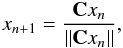 (5)with an initial random non-zero vector x0. Practically Cxn cannot be computed using standard technique as one should load the full data set S at once to calculate C. To overcome this problem, we evaluate “Cxn” for each iteration on xn while operating on each spectrum at a time by performing
 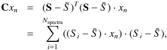 (6)where Si is the ith spectrum in the data set S. The xn iterations converge to the eigenvector e1 that corresponds to the largest eigenvalue.
Once we find a good approximation for e1, we perform the Gram-Schmidt process to remove the contribution of e1 from S by computing ![Mathematical equation: \begin{equation} \textbf{S}_1= \textbf{S}-[(\textbf{S}-\bar{S})\cdot e_1]e_1. \end{equation}](/articles/aa/full_html/2016/05/aa28052-15/aa28052-15-eq54.png) (7)Again, the above should be performed iteratively over each spectrum. Next, to compute e2, the power method (Eq. (5)) is performed on
(7)Again, the above should be performed iteratively over each spectrum. Next, to compute e2, the power method (Eq. (5)) is performed on 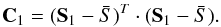 (8)Once e2 is estimated, the Gram-Schmidt process is applied again to yield
 ![Mathematical equation: \begin{equation} \textbf{S}_2=\textbf{S}_1 - [(\textbf{S}_1-\bar{S})\cdot e_2] e_2 . \end{equation}](/articles/aa/full_html/2016/05/aa28052-15/aa28052-15-eq57.png) (9)And so on, until we compute all the needed eigenvectors. To determine the optimal number of iterations needed for the derivation of the eigenvectors, we constructed several smaller databases and derived their respective eigenvectors using the SVD technique and the power iteration. For each database, the derived eigenvectors from both techniques were compared. Using power iteration, 25 iterations were required to reach a relative difference between eigenvectors smaller than 0.1%. The use of power iteration allowed the increase of the number of spectra in the learning database by a factor of 10 (200 000 in case of the SVD to 2 200 000 in case of power iteration).
(9)And so on, until we compute all the needed eigenvectors. To determine the optimal number of iterations needed for the derivation of the eigenvectors, we constructed several smaller databases and derived their respective eigenvectors using the SVD technique and the power iteration. For each database, the derived eigenvectors from both techniques were compared. Using power iteration, 25 iterations were required to reach a relative difference between eigenvectors smaller than 0.1%. The use of power iteration allowed the increase of the number of spectra in the learning database by a factor of 10 (200 000 in case of the SVD to 2 200 000 in case of power iteration).
Only the first 12 eigenvectors were considered and that was justified by the calculation of the reconstruction error of the spectra defined as 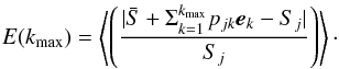 (10)Using only 12 eigenvectors, the average reconstruction error is found to be smaller than 1%, a result similar to that derived in Paletou et al. (2015b).
4. Preparation of the observed spectra
In order to adjust a synthetic spectrum to an observed spectrum, lines of both spectra should be aligned, as accurately as possible, on the same wavelength scale and both fluxes should be at the same level. The flux matching is achieved by rectifying the observed and synthetic spectra to their local continua.
4.1. Radial velocity correction
A wavelength shift between observations and synthetic spectra could drastically affect the derived parameters of the first neighbour. Paletou et al. (2015b) showed that the radial velocity vr should be known to an accuracy of c/ 4R, where c is the speed of light in vacuum. This requirement translates into a velocity accuracy of ~1 km s-1 needed at a spectral resolution of 76 000. We corrected all the spectra from radial velocity (given in the last column of Table 2) before the inversion procedure. The radial velocities were determined with the classical cross-correlation technique originally described by Tonry & Davis (1979). The observed spectra were cross correlated using a synthetic template, in the same wavelength range, corresponding to the parameters Teff = 8500 K, log g = 4.0 dex, [Fe/H] = 0, and vesini = 0 km s-1. Many of the Fe ii, Cr ii, Ti ii, and Mg ii atomic lines are mainly present in all sub-types of A-type stars (from A0 to A9). The wavelength of the Fe ii lines in the 4500−4550 Å region are accurately measured to within ~0.01 Å according to the NIST database. For that reason, the selected template corresponds to a typical A5V type star.
4.2. Renormalization of the flux
On the other hand, we also noticed that the flux normalization procedure is critical in this work and that an improper normalization could affect drastically the derived parameters. We proceeded using Gazzano et al. (2010)’s procedure to correct for this effect. Each originally normalized observed spectrum was divided by the synthetic spectrum calculated with the first inverted atmospheric parameters (Teff, log g, [Fe/H], and vsini). The residuals were then cleaned from lines with a sigma clipping, rejecting points above or below 1σ. The remaining points were fitted with a second degree polynomial. The observation was then divided by this polynomial in order to obtain a new normalized spectrum. This new spectrum was inverted again to find a new set of parameters. This procedure was repeated until the inverted parameters remained unchanged from one iteration to the next. The number of iterations depends on the original shape of the normalized observed spectrum. On average, ten iterations were sufficient to reach convergence. In Fig. 1, we show the application of the Gazzano et al. (2010) procedure to the inversion of the spectrum of HD 97230; only eight iterations were required in this example.
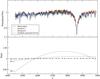 |
Fig. 1 Upper panel: continuum correction using eight iterations for the inversion of HD 97230. Only iterations 1 and 8 are shown for the sake of clarity, The initial observation is indicated with a solid line, the 1st iteration is indicated with dash-dotted line, the 8th iteration is indicated with double dash-dotted line, and the final best-fit synthetic spectrum is indicated with a dashed line. Lower panel: ratios between the re-normalized spectrum of the observation and the first neighbour best-fit synthetic spectrum for iterations 1, 2, and 8. |
5. A stars spectra inversions
5.1. Vega and Sirius A
The first tests were carried out using the two well-studied A-type stars, Vega (HD 172167, A0V) and Sirius A (HD 48915, A1m). The spectra of Vega were retrieved from the PolarBase and SOPHIE archive. The ESPaDOnS spectrum was inverted using the learning database at a resolution of 65 000, whereas the SOPHIE spectrum was inverted using the database at a resolution of 76 000. Both inversions yielded the same results for all parameters. We found for {Teff, log g, [Fe/H], vsini} values of {9500 K, 4.0 dex, −0.5 dex, 25 km s-1} , whereas the medians of the parameters found by querying Vizier7 are {9520 K, 3.98 dex, −0.53 dex, 23 km s-1}. The inverted parameters of Vega agree very well with all previous determinations, such as Takeda et al. (2008), Hill et al. (2010), and the fundamental effective temperature derived by Code et al. (1976) from the integrated flux and the angular diameter. Figure 2a shows the overall adjustment of four observed spectra of Vega with the first neighbour synthetic spectra. These spectra were observed at different epochs. The good agreement between the inverted metallicity and the projected equatorial rotational velocity of Vega with those from the catalogue can be seen in Fig. 2b, where we show the adjustment in the region sensitive to these two parameters. The spectrum of Sirius A was retrieved from the ELODIE database. This spectrum was inverted using the learning database at a resolution of 42 000. We found for {Teff, log g, [Fe/H], vsini} values of {9800 K, 4.2 dex, 0.2 dex, 18 km s-1} , whereas the medians of the parameters retrieved from a Vizier query are {9870 K, 4.30 dex, 0.36 dex, 15 km s-1}. This result is in very good agreement with previous findings such as Hill & Landstreet (1993), Takeda et al. (2009), and Landstreet (2011).
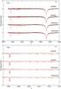 |
Fig. 2 First neighbour fit of synthetic spectra to the observed spectra for the four spectra of Vega, observed at different epochs, retrieved from PolarBase and SOPHIE databases. Observed spectra are shown in black and the synthetic spectra are shown in red. Part a) represents the overall spectrum, whereas part b) indicates the region sensitive to [Fe/H] and vsini. The wavelengths are in Å. Spectra were offset by arbitrary amounts. |
Table 2 shows the inverted parameters, the values that we retrieved from Vizier queries closest to our inverted values, and the median of queried catalogues values. All literature data were collected from Vizier catalogues using the ASTROQUERY8 Python modules (Paletou & Zolotukhin 2014). We kept the inverted parameters for all selected stars in this table even though many of these stars may be variables or binaries. Using Simbad queries, we listed, in the last column of Table 2, the peculiarity of the stars. Variables and binary systems were discarded in the characterization of the technique (Sect. 5.2).
The effective temperature is the only atmospheric parameter that can be retrieved from Vizier queries for all stars except for one exception. A small number of the selected stars do not have catalogues values for log g, vsini, and [Fe/H]. Figure 3 shows the inverted effective temperature for each spectrum retrieved from Polarbase as well as the range in the effective temperatures retrieved from the catalogues (box-plots) and the median. The number of values found in all catalogues retrieved in Vizier for each star also appears in this figure. We found that the inverted parameters agree well with those retrieved in the various catalogues. This agreement also applies to A-type stars spectra retrieved from ELODIE and SOPHIE archives (Table 2). However, we found several outliers that are discussed in detail in Sect. 6. These outliers are depicted with a symbol “*” in Table 2. Figure 4 shows an example of an overall spectral fitting between the first neighbour synthetic spectrum and the observation for several A-type stars of our study.
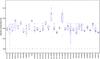 |
Fig. 3 Comparison between our estimate of effective temperatures (•), and the values we obtained from available Vizier catalogues, for PolarBase spectra. The latter collections are represented as classical boxplots. Objects we studied are listed along the horizontal axis. The number of values found among all Vizier catalogues are presented on a horizontal line around Teff ~ 4000 K. The horizontal bar inside each box indicates the median (Q2 value), while each box extends from first quartile, Q1, to third quartile Q3. Extreme values, still within a 1.5 times the interquartile range away from either Q1 or Q3, are connected to the box with dashed lines. Outliers are denoted by a “+” symbol. |
5.2. Evaluation of the results and comparison with literature data
In order to evaluate the efficiency of our method, first we removed from the analysis all peculiar stars, such as Ae/Be, Ap, variable (δ Scuti, γ Doradus variables...), and binary stars (eclipsing binaries, spectroscopic binaries...) as the models that we are using do not take such peculiarities into account. ATLAS12 (Kurucz 2005) model atmospheres, dealing with opacity sampling (OS), can better reproduce the distribution of the thermodynamical quantities in the atmosphere of chemically peculiar stars. Peculiarities of Am stars are not strong enough to alter the temperature distribution in their atmospheres (Gebran et al. 2008; Catanzaro & Balona 2012). For that reason, we are confident that ATLAS9 can be used for moderate chemical peculiarity.
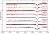 |
Fig. 4 First neighbour fit of synthetic spectra to the observed spectra. The wavelengths are in Å. Spectra were shifted up for clarity. |
We ended up with 182 classified “normal” A or Am stars. To assess an automated and objective comparison with already published values that one may find in Vizier@CDS, for instance, we found it reasonable to adopt specific weights for the set of values we could retrieve for each object. These weights directly rely on the spread of catalogued values. For some of the stars, dispersions in the catalogued values were noticed, and were severe up to thousands of Kelvin for Teff. As an example, HIP109119 has catalogued Teff ranging between 5309 K and 8970 K. On the other hand, some stars had only one or no catalogued values at all for a particular parameter. This would definitely add a bias to the error calculation. For that reason we used a statistical approach that gives less weight to stars with a large spread in the catalogued values. For a star i and a parameter ψ (ψ could be one of the following parameters: Teff, log g, [Fe/H], vsini), the difference between the inverted and median from the catalogued values of this parameter is weighted with the inverse of the interquartile range (IQR). IQR is defined as the difference between the third and first quartile of each set of values (IQR = Q3−Q1). The deviation for the parameter ψ is derived following:  (11)with wi derived for each star and each parameter as follows:
  (12)The associated standard deviation is found according to the following equation:
  (13)Stars with fewer than two catalogued values for a parameter ψ were omitted in the calculation of Δψw because of the zero value of their IQR. To estimate the parameters spread in the catalogued values for the remaining stars, we calculated the average IQR and the standard deviation. We found that, on average, the interquartile values for {Teff, log g, [Fe/H], vsini} are {550 K, 0.25 dex, 0.17 dex, 10.7 km s-1} with a standard deviations of {1200 K, 0.35 dex, 0.23 dex, 15.5 km s-1}. These numbers show that a large spread exists in the literature values, validating our approach in using a weighted mean. Applying Eq. (11), the derived deviations on the four parameters and their corresponding standard deviations are summarized in Cols. 2 and 3 of Table 1. Columns 4 to 11 of Table 1 show the absolute mean signed differences and standard deviations obtained by comparing our inverted parameters to the median and closest parameters in the catalogues from Vizier query for all stars (Cols. 4 to 7) and for the 19 reference stars (Cols. 8 to 11, see Sect. 5.2.1).
Average weighted deviations between our inverted parameters and catalogued values (Δw) with their respective standard deviation (σw).
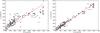 |
Fig. 5 Left panel: comparison between our inverted effective temperatures and the median of the catalogued effective temperatures. Right panel: comparison between our inverted effective temperatures and the closest of the catalogued effective temperatures. |
Effective temperature Teff
Figure 5 shows the comparison between our inverted effective temperature and the catalogued effective temperatures for the 182 classified “normal” A or Am stars. The left panel of Fig. 5 represents the comparison with the median of the catalogued values, whereas the right panel shows the comparison with the closest. There is a systematic trend noticed in the left plot of Fig. 5. This is partly because of the large spread in the catalogued data. By comparing our inverted Teff to the median value, we obtain an absolute mean signed difference of 110 K with a standard deviation of 630 K (Cols. 4 and 5 of Table 1). All stars (except HD 322676) have at least two values for catalogued Teff. These catalogued effective temperatures are based on different bibliographical references using distinct tools/techniques for their determination. Using spectroscopy, one should expect some differences between the derived effective temperatures and those determined with photometric techniques. The global spectral fitting that includes the Balmer lines provides an excellent Teff diagnostic for stars cooler than ~8000 K because they do not depend on gravity (Gray 1992). It follows that one part of the differences between inverted and catalogued values is justified for stars with Teff> 8000 K. For stars hotter than 8000 K, a degeneracy could exist between the Teff and log g. To overcome this degeneracy, we selected a wavelength range containing many metallic lines as described in Sect. 1. When comparing our inverted effective temperatures with the closest catalogued values, the correlation becomes clearer (correlation coefficient of 0.98). The absolute mean signed difference and standard deviation are found to be, in that case, 13 K and 220 K, respectively (Cols. 6 and 7 of Table 1). Taking into account the spread of catalogued data by applying Eq. (11), we found that on average our effective temperatures deviate about 150 K from the catalogued effective temperatures with a standard deviation of 500 K (Cols. 2 and 3 of Table 1).
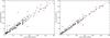 |
Fig. 6 Left panel: comparison between our inverted projected equatorial rotational velocities and the median of the catalogued ones. Right panel: comparison between our inverted projected equatorial rotational velocities and the closest of the catalogued vsini. |
Surface gravity log g
As mentioned in Sect. 1, the Hβ line is not sensitive to gravity for Teff≤ 8000 K, which applies to about 60% of our sample. For that reason, we expected that the global spectral fitting technique could derive incorrect log g values for these stars. The most reliable log g values for A-type stars are determined using photometric techniques, more precisely, from the uvbyβ calibration. The photometric values of log g are not affected by metallicity (Smalley & Dworetsky 1993). With a combination of spectroscopic and photometric techniques, the typical errors on the atmospheric parameters of a star is ±100 K for Teff and ±0.2 dex for log g (Smalley 2005). The 0.35 dex weighted average deviation and its corresponding 0.30 dex standard deviation found in the present work (Cols. 2 and 3 of Table 1), by applying Eq. (11), are justified by the use of only spectroscopic fitting technique and by the insensitivity of the Hβ line to gravity for Teff≤ 8000 K. Comparing our inverted log g to the median of the catalogued log g, we found an unweighed absolute mean signed difference of 0.40 dex with a standard deviation of about ~0.60 dex (Cols. 4 and 5 of Table 1).
Metallicity [Fe/H]
Catalogued values for metallicities exist for a small number of stars and most of them have only one determination of [Fe/H]. Statistically, our comparison with catalogued values is not reliable in this case, but the 0.15 dex that we derived using our statistical approach (Eq. (11)) is an average deviation for the derived metallicities. The standard deviation in that case is 0.25 dex (Eq. (13)). These values are identical to those derived using the unweighed differences (Cols. 4 and 5 of Table 1). Comparing with the closest catalogues values, these numbers are found to be 0.12 dex and 0.20 dex, respectively (Cols. 6 and 7 of Table 1).
Projected equatorial rotational velocity v sin i
Most of the catalogued vsini are based on the computation of the first zero of Fourier transform (FT) of Royer et al. (2002). Our spectroscopic vsini agree very well with previous findings as shown in Fig. 6, where the comparison was carried out with the median and closest catalogued values. We found a correlation coefficient of 0.96 between our inverted values and the median values from Vizier catalogues with a regression coefficient (slope) of 0.98 ± 0.02. The correlation coefficient reaches 0.988 when dealing with the closest values. By comparing one-to-one values between our inverted vsini and the median of the catalogued values, we found an absolute mean signed difference of 5.0 km s-1 and a standard deviation of 15.0 km s-1 (Cols. 4 and 5 of Table 1). In comparison with the closest values, the absolute mean signed difference is found to be 1.7 km s-1 with a standard deviation of 10.0 km s-1 (Cols. 6 and 7 of Table 1). Taking into account the spread in the catalogued values by applying Eq. (11) decreases the average deviation to ~2.0 km s-1 and the corresponding standard deviation to 9.5 km s-1 (Cols. 2 and 3 of Table 1). This result shows that the projected equatorial rotational velocities of A-type stars can be derived with a small uncertainty using PCA-inversion techniques.
5.2.1. Well-studied A stars
We also checked the deviation of our derived parameters with those of some well-studied stars. To accomplish this, we selected all of the stars that have been studied extensively by different authors using different techniques (photometric, spectroscopic, and/or interferometric). In lack of a benchmark stars list for A stars (see for instance Blanco-Cuaresma et al. 2014 for a list of FGK benchmark stars), our selection of well-studied stars is based on the number of references that we found and the number of derived values for each individual parameter for each star. In our selection, we also took stars with existing photometric determinations of Teff/log g into account. We ended up with 19 stars with more than 120 references each. The selected stars are Vega, Sirius A, HD 22484, HD 15318, HD 76644, HD 49933, HD 214994, HD 214923, HD 113139, HD 114330, HD 27819, HD 5448, HD 33256, HD 29388, HD 91480, HD 30210, HD 32301, HD 28355, and HD 222603. Considering these stars, and comparing our inverted parameters to the median of the catalogued stars, we obtain an absolute mean signed difference of 35 K with a standard deviation of 250 K for Teff, 0.18 dex with a standard deviation of 0.40 dex for log g, 0.09 dex with a standard deviation of 0.15 dex for [Fe/H], and 4.0 km s-1 with a standard deviation 9.5 km s-1 for vsini. These differences and standard deviations are shown in Cols. 8 and 9 of Table 1. The absolute mean signed differences and their corresponding standard deviations decrease when comparing with the closest catalogues values (Cols. 10 and 11 of Table 1). These calculations also show that the effective temperatures, metallicities, and projected equatorial rotational velocities of A stars can be derived with a good accuracy using PCA-inversion techniques.
6. Outliers
The outliers have been selected based on the large difference between the inverted parameters and the values retrieved from the catalogues. We also considered as outliers, and checked in detail, stars that were found to have very low metallicities. As explained in Sect. 5, gravity is usually determined with poor accuracy in spectral fitting technique for Teff≤8000 K, but we are confident that with our large wavelength range we are able to reach realistic values for these stars due to the sensitivity of the metallic lines to surface gravity (Ryabchikova et al. 2015). This is justified by the small differences that we found between the inverted and median log g (Sect. 5.2). For that reason we decided to exclude gravity as a parameter for the outliers selection.
6.1. HD 6530
Cowley et al. (1969) classified this star as A1V with no observable peculiarity. Royer et al. (2014) suspected that this star could be a binary system as the cross-correlation function has an asymmetric profile. Figure 7 shows the profile of several lines in the SOPHIE spectrum of HD 6530. All lines have flat cores. More observations are needed to confirm whether HD 6530 is a binary system or whether signatures of gravity darkening due to fast rotation seen pole-on is present in the spectrum.
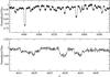 |
Fig. 7 Observed spectrum of HD 6530. Two different regions are shown in order to show the peculiar line profile that could be due to a binary system. |
6.2. HD 12446
HD 12446 has been classified as a kA2hF2mF2 star by Gray & Garrison (1989) and is considered as a normal star in Simbad. Eggleton & Tokovinin (2008) found that this star is a member of a binary system containing a A0pSi primary (V = 4.16) and an A9 secondary (V = 5.27). The contribution of an Ap star and Am star to the spectrum probably accounts for the discrepancy between the inverted parameters and those retrieved from catalogues, especially for the projected equatorial rotational velocity.
6.3. HD 16605
HD 16605, member of NGC 1039, is an A1-type star according to Renson & Manfroid (2009). The magnetic field of the star was discovered by Kudryavtsev et al. (2006) with a longitudinal component that varies from −2430 G to −840 G. Balega et al. (2012) considered this star an A1p with a peculiarity of the type SiSrCr. They also spectroscopically derived an effective temperature of 10 350 K and a vsini of 13 km s-1 close to our inverted values of 10 800 K and 14 km s-1, respectively. Their values were not found by querying Vizier and, hence, are not present in Table 2. Using interferometric data, Balega et al. (2012) discovered that HD 16605 has a companion F star, 3.1 mag fainter, with an orbital period of 680 years. The fact that HD 16605 is an Ap star with overabundances of Si, Sr, and Cr could explain the large metallicity that we derived (1.1 dex). As an A1-type star, the catalogue median temperature of 8000 K is clearly underestimated. ATLAS9 model atmospheres and the spectrum synthesis used here do not properly account for the effect of the magnetic field. The magnetic pressure is ignored in the hydrostatic equilibrium when computing the atmospheric structure in ATLAS9 and the Zeeman splitting of the line profile is not included in the line synthesis. For that reason, the PCA-inversion technique presented in this work may not be applicable for Ap stars using ATLAS9 and SYNSPEC.
6.4. HD 23479
Classified as A7V, HD 23479 was suspected to be a spectroscopic binary by Liu et al. (1991). It has a visual companion in the Tycho Catalog with separation 0.̋85, V = 9.45, and B−V = 0.54 according to Malkov et al. (2012). These authors also showed that HD 23479 is a binary system containing a A7 + F6 star. Our inverted Teff and vsini (7300 K and 2.0 km s-1) are in good agreement with previous findings (7239 K and 0.0 km s-1). This star was flagged as an outlier because of the high iron abundance (+2.0 dex). This large overabundance could be explained by two contributors in the spectrum of this star, and as a spectroscopic binary, our inverted parameters do not represent the fundamental parameters of the components of HD 23479.
6.5. HD 50405
According to McCuskey (1956), HD 50405 is classified as a A0 star in Simbad. Lefèvre et al. (2009) detected, in their preliminary work, a possible variability in HD 50405 of the δ Scuti type. By carefully inspecting the NARVAL high-resolution spectrum of HD 50405 in Fig. 8, we found a contribution of another component. This star is a member of a binary system with a component of probably a similar spectral type and should be classified as such. The variation of the radial velocity between the two components was found to be constant along the spectrum with a value close to 170 km s-1. This strengthens the hypothesis that the star is actually a binary. This star will be subject of a detailed study to better characterize the system. The presence of double lines is the reason for the discrepancies between the inverted parameters and the catalogued parameters.
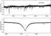 |
Fig. 8 Observed spectrum of HD 50405 around the Mg ii and Fe ii lines (upper panel) and the Hβ line (lower panel). |
6.6. HD 172271
According to Simbad, this star is classified as A1 by Renson & Manfroid (2009). Landstreet et al. (2008) detected a magnetic field of ~260 G in this star and classified it as A0pCr. In their paper, they derived a vsini of about 107 km s-1 very close to the 100 km s-1 that we found from our inversion. Landstreet et al. (2008) also derived the abundance of Cr and found an overabundance of about 2.5 dex, while Fe is about 0.5 dex overabundant. Their iron abundance is close to our inverted value of 0.4 dex. The inverted parameters of HD 172271 were rejected because it is an Ap star.
7. Discussion and conclusions
Using the PCA inversion, we have derived the effective temperature of “normal” A and Am stars with an average deviation of ~150 K with respect to the catalogued values and with a standard deviation of 500 K. We derive log g, [Fe/H] and vsini with a deviation of 0.35 dex, 0.15 dex, and 2 km s-1, respectively. Their standard deviations are 0.3 dex, 0.25 dex, and 9.5 km s-1, respectively. This assessment was carried out using an automated and objective approach that takes the large spread in the catalogued data into account.
We also derived, for the first time, the metallicity of a large number of A-type stars. The combination of vsini and [Fe/H] is a very important parameter for a first detection of the Am phenomenon. It has been shown that for the same spectral type, Am stars have lower projected equatorial rotational velocities than “normal” A-type stars and are usually slightly overabundant in iron (Gebran et al. 2008, 2010; Gebran & Monier 2008).
One could also use a learning data set based on benchmark stars with accurate stellar parameters. This could be possible with large survey calibration such as Gaia. The radial velocity spectrometer (RVS) onboard of Gaia will collect about 15 × 106 spectra during its five-year missions. The RVS will provide spectra in the CaII IR triplet region (from 8470 to 8710 Å) at a spectral resolution of ~11 000. In case of A-type stars, the RVS wavelength range contains the CaII triplet as well as N I, S I, Si I, and the strong Paschen hydrogen lines that are a good indicator of surface gravity at the temperature of A-type stars. Recio-Blanco et al. (2016), using only 490 synthetic spectra as a learning database, showed that the parameters of A-type stars can be derived with high accuracy in the RVS spectral range (see Sect. 5.2 of their paper). In their work, they compared the performance of different codes on the stellar parameters derived from the RVS spectra. We intend to test the PCA-inversion technique in a similar manner, with a much larger database, to show its efficiency at low resolution and in the RVS spectral range for not only A-type stars, but also for late- and early-type stars.
A preliminary work was published in (Farah et al. 2015), where we estimated stellar parameters of early-type stars observed in the context of the Gaia-ESO Survey (GES; Gilmore et al. 2012). This survey collects observations of faint stars (14 <V< 19) taken using the GIRAFFE/FLAMES spectrograph at a medium resolution of R ~ 25 000. Two spectral regions were used, one covering the Hδ line and one between 4400 and 4550 Å, that are similar to the wavelength range used in the present work. Although the spectral resolution is low compared to those of the SOPHIE or PolarBase spectra, we derived stellar parameters in good agreement with those recommended by the GES community.
As a conclusion, the work of Paletou et al. (2015b,c) and the present one show that the PCA-inversion method proves to be fast and efficient for inverting stellar parameters of FGK and A/Am stars and deriving effective temperatures of M dwarf stars. We built a learning database containing 2.2 × 10⁶ synthetic spectra at each resolution. For the first time, we used the power iteration algorithm to derive the eigenvectors/principal components of such a large database. The advantage of such an algorithm is that it can be used no matter the size of the database. All the synthetic data were calculated with a microturbulence velocity of 2 km s-1. This parameter, in case of 1D models, should be considered with caution, especially when attempting to model line profiles. One should modify this parameter in the learning database adopting the appropriate value for the effective temperature of the star. Gebran et al. (2014) derived the dependence of ξt on the effective temperature showing a broad maximum around 8000 K. We are working on implementing this equation in the calculations of learning databases for F-A-B stars.
Acknowledgments
This research has made use of the VizieR catalogue access tool, CDS, Strasbourg, France. The original description of the VizieR service was published in A&AS 143, 23. This research has made use of the SIMBAD database, operated at CDS, Strasbourg, France. This research has used the Polarbase, Elodie, and Sophie databases. PolarBase is operated by the OV-GSO data centre, CNRS-INSU, and Observatoire Midi–Pyrénées – Université Paul Sabatier, Toulouse, France (Paletou et al. 2015a). M.G. thanks Dr. Joe Malkoun for his valuable comments and help in the implementation of the power iteration technique. We also thank the anonymous referee for his valuable comments that helped improving this manuscript.
References
- Bailer-Jones, C. A. L., Irwin, M., & von Hippel, T. 1998, MNRAS, 298, 361 [NASA ADS] [CrossRef] [Google Scholar]
- Balega, Y. Y., Dyachenko, V. V., Maksimov, A. F., et al. 2012, Astrophys. Bull., 67, 44 [NASA ADS] [CrossRef] [Google Scholar]
- Baranne, A., Queloz, D., Mayor, M., et al. 1996, A&AS, 119, 373 [NASA ADS] [CrossRef] [EDP Sciences] [Google Scholar]
- Blanco-Cuaresma, S., Soubiran, C., Jofré, P., & Heiter, U. 2014, A&A, 566, A98 [NASA ADS] [CrossRef] [EDP Sciences] [Google Scholar]
- Borne, K. 2013, Planets, Stars and Stellar Systems, Vol. 2: Astronomical Techniques, Software and Data, 403 [Google Scholar]
- Castelli, F., & Kurucz, R. L. 2003, in Modelling of Stellar Atmospheres, Proc. IAU Symp., 210, 20 [Google Scholar]
- Catanzaro, G., & Balona, L. A. 2012, MNRAS, 421, 1222 [NASA ADS] [CrossRef] [Google Scholar]
- Code, A. D., Bless, R. C., Davis, J., & Brown, R. H. 1976, ApJ, 203, 417 [NASA ADS] [CrossRef] [Google Scholar]
- Cowley, A., Cowley, C., Jaschek, M., & Jaschek, C. 1969, AJ, 74, 375 [NASA ADS] [CrossRef] [Google Scholar]
- Demmel, J. W. 1997, Applied Numerical Linear Algebra (Philadelphia: SIAM) [Google Scholar]
- Eggleton, P. P., & Tokovinin, A. A. 2008, MNRAS, 389, 869 [NASA ADS] [CrossRef] [Google Scholar]
- Farah, W., Gebran, M., Paletou, F., & Blomme, R. 2015, Proc. SF2A, 3 http://sf2a.eu/spip/spip.php?article638 [Google Scholar]
- Gazzano, J.-C., de Laverny, P., Deleuil, M., et al. 2010, A&A, 523, A91 [NASA ADS] [CrossRef] [EDP Sciences] [Google Scholar]
- Gebran, M., & Monier, R. 2008, A&A, 483, 567 [NASA ADS] [CrossRef] [EDP Sciences] [Google Scholar]
- Gebran, M., Monier, R., & Richard, O. 2008, A&A, 479, 189 [NASA ADS] [CrossRef] [EDP Sciences] [Google Scholar]
- Gebran, M., Vick, M., Monier, R., & Fossati, L. 2010, A&A, 523, A71 [NASA ADS] [CrossRef] [EDP Sciences] [Google Scholar]
- Gebran, M., Monier, R., Royer, F., Lobel, A., & Blomme, R. 2014, Putting A Stars into Context: Evolution, Environment, and Related Stars, 193 [Google Scholar]
- Gilmore, G., Randich, S., Asplund, M., et al. 2012, The Messenger, 147, 25 [NASA ADS] [Google Scholar]
- Gray, D. F. 1992, The observation and analysis of stellar photospheres, Camb. Astrophys. Ser., 20 [Google Scholar]
- Gray, R. O., & Garrison, R. F. 1989, ApJS, 70, 623 [NASA ADS] [CrossRef] [Google Scholar]
- Grevesse, N., & Sauval, A. J. 1998, in Solar Composition and Its Evolution – From Core to Corona, Proc. ISSI Workshop, 161 [Google Scholar]
- Heiter, U., Kupka, F., van’t Veer-Menneret, C., et al. 2002, A&A, 392, 619 [NASA ADS] [CrossRef] [EDP Sciences] [Google Scholar]
- Hill, G. M., & Landstreet, J. D. 1993, A&A, 276, 142 [NASA ADS] [Google Scholar]
- Hill, G., Gulliver, A. F., & Adelman, S. J. 2010, ApJ, 712, 250 [NASA ADS] [CrossRef] [Google Scholar]
- Hubeny, I., & Lanz, T. 1992, A&A, 262, 501 [NASA ADS] [Google Scholar]
- Jolliffe, I. T. 1986, Springer Series in Statistics (Berlin: Springer) [Google Scholar]
- Kantor, J., Axelrod, T., Becla, J., et al. 2007, Astronomical Data Analysis Software and Systems XVI, 376, 3 [NASA ADS] [Google Scholar]
- Kudryavtsev, D. O., Romanyuk, I. I., Elkin, V. G., & Paunzen, E. 2006, MNRAS, 372, 1804 [Google Scholar]
- Kurucz, R. L. 1992, Rev. Mex. Astron. Astrofis., 23, 45 [Google Scholar]
- Kurucz, R. L. 2005, Mem. Soc. Astron. It. Suppl., 8, 14 [Google Scholar]
- Landstreet, J. D. 2011, A&A, 528, A132 [NASA ADS] [CrossRef] [EDP Sciences] [Google Scholar]
- Landstreet, J. D., Silaj, J., Andretta, V., et al. 2008, A&A, 481, 465 [NASA ADS] [CrossRef] [EDP Sciences] [Google Scholar]
- Lefèvre, L., Michel, E., Aerts, C., et al. 2009, Comm. Asteroseismol., 158, 189 [NASA ADS] [Google Scholar]
- Liu, T., Janes, K. A., & Bania, T. M. 1991, ApJ, 377, 141 [NASA ADS] [CrossRef] [Google Scholar]
- Malkov, O. Y., Tamazian, V. S., Docobo, J. A., & Chulkov, D. A. 2012, A&A, 546, A69 [NASA ADS] [CrossRef] [EDP Sciences] [Google Scholar]
- McCuskey, S. W. 1956, ApJS, 2, 271 [NASA ADS] [CrossRef] [Google Scholar]
- Moultaka, J., Ilovaisky, S. A., Prugniel, P., & Soubiran, C. 2004, PASP, 116, 693 [NASA ADS] [CrossRef] [Google Scholar]
- Munari, U., Zwitter, T., & Siebert, A. 2005, The Three-Dimensional Universe with Gaia, ESA SP, 576, 529 [NASA ADS] [Google Scholar]
- Paletou, F., & Zolotukhin, I. 2014, ArXiv e-prints [arXiv:1408.7026] [Google Scholar]
- Paletou, F., Glorian, J.-M., Génot, V., et al. 2015a, in SF2A-2015: Proc. Annual meeting of the French Society of Astronomy and Astrophysics, eds. F. Martins, S. Boissier, V. Buat, L. Cambrésy, & P. Petit, 37 [Google Scholar]
- Paletou, F., Böhm, T., Watson, V., & Trouilhet, J.-F. 2015b, A&A, 573, A67 [NASA ADS] [CrossRef] [EDP Sciences] [Google Scholar]
- Paletou, F., Gebran, M., Houdebine, E. R., & Watson, V. 2015c, A&A, 580, A78 [NASA ADS] [CrossRef] [EDP Sciences] [Google Scholar]
- Perryman, M. A. C., de Boer, K. S., Gilmore, G., et al. 2001, A&A, 369, 339 [NASA ADS] [CrossRef] [EDP Sciences] [Google Scholar]
- Petit, P., Louge, T., Théado, S., et al. 2014, PASP, 126, 469 [NASA ADS] [CrossRef] [Google Scholar]
- Przybilla, N., & Butler, K. 2004, ApJ, 609, 1181 [NASA ADS] [CrossRef] [Google Scholar]
- Recio-Blanco, A., de Laverny, P., Allen de Prieto, C., et al. 2016, A&A, 585, A93 [NASA ADS] [CrossRef] [EDP Sciences] [Google Scholar]
- Rees, D. E., López Ariste, A., Thatcher, J., & Semel, M. 2000, A&A, 355, 759 [NASA ADS] [Google Scholar]
- ReFiorentin, P., Bailer-Jones, C. A. L., Lee, Y. S., et al. 2007, A&A, 467, 1373 [NASA ADS] [CrossRef] [EDP Sciences] [Google Scholar]
- Renson, P., & Manfroid, J. 2009, A&A, 498, 961 [NASA ADS] [CrossRef] [EDP Sciences] [Google Scholar]
- Richer, J., Michaud, G., & Turcotte, S. 2000, ApJ, 529, 338 [NASA ADS] [CrossRef] [Google Scholar]
- Richard, O., Michaud, G., & Richer, J. 2001, ApJ, 558, 377 [NASA ADS] [CrossRef] [Google Scholar]
- Richard, O., Michaud, G., & Richer, J. 2002, ASP Conf. Proc., IAU Colloq. 185: Radial and Nonradial Pulsations as Probes of Stellar Physics, 259, 270 [NASA ADS] [Google Scholar]
- Roweis, S. 1998, in Advances in Neural Information Processing Systems (MIT Press), 626 [Google Scholar]
- Royer, F., Grenier, S., Baylac, M.-O., Gómez, A. E., & Zorec, J. 2002, A&A, 393, 897 [NASA ADS] [CrossRef] [EDP Sciences] [Google Scholar]
- Royer, F., Gebran, M., Monier, R., et al. 2014, A&A, 562, A84 [NASA ADS] [CrossRef] [EDP Sciences] [Google Scholar]
- Ryabchikova, T., Piskunov, N., & Shulyak, D. 2015, Physics and Evolution of Magnetic and Related Stars, 494, 308 [Google Scholar]
- Smalley, B. 2004, The A-Star Puzzle, IAU Symp., 224, 131 [NASA ADS] [CrossRef] [Google Scholar]
- Smalley, B. 2005, Mem. Soc. Astron. It. Suppl., 8, 130 [Google Scholar]
- Smalley, B., & Dworetsky, M. M. 1993, A&A, 271, 515 [NASA ADS] [Google Scholar]
- Steinmetz, M. 2003, GAIA Spectroscopy: Science and Technology, ASP Conf. Proc., 298, 381 [Google Scholar]
- Takeda, Y., Kawanomoto, S., & Ohishi, N. 2008, ApJ, 678, 446 [NASA ADS] [CrossRef] [Google Scholar]
- Takeda, Y., Kang, D.-I., Han, I., Lee, B.-C., & Kim, K.-M. 2009, PASJ, 61, 1165 [NASA ADS] [Google Scholar]
- Tonry, J., & Davis, M. 1979, AJ, 84, 1511 [NASA ADS] [CrossRef] [Google Scholar]
- Vick, M., Michaud, G., Richer, J., & Richard, O. 2010, A&A, 521, A62 [NASA ADS] [CrossRef] [EDP Sciences] [Google Scholar]
- York, D. G., Adelman, J., Anderson, J. E., Jr., et al. 2000, AJ, 120, 1579 [Google Scholar]
- Zahn, J.-P. 2005, EAS Pub. Ser., 17, 157 [Google Scholar]
All Tables
Average weighted deviations between our inverted parameters and catalogued values (Δw) with their respective standard deviation (σw).
All Figures
|
Fig. 1 Upper panel: continuum correction using eight iterations for the inversion of HD 97230. Only iterations 1 and 8 are shown for the sake of clarity, The initial observation is indicated with a solid line, the 1st iteration is indicated with dash-dotted line, the 8th iteration is indicated with double dash-dotted line, and the final best-fit synthetic spectrum is indicated with a dashed line. Lower panel: ratios between the re-normalized spectrum of the observation and the first neighbour best-fit synthetic spectrum for iterations 1, 2, and 8. |
| In the text | |
|
Fig. 2 First neighbour fit of synthetic spectra to the observed spectra for the four spectra of Vega, observed at different epochs, retrieved from PolarBase and SOPHIE databases. Observed spectra are shown in black and the synthetic spectra are shown in red. Part a) represents the overall spectrum, whereas part b) indicates the region sensitive to [Fe/H] and vsini. The wavelengths are in Å. Spectra were offset by arbitrary amounts. |
| In the text | |
|
Fig. 3 Comparison between our estimate of effective temperatures (•), and the values we obtained from available Vizier catalogues, for PolarBase spectra. The latter collections are represented as classical boxplots. Objects we studied are listed along the horizontal axis. The number of values found among all Vizier catalogues are presented on a horizontal line around Teff ~ 4000 K. The horizontal bar inside each box indicates the median (Q2 value), while each box extends from first quartile, Q1, to third quartile Q3. Extreme values, still within a 1.5 times the interquartile range away from either Q1 or Q3, are connected to the box with dashed lines. Outliers are denoted by a “+” symbol. |
| In the text | |
|
Fig. 4 First neighbour fit of synthetic spectra to the observed spectra. The wavelengths are in Å. Spectra were shifted up for clarity. |
| In the text | |
|
Fig. 5 Left panel: comparison between our inverted effective temperatures and the median of the catalogued effective temperatures. Right panel: comparison between our inverted effective temperatures and the closest of the catalogued effective temperatures. |
| In the text | |
|
Fig. 6 Left panel: comparison between our inverted projected equatorial rotational velocities and the median of the catalogued ones. Right panel: comparison between our inverted projected equatorial rotational velocities and the closest of the catalogued vsini. |
| In the text | |
|
Fig. 7 Observed spectrum of HD 6530. Two different regions are shown in order to show the peculiar line profile that could be due to a binary system. |
| In the text | |
|
Fig. 8 Observed spectrum of HD 50405 around the Mg ii and Fe ii lines (upper panel) and the Hβ line (lower panel). |
| In the text | |
Current usage metrics show cumulative count of Article Views (full-text article views including HTML views, PDF and ePub downloads, according to the available data) and Abstracts Views on Vision4Press platform.
Data correspond to usage on the plateform after 2015. The current usage metrics is available 48-96 hours after online publication and is updated daily on week days.
Initial download of the metrics may take a while.