| Issue |
A&A
Volume 589, May 2016
|
|
|---|---|---|
| Article Number | A53 | |
| Number of page(s) | 13 | |
| Section | Numerical methods and codes | |
| DOI | https://doi.org/10.1051/0004-6361/201527931 | |
| Published online | 13 April 2016 | |
A two-component model for fitting light curves of core-collapse supernovae
1
Department of Optics and Quantum ElectronicsUniversity of
Szeged,
6720
Szeged,
Hungary
e-mail:
This email address is being protected from spambots. You need JavaScript enabled to view it.
2
Department of Astronomy, University of Texas at
Austin, Austin,
TX,
USA
Received: 9 December 2015
Accepted: 10 February 2016
Abstract
We present an improved version of a light curve model that is able to estimate the physical properties of different types of core-collapse supernovae that have double-peaked light curves and do so in a quick and efficient way. The model is based on a two-component configuration consisting of a dense inner region and an extended low-mass envelope. Using this configuration, we estimate the initial parameters of the progenitor by fitting the shape of the quasi-bolometric light curves of 10 SNe, including Type IIP and IIb events, with model light curves. In each case we compare the fitting results with available hydrodynamic calculations and also match the derived expansion velocities with the observed ones. Furthermore, we compare our calculations with hydrodynamic models derived by the SNEC code and examine the uncertainties of the estimated physical parameters caused by the assumption of constant opacity and the inaccurate knowledge of the moment of explosion.
Key words: methods: analytical / supernovae: general
© ESO, 2016
1. Introduction
Core-collapse supernovae (CCSNe) form a heterogeneous group of supernova explosion events, but all of them are believed to arise from the death of massive stars (M> 8 M⊙). The classification of these events is based on both their spectral features and light-curve properties. Core-collapse SNe are divided into several groups: Type Ib/Ic, Type IIP, Type IIb, Type IIL, and Type IIn (Filippenko 1997). The different types of core-collapse SNe are thought to represent the explosion of stars with different progenitor properties, such as radii, ejected mass, and mass loss (e.g., Heger et al. 2003). Mass loss may be a key parameter in determining the type of the SN: stars having higher initial masses tend to lose their H-rich envelope, leading to Type IIb or Type Ib/Ic events, unlike the lower mass progenitors that produce Type IIP SNe. On the other hand, interaction with binary companion may also play an important role in determining He appearance of the explosion event (e.g., Podsiadlowski et al. 1992; Eldridge et al. 2008; Smartt et al. 2009).
Type IIP supernovae (SNe) are known as the most common among core-collapse SN events. This was recently revealed by Smith et al. (2011) based on the data from the targeted Lick Observatory Supernova Search (LOSS; Leaman et al. 2011), and also by Arcavi et al. (2010), who used data from the untargeted Palomar Transient Factory (PTF; Rau et al. 2009) survey. They probably originate in a red supergiant (RSG) progenitor star (e.g., Grassberg et al. 1971; Grassberg & Nadyozhin 1976; Chugai et al. 2007; Moriya et al. 2011). The light curves of Type IIP SNe are characterized by a plateau phase that lasts about 80–120 days (e.g., Hamuy 2003; Dessart & Hillier 2011; Arcavi et al. 2012) caused by hydrogen recombination and a quasi-exponential tail determined by the radioactive decay of 56Co (e.g., Arnett 1980; Nadyozhin 2003; Maguire et al. 2010). The Type IIb SNe are transitional objects between Type II and Ib explosions, and they show strong H and weak He features shortly after the explosion, but the H features weaken and the He lines get stronger at later phases. The weakness of the H features at late phases can be explained by considerable mass loss from the progenitor star, which causes the stripping of the outermost layer of the hydrogen envelope just before the explosion. One of the most important characteristics of the light curve of these events is the decline rate at late phases, which is governed by the radioactive decay of 56Co and the thermalization efficiency of the gamma-rays produced by the decay processes.
The collapse of the iron core generates a shock wave that propagates through the envelope of the progenitor star. Some core-collapse SNe, especially the Type IIb ones, show double-peaked light curves, where the first peak is thought to be dominated by the adiabatic cooling of the shock-heated hydrogen-rich envelope, and the second peak is powered by the radioactive decay of 56Ni and 56Co (e.g., Nakar & Piro 2014). The double-peak structure may be explained by assuming a progenitor with an extended, low-mass envelope that is ejected just before the explosion (Woosley et al. 1994). Thus the observed LC of such SNe is generally modeled by a two-component ejecta configuration: a compact dense core and a more extended, low-mass outer envelope on top of the core (Bersten et al. 2012; Kumar et al. 2013).
In this paper we use a semi-analytic light-curve model, which was originally presented by Arnett & Fu (1989) and later extended by Popov (1993), Blinnikov & Popov (1993), and Nagy et al. (2014), to describe the double-peaked light curves of several types of CCSNe. This model is able to produce a wide variety of SN light curves depending on the choice of the initial parameters, such as the ejected mass (Mej), the initial radius of the progenitor (R0), the total explosion energy (Etot), and the mass of the synthesized 56Ni (MNi), which directly determines the emitted flux at later phases.
This paper is organized as follows. In Sect. 2 we briefly describe the applied light-curve model and show the difference caused by various density profile approximations in the ejecta. In Sect. 3 we present an estimate of the average opacity from the SNEC hydrodynamic code (Morozova et al. 2015) and also examine the correlation between the model opacity and ejected mass. Section 4 presents the effect of the uncertainty of the moment of explosion on the derived model parameters. Sections 5 and 6 show the application of the two-component configuration for modeling several observed Type IIb and IIP SNe. In Sect. 7 we compare the expansion velocities derived from the model fits to the observed photospheric velocities of CCSNe. Finally, Sect. 8 summarizes the main conclusions of this paper.
2. Two-component light-curve model
In this paper we generalize the semi-analytic LC model presented by Nagy et al. (2014), which assumes a homologously expanding and spherically symmetric SN ejecta. The density structure of the ejecta is assumed to include an inner part with flat (constant) density extending to a dimensionless radius x0, and an outer part where the density decreases as an exponential or a power-law function. Thus, in a comoving coordinate frame the time-dependent density at a particular dimensionless radius (x) can be given as 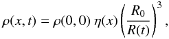 (1)where R0 is the initial radius of the progenitor, R(t) = R0 + vexpt is the radius of the expanding envelope at the given time t since explosion, vexp is the expansion velocity, ρ(0,0) is the initial density of the ejecta at the center (x = 0), and η(x) is the dimensionless density profile (see also Arnett & Fu 1989).
 |
Fig. 1 Comparison of temperature profiles applied in our code (continuous lines) to those of Blinnikov & Popov (1993) that are valid for power-law ejecta density distribution (dashed lines). The left panel shows ψ(x) of Arnett’s “radiative zero” solution, together with the BP93 profile for a n = 2 power-law index. In the right panel, the temperature profiles of our two-component models for both Type IIb and Type II-P configurations are compared to BP93 profiles having steep (n = 7) density profiles on top of the core. See text for explanation. |
The spatial structure of the density for an exponential density profile is  (2)while for the power-law density profile, it is
  (3)where a and n are small positive scalars. The initial central density of the ejecta depends on the ejected mass Mej and the progenitor radius R0 as
 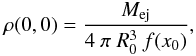 (4)where f(x0) is a geometric factor related to the density profile η(x) within the ejecta. For the exponential density profile
 ![Mathematical equation: \begin{eqnarray} f(x_0) &=&\frac{x_0^3}{3} + \frac{1}{a} \left\lbrace x_0^2 +\frac{2}{a} \left[x_0 - {\rm e}^{(x_0 - 1)}\right] \right.\nonumber\\ &&\left. + \frac{2}{a^2} \left[1-{\rm e}^{(x_0 - 1)}\right] - {\rm e}^{(x_0 - 1)} \right\rbrace, \end{eqnarray}](/articles/aa/full_html/2016/05/aa27931-15/aa27931-15-eq25.png) (5)while for power-law density distribution (Vinkó et al. 2004)
(5)while for power-law density distribution (Vinkó et al. 2004) 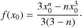 (6)The kinetic energy of a model with a given density profile and expansion velocity can be derived as
 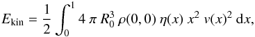 (7)where v(x) = xvexp comes from the condition of homologous expansion. Taking the form of the density profile into account, this integral can be expressed as
 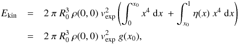 (8)where we define g(x0) as the sum of the two integrals in Eq. (8). For the exponential density profile, this is
 ![Mathematical equation: \begin{eqnarray*} g(x_0) &=& \frac{x_0^5}{5} + \frac{1}{a}\ \Bigg\lbrace x_0^4 +\frac{4}{a}\ \left[x_0^3 - {\rm e}^{(x_0 - 1)}\right] + \frac{12}{a^2}\ \left[x_0^2 - {\rm e}^{(x_0 - 1)}\right] \nonumber\\ &&+ \frac{24}{a^3}\ \left[x_0 - {\rm e}^{(x_0 - 1)}\right] + \frac{24}{a^4}\ \left[1 - {\rm e}^{(x_0 - 1)}\right] - {\rm e}^{(x_0 - 1)} \Bigg\rbrace. \end{eqnarray*}](/articles/aa/full_html/2016/05/aa27931-15/aa27931-15-eq31.png) However, for the power-law density structure, we have
However, for the power-law density structure, we have 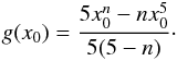 (9)Substituting Eq. (4) into Eq. (7), the expansion velocity turns out to be
 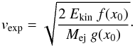 (10)We adopt the definition of vexp as the velocity of the outmost layer of the SN ejecta. This may or may not be related directly to any observable SN velocity. See Sect. 7 for a discussion of the expansion velocities in CCSNe.
In this LC model, the energy loss driven by radiation transport is treated by the diffusion approximation, and the bolometric luminosity (Lbol) is determined by the energy release due to recombination processes (Lrec) and radioactive heating (LNi) (Arnett & Fu 1989; Nagy et al. 2014). An alternative energy source, the spin-down of a magnetar (Kasen & Bildsten 2010; Inserra et al. 2013), is also built into the model, which may be useful for fitting the LC of super-luminous SNe (SLSNe). The effect of gamma-ray leakage is also taken into account as Lbol = LNi(1−exp(−Ag/t2)) + Lrec, where the Ag factor refers to the effectiveness of gamma-ray trapping (Chatzopoulos et al. 2012). It is related to the T0 parameter defined by Wheeler et al. (2015) as  .
.
In the two-component model we use two such spherically symmetric ejecta components, both having different mass, radius, energy, and density configurations. The two components have a common center, and one has much larger initial radius, but lower mass and density than the other. In the followings we refer to the bigger, less massive component as the “envelope” (or “shell”), and the more massive, smaller, denser component as the “core”. Usually, the core has higher kinetic and thermal energy than the outer envelope. This configuration is intended to mimic the structure of a red or yellow supergiant having an extended, low-density outer envelope on top of a more compact and more massive inner region. This configuration is similar to the ejecta model used by Bersten et al. (2012) for modeling the LC of the Type IIb SN 2011dh. The advantage of this two-component configuration is that it allows the separate solution of the diffusion equation in both components (see Kumar et al. 2013), if the photon diffusion time scale is much lower in the outer shell than in the core.
For Type IIb SNe, we assume that the outer envelope is H-rich, while the inner core is He-rich, both having a constant Thompson-scattering opacity. In early phases the radiation from the cooling envelope dominates the bolometric light curve, while a few days later the LC is governed by the photon diffusion from the inner core, which is centrally heated by the decay of the radioactive nickel and cobalt. The shape of the observed light curve is determined by the sum of these two processes.
Although the plateau-like LCs of Type IIP SNe can be modeled by simple semi-analytic codes (e.g., Arnett et al. 1989; Arnett & Fu 1989; Nagy et al. 2014), at very early epochs, the bolometric LC of Type IIP supernovae also show a faster declining part, which is similar to the first peak in Type IIb LCs. Thus, the two-component ejecta configuration can be a possible solution for modeling the entire LC of Type IIP SNe, but in this case the initial radii and the total energies of the two ejecta components may have the same order of magnitude. This means that the two components are not separated well, unlike in the Type IIb models. Within this context, the outer envelope may represent the outermost part of the atmosphere of the progenitor star, which has a different density profile and lower mass than the inner region. An alternative scenario is available in the literature (Moriya et al. 2011; Chugai et al. 2007). This scheme assumes a low-mass circumstellar medium (CSM) around the progenitor, which may be triggered by the mass-loss processes of the star during the RGB phase. The low-mass extended envelope might be physically associated with this CSM envelope. Indeed, some Type IIP SNe are also reported as showing the possible effects of CSM interaction in the light curves (Moriya et al. 2011) and also in the spectra (Chugai et al. 2007).
2.1. Temperature profile in the two-component model
When we take the recombination process into account, the temperature profile may play an important role during the calculation of the model LC. According to Arnett & Fu (1989), the temperature distribution within the ejecta is approximated as 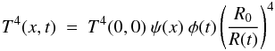 (11)where the spatial part, ψ(x), is assumed to be independent of time, and the function φ(t) represents a time-dependent scaling factor, while (R0/R(t))4 describes the adiabatic expansion of the ejecta. As in Nagy et al. (2014), we assumed Arnett’s “radiative zero” solution for the spatial profile: ψ(x) = sin(πx) / (πx) for 0 <x<xi, where xi is the comoving, dimensionless radius of the recombination front (Arnett & Fu 1989; Popov 1993). This solution is valid in a constant density ejecta. Since in our models we used a constant-density configuration for the core component (see below), this temperature profile is a good approximation for the inner regions.
This is, however, not necessarily true for the extended envelope, where we applied a monotonically decreasing density distribution having a power-law index of n = 2, starting from a dimensionless radius x0. (For the envelope the maximum ejecta radius differs from that of the core, thus, x0 is different in the core and in the envelope.) In such an ejecta, the spatial part of the temperature profile was derived self-consistently by Blinnikov & Popov (1993; BP93), and it can be approximately given as 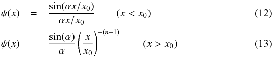 where the eigenvalue α depends on the power-law exponent as tan(α) ≈ −α/n. More details and a mathematically rigorous description can be found in Blinnikov & Popov (1993, BP93). For n = 2, we get α ≈ 2.29, which differs from the “radiative zero” value of α = π. Thus, in the envelope, the temperature in the x<x0 region is similar to but not exactly the same as the simple Arnett-solution given above. This is even more pronounced above x0, where the BP93 profile is approximately a power-law with the index of n + 1. The lefthand panel in Fig. 1 shows the comparison of the Arnett- and the BP93 ψ(x) profiles for the n = 2 power-law atmosphere. It is seen that the latter function decreases outward faster, but it does not converge to 0 at x = 1 (i.e., at maximum ejecta radius).
Despite these differences between the temperature profiles in the envelope, however, its effect on the final light curve is small. Within our modeling scheme, it only affects the outer envelope, which is thought to contain much lower mass and has much lower initial density than the core component. Thus, for numerical simplicity, we decided to apply the simple Arnett-profile for both the core and the envelope, but the estimated parameters of the envelope are somewhat affected by the choice of the temperature profile and should be treated with caution. Nevertheless, since the envelope parameters are quite weakly constrained (see below), this should not be a major concern.
The righthand panel of Fig. 1 exhibits the full normalized temperature profile (T(r) ~ ψ(r)1 / 4) as a function of ejecta radius, after joining the core and the envelope components together. The boundary between the core and the envelope is indicated by the dashed vertical line. The lefthand side of this panel shows a typical Type IIb configuration (using SN 1993J as a reference), while the righthand side displays a Type IIP model (based on SN 2013ej). It is seen that joining the two components creates a rather artificial temperature distribution that has an abrupt jump at the interface between the core and the envelope. However, the whole configuration looks more-or-less similar to a temperature profile of an ejecta having an extended envelope with quite a very steeply decreasing density profile, as illustrated by the red dashed line corresponding to a Blinnikov-Popov temperature profile having n = 7. Thus, although with an approximate and simplistic temperature distribution, our two-component configuration might mimic more-or-less the expected temperature profiles of supergiant stars having shallow inner and rapidly decreasing outer density profiles.
Moreover, according to Popov (1995), the simple Arnett-profile can be used only if the total optical depth of the envelope (τ∗ = 1 / 4βs) at a given time is higher than 1, i.e., τ∗> 1.0. In this case, β = vexp/c and  , where th and td are the hydrodynamic and the effective diffusion time scales, respectively (Arnett 1980; Popov 1995). In our models the validity of this criterion is checked at the end of the plateau phase, when the effect of recombination becomes negligible. Using the parameters derived for the modeled SNe (see below), τ∗> 4 has been found for the Type IIP SNe, while τ∗ ~ 2 have been revealed for the Type IIb models. Thus, our Type IIP models fully and the Type IIb models only marginally satisfy the condition for the photon diffusion approximation.
3. Effects of the constant opacity approximation
3.1. Calculating the average opacity from SNEC
One of the strongest simplification in semi-analytic LC models is the assumption of the constant Thompson-scattering opacity (κ), which can be defined as the average opacity of the ejecta. In this section, we approximate the average opacity via synthesized Type IIP and Type IIb light curve models.
We adopted a model star that has a mass of ~18.5 M⊙ at core collapse. The internal structure of this star was derived from a 20 M⊙ zero-age main-sequence star using the 1D stellar evolution code MESA (Paxton et al. 2013). The MESA model assumes a non-rotating, non-magnetic stellar configuration with solar metallicity and significant (10-4M⊙/ yr) mass loss. The “Dutch” wind scheme for massive stars was used to model the mass loss during the AGB and RGB phases, a scenario that combines the results from Glebbeek et al. (2009), Vink et al. (2001), and Nugis & Lamers (2000). The opacity calculation in MESA is based on the combination of opacity tables from OPAL, Ferguson et al. (2005), and Cassisi et al. (2007).
The evolution of the model star was calculated by MESA until core collapse, and this original model was used for further calculations in producing a Type IIP SN light curve. Moreover, we also built a second model for studying the light curve of Type IIb SN. To estimate the progenitor of a Type IIb SN, most of the outer H-rich envelope of the original MESA model was removed manually, so that only an envelope mass remained of ~1 M⊙. The subsequent hydrodynamic evolutions were followed by SNEC, which is a 1D Lagrangian supernova explosion code (Morozova et al. 2015). SNEC solves the hydrodynamics and diffusion radiation transport in the expanding envelopes of CCSNe, taking recombination effects and the decay of radioactive nickel into account. During the calculations the “thermal bomb” explosion scheme was used, in which the total energy of the explosion is injected into the model with an exponential decline both in time and in mass coordinate. The SNEC code calculates the opacity in each grid point of the model from Rosseland mean opacity tables for different chemical compositions, temperatures, and densities. During this process an opacity minimum was also considered by the code. In our simulations this opacity edge was 0.24 for the pure metal and 0.01 cm2/ g for the solar composition envelope (Bersten et al. 2011). Thus, in SNEC the opacity at each time and grid point is chosen as the maximum value between the calculated Rosseland mean opacity and the opacity edge for the corresponding composition.
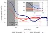 |
Fig. 2 Dependence of κ(Mph) on the time for Type IIP (blue) and Type IIb (red) SNEC model. |
To estimate the average opacity for Types IIP and IIb SNe, the original SNEC opacity output file was used. At a given time we defined κ(Mph) by integrating the opacity from the mass coordinate of the neutron star (M0 = 1.34 M⊙) up to the mass coordinate of the photosphere (Mph) as  (14)Considering that our semi-analytic model uses the same opacity when calculating the entire light curve, we defined the average opacity (
 ) by integrating κ(Mph) from several day after the shock breakout (t0) up to tend as
  (15)Figure 2. shows the dependence of κ(Mph) on the time. To receive comparable results with our two-component estimates, we separately calculated the average opacities for both the early cooling phase and the photospheric phase. In the cooling phase, t0 = 5 days, while tend was chosen as the approximate termination of the cooling phase, when the opacity drops rapidly, which was 9 days for the Type IIb model and 13 days for the Type IIP model. For the photospheric phase, t0 was defined to be equal to tend of the cooling phase, and we integrated up to the end of the nebular phase. Vertical gray lines in Fig. 2. represent these time boundaries for both Types IIb and IIP SNe. Horizontal lines indicate the different values as the average opacities of different phases and models. It can be seen that in the cooling phase, is ~0.4 cm2/g for a Type IIP SN with a massive H-rich ejecta. However, the average opacity decreases to ~0.3 cm2/ g for a Type IIb, which corresponds to a star that lost most of its H-rich envelope. In contrast, during the later phase, the average opacity of Types IIP and IIb is considerably similar, having a value of ~0.2 cm2/ g.
Model parameters for the synthetic LCs.
The constant Thompson-scattering opacity is not an adequate approximation either in early or late phases because of the rapidly changing opacities, but the calculated average opacities show reasonably good agreement with previous studies (e.g., Nakar & Sari 2010; Huang et al. 2015), where  cm2/ g was used for modeling the LCs of Type IIP SNe. Thus, in the following analysis we use the average opacities (
 cm2/ g and
  cm2/ g) from SNEC to approximate κ in the shell models of Types IIb and IIP SNe, respectively. To estimate κ for the core model we take the derived expansions velocities and the values form SNEC into account. Because the range of the varying κ values is narrower for the Type IIb than for the Type IIP configuration (see Fig. 2), then for Type IIb SNe we use κ = 0.2cm2/ g, while for Type IIP SNe κ ≈ 0.2 ± 0.1cm2/ g was chosen.
3.2. Correlation between the opacity and ejected mass
In this section we examine the effect of the constant opacity approximation, which may play an important role in analysing the fitting results, via a synthesized Type IIP light curve. In this case we use the Type IIP SNEC model discussed above (Sect. 3.1). The SNEC model light curve is compared with the light curves calculated by the semi-analytic code. Two models were computed with the latter: in Model A we used exactly the same physical parameters as in the SNEC model, but varied κ to get the best match between the two LCs. In Model B we applied κ = 0.2cm2/ g, similar to the average opacity of the SNEC model, but tweaked the other parameters until a reasonable match between the data and the model LC was found.
The parameters of the hydrodynamic model and from the semi-analytic LC models are summarized in Table 1. Even though the opacities are really different in the two models, both light curves show an acceptable match with the SNEC light curve (Fig. 3). These results represent the well-known issue that the analytic codes having constant Thompson-scattering opacity usually predict lower ejected masses than hydrodynamic calculations (e.g., Utrobin & Chugai 2009; Smartt et al. 2009). This situation is probably due to the incorrect assumption of constant opacity as well as the reduced dimension in the hydrodynamic simulations. In contrast, to get the same ejected mass in both the hydrodynamic and analytic calculations, an extremely low Thompson-scattering opacity is needed. This low opacity value may be a hint of a dominance of metals over H, which looks difficult to explain in the outer region of the H-rich ejecta.
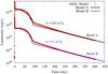 |
Fig. 3 Comparison of the bolometric light curve from SNEC (red) with the semi-analytic LCs. Models A (black) and B (blue) represent the best LC fit with low and high opacity, respectively (Table 1). The LC of Model A was shifted vertically for better visibility. |
Furthermore, to explain the possible reason for the previously mentioned ejected mass problem, we suspect that this effect is due to parameter correlation (Nagy et al. 2014). As seen in Table 1 only two parameters change drastically in the models, which suggests that the correlation between κ and Mej may play a major role in solving this problem.
To examine the effect of this correlation, we used the available hydrodynamic and analytic model parameters (R0,Mej,Ekin) of SN 1987A (see the details in Sect. 6). SN 1987A was chosen because this object is the best-studied SN ever, thus, several different model calculations are available in the literature. To estimate the opacity of these different models, we took the parameters from each published SN 1987A model, fixed them “as-is”, and fit the LC with our code while tweaking only the values of κ. The final results can be seen in Fig. 4, where each red dot represents one of the applied models. It is seen that Mej and κ-1 are strongly correlated parameters.
To illustrate a quantitative measure of the correlation we calculate the correlation coefficient as 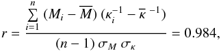 (16)where σM, σκ, and
  ,
,  are the standard deviations and the mean values of Mej and κ-1, respectively. Because r is close to 1 the ejected mass and opacity are highly correlated, which cause significant uncertainty in determining these parameters. Clearly, neither Mej nor κ can be reliably inferred from these LC models, only their product, Mej·κ, is constrained (see also Wheeler et al. 2015)
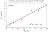 |
Fig. 4 Correlation between the opacity and the ejected mass for SN 1987A models. |
4. Effect of the uncertainty of the explosion time on the estimated parameters
When pre-explosion observations of the SN site are not available, the explosion time of the supernova can be rather uncertain. Determining the moment of first light of a supernova explosion is very important, because the shape of the rising part of the light curve depends critically on the exact date of the explosion. The physical parameters inferred from such a light curve may suffer from large systematic errors.
This effect can be even more significant in the case of SNe with extended envelopes. To estimate the uncertainty of model parameters due to the unknown date of explosion, we fit the bolometric light curve of a Type IIb (Fig. 5) and a Type IIP (Fig. 6) SN assuming different explosion dates. For these calculations we used the two-component configuration described in Sect. 2.
It is apparent from Tables 2 and 3 that for Type IIP SNe an uncertainty of about seven days in the explosion date generates moderate (5–10%) relative errors in the derived masses of the inner core (Mcore) and the outer envelope (Mshell), and the initial radius of the core (Rcore). For Type IIb SNe only MNi and the total energy of the outer envelope (Eshell) show similar uncertainties. In this case the uncertainty of the derived Mshell, Rcore and Mcore may increase up to about 50%, 40%, and 20%, respectively.
Effect of the uncertainty of the explosion time on the fit parameters for a Type IIb SN (based on the LC of SN 1993J).
Effect of the uncertainty of the explosion time on the fit parameters for a Type IIP SN (based on the LC of SN 2004et).
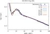 |
Fig. 5 Comparison of the bolometric light curve of the Type IIb SN 1993J (dots) with model LCs calculated with different explosion dates (lines). |
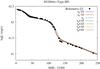 |
Fig. 6 Comparison of the bolometric light curve of the Type IIP SN 2004et (dots) with model LCs calculated with different explosion dates (lines). |
5. Model fits to Type IIb supernovae
In the following sections we apply the two-component LC model for real SNe, both Types IIb and IIP. We use the bolometric light curves of the observed SNe, assembled in a similar way to our previous paper (Nagy et al. 2014), and compare them with model light curves computed from the two-component model detailed above. Formal χ2-fitting was not performed, as the strong correlation between the parameters would make such a fit ill-constrained (see, e.g., Nagy et al. 2014). Instead, the model parameters were varied manually until reasonable agreement between the data and the model was found.
To estimate the physical properties of Type IIb SNe, we fit the light curves of two well-observed events, SN 1993J and SN 2011fu. SN 1993J was discovered in NGC 3031 (M81) on 1993 March 28.9 UT by F. Garcia (Ripero 1993). UBVRI photometry was presented by Richmond et al. (1994), who determined the moment of explosion as JD 2 449 073. SN 2011fu was discovered in a spiral galaxy UGC 1626 by F. Ciabattari and E. Mazzoni (Ciabattari et al. 2011) on 2011 September 21.04 UT. The estimated explosion date is 2011 September 18.0 (JD 2 455 822.5).
To reach better agreement with spectroscopic observations, a constant density profile was chosen in the inner core, while we used a power-law density structure (n = 2) in the outer envelope. The inner boundary (x0) of the density profile was set as  and
and  . We used κ = 0.2cm2/ g for the inner, H-poor core and κ = 0.3cm2/ g for the H-He outer envelope, which are consistent with the estimated average opacities from SNEC Type IIb model.
Owing to their lower ejected masses, the gamma-ray leakage may be significant in Type IIb SNe. Typical Ag values for these events are between 103 and 104day2. The other parameters of the best fit-by-eye models are summarized in Table 4, and the LCs are plotted in Fig. 7. From these results it can be seen that the mass of the He-rich core is ~1 M⊙, while the extended envelope contains ~0.1 M⊙, although the latter depends on the chosen value of x0 in the envelope, which is poorly constrained. Using x0 ~ 0.1 instead of 0.4 in the envelope would require somewhat higher energies and an order-of-magnitude less mass (~0.01 M⊙) to fit the initial peak.
Model parameters of Type IIb SNe.
5.1. Comparison with other models
For the examined Type IIb SNe, the physical parameters of both the envelope and the core were determined by several authors. Here we compare all of the available parameters with the values determined by the two-component LC fitting, keeping the same terminology for the parameters from the two-component models that was used in Sect. 4. The only exception is that Ecore refers to the kinetic energy of the core component.
The physical properties of SN 1993J were calculated by several LC modeling codes (Shigeyama et al. 1994; Utrobin 1994; Woosley et al. 1994; Young et al. 1995; Blinnikov et al. 1998). First, the physical properties of this explosion were determined by a hydrodynamic calculation of Shigeyama et al. (1994) as Rshell = (1.7−2.5) × 1013 cm, Ecore = 1.0–1.2 foe, while the mass of the extended envelope is below ~0.9 M⊙. The fundamental parameters of SN 1993J were also inferred by Utrobin (1994), who found that the radius of the progenitor was ~3.2 × 1012 cm, the ejected mass was ~2.4 M⊙, the nickel mass was ~0.06 M⊙, and the energy of the explosion was ~1.6 foe.
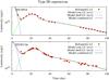 |
Fig. 7 Comparison of the bolometric light curves of Type IIb SNe (dots) with the best two-component model fits. The green and blue curves represent the contribution from He-rich core and the extended H-envelope, respectively, while the black lines show the combined LCs. |
Another scenario was modeled by the Kepler stellar evolution and hydrodynamic code based on the assumption that the progenitor of SN 1993J lost its outer H envelope because of mass transfer to a binary companion (Woosley et al. 1994). At the time of the explosion, the H envelope mass was 0.2 ± 0.05 M⊙ and the radius of the star was (4 ± 1) × 1013 cm. In this model 0.07 ± 0.01 M⊙ of 56Ni was produced during the explosion, and the ejected mass was found to be about 1.2 M⊙.
The radius of the progenitor star was estimated by Young et al. (1995) as Rshell = (2−4) × 1013 cm, while the nickel mass was found to be MNi ~ 0.1 M⊙. The ejected mass settled in the range of 1.9–3.5 M⊙. Young et al. (1995) used a H-rich atmosphere with Mshell ~ 0.1–0.5 M⊙ and Rshell ~ 1013 cm to represent the extended envelope due to the mass-loss of the progenitor just before the explosion.
The explosion of SN 1993J was also calculated with both STELLA and EDDINGTON hydrodynamic codes (Blinnikov et al. 1998). In these models 0.073 M⊙ of 56Ni was found, and 1.55 M⊙ mass was ejected with Ecore ~ 1.2 foe. Although these four calculations applied different scenarios, the obtained results are in the same parameter range and also show a good agreement with our model parameters, except for the kinetic energy (Table 5), which is usually overestimated by the semi-analytic LC fitting codes.
Model parameters for SN 1993J.
A hydrodynamic calculation for SN 2011fu was presented by Morales-Garofforo et al. (2015), assuming Rshell = 3.13 × 1013 cm, Mcore = 3.5 M⊙, Ecore = 1.3 foe, and MNi = 0.15 M⊙. The significant differences between these values and our estimates are probably due to using different distances and extinctions during the calculation of the bolometric light curve. Nonetheless, our approximate parameters are in the same order-of-magnitude as the hydrodynamic results (Table 6).
The light curve of SN 2011fu was also fit by Kumar et al. (2013) with the analytic model of Arnett & Fu (1989). They derived Rcore = 2 × 1011 cm, Mcore = 1.1 M⊙, MNi = 0.21 M⊙, and Ecore = 2.4 foe for the inner He core, while for the outer hydrogen envelope Rshell = 1013 cm, Mshell = 0.1 M⊙, and Eshell = 0.25 foe were found. These estimated values are in good agreement with our results, which is expected because both models apply similar physical modeling schemes. The minor differences in the envelope parameters are due to the differences between the adopted density profiles, because Kumar et al. (2013) use an exponential profile (a = 1) against our constant density model. We also tested the application of the exponential density profile, but the shape of the generated LC showed better agreement with the observed data in the constant density model, which is in accord with the results of Arnett & Fu (1989).
Model parameters for SN 2011fu.
6. Model fits to Type IIP supernovae
To derive the model parameters of Type IIP SN, we fit the LCs of SNe 1987A, 2003hn, 2004et, 2005cs, 2009N, 2012A, 2012aw, and 2013ej. Table 12 shows the observational properties of these events.
While fitting these SNe, we used a constant density profile for the inner core, while the outer H-rich envelope has a power-law density distribution. The constant-density approximation was found to work surprisingly well for fitting the plateau phase of Type IIP SNe except for the early cooling phase (Arnett & Fu 1989; Nagy et al. 2014).
The power-law density profile with n = 2 is an acceptable choice if we assume a steady stellar wind, similar to Moriya et al. (2011). In the outer shell the energy input from recombination was neglected because of the low envelope mass and rapid cooling in this region. However, the effect of the recombination is important in the inner core, because recombination is responsible for the appearance of the entire plateau phase. After the plateau phase, the LC follows the time-dependence of the decay of radioactive cobalt. In most cases gamma-ray leakage was found to be negligible. The two exceptions are SN 1987A and 2013ej, where the effect of gamma-ray escape was taken into account by setting Ag ~ 2.7 × 10⁵ and 3 × 10⁴ day2, respectively. For SN 1987A, the gamma-ray leakage was also examined by Popov (1992). In that study the characteristic time scale of the gamma-rays (T0) was 500–650 days, which shows reasonably good agreement with our result of  days.
days.
Model parameters of Type IIP SNe.
The best model fits for Type IIP supernovae are summarized in Table 7, and the LCs are plotted in Figs. 8–11. It can be seen that the masses of the inner region are about 7–20 M⊙, while the masses of the outer envelope are less than 1 M⊙. The total supernova explosion energies show a huge diversity, but its reality is questionable because it may be simply due to the strong correlation between the explosion energy, the ejected mass, and the progenitor radius (see, e.g., Nagy et al. 2014).
6.1. Comparison with other models
6.1.1. Normal Type IIP SNe
For Type IIP SNe only the core parameters were available in the literature. In this section, we therefore only use the parameters for this inner region to compare with those from other models. For SN 2004et, 2005cs, 2009N, 2012A, and 2012aw, the comparison between the results of our semi-analytical light curve model and the parameters of other hydrodynamic calculations was already presented in a previous paper (Nagy et al. 2014). For SN 2003hn, neither hydrodynamic calculations nor analytic models are available in the literature at present.
The radius of the progenitor star of SN 2013ej was found to be in the range of (2.8−4.2) × 1013 cm with a simple analytic function by Valenti et al. (2014). Fraser et al. (2014) estimated the progenitor in the mass range of 8–15.5 M⊙ from the luminosity on the pre-explosion images. Hydrodynamic calculations for SN 2013ej were published by Huang et al. (2015), who assumed a 56Ni mass of 0.02 ± 0.01 M⊙. Their model was computed by semi-analytic and radiation-hydrodynamical simulation as well, which yields a total energy of (0.7−2.1) × 1051 erg, an initial radius of (1.6–4.2) ×1013 cm, and an envelope mass of 10.4–10.6 M⊙. More recently, another semi-analytical model calculations were given by Bose et al. (2015) and resulted in Mej = 12 ± 3 M⊙, R0 = (3.1 ± 0.8) × 1013 cm, Etot ~ 2.3 foe, and MNi = 0.02 ± 0.002 M⊙. These parameters are very similar to our results listed in Table 8.
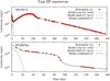 |
Fig. 8 Comparison of the bolometric light curves of Type IIP SNe (dots) with the best two-component model fits. The green and blue curves represent the contribution from the inner ejecta and the extended H envelope, respectively, while the black lines show the combined LCs. |
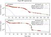 |
Fig. 9 Comparison of the bolometric light curves of Type IIP SNe (dots) with the best two-component model fits. The green and blue curves represent the contribution from the inner ejecta and the extended H envelope, respectively, while the black lines show the combined LCs. |
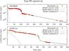 |
Fig. 10 Comparison of the bolometric light curves of Type IIP SNe (dots) with the best two-component model fits. The green and blue curves represent the contribution from the inner ejecta and the extended H envelope, respectively, while the black lines show the combined LCs. |
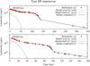 |
Fig. 11 Comparison of the bolometric light curves of Type IIP SNe (dots) with the best two-component model fits. The green and blue curves represent the contribution from He-rich core and the extended H envelope, respectively, while the black lines show the combined LCs. |
Model parameters for SN 2013ej.
6.1.2. SN 1987A, a peculiar Type IIP SN
SN 1987A was a peculiar Type IIP explosion event. The progenitor of SN 1987A was a blue supergiant star (BSG), named Sk – 69 202 (for a review, see, e.g., Arnett et al. 1989). The BSG progenitor indicates that the mass-loss was significant during the stellar evolution. Thus, in this case we assume that our shell model refers to a mass-loss event shortly before the supernova explosion, which may create a low-mass circumstellar medium (CSM) around the progenitor. For fitting SN 1987A, we therefore only used the estimated parameters of the core configuration to compare with other models.
The fundamental quantities of SN 1987A were calculated with numerous different models by several authors (Arnett & Fu 1989; Blinnikov et al. 2000; Nomoto et al. 1987; Shigeyama et al. 1987; Utrobin & Chugai 2005). The LC of this event was analyzed by Blinnikov et al. (2000) with the hydrodynamic code STELLA. That calculation assumed that the ejected mass was 14.7 M⊙, the kinetic energy was 1.1 ± 0.3 foe, and the radius of the progenitor star was about 3.4 × 1012 cm. The hydrodynamic calculation of Shigeyama et al. (1987) estimated that the radius of the progenitor star should have been about (1−3) × 1012 cm. In that publication an ejected mass of 7–10 M⊙ and an explosion energy of 2–3 foe was found.
Another hydrodynamic model was presented by Nomoto et al. (1987), which predicted 11.3 M⊙ for ejected mass, 0.07 M⊙ for the initial nickel mass, and 1.5 foe for the explosion energy. The LC of SN 1987A was analyzed by Utrobin & Chugai (2005), and their hydrodynamic model presents an ejected mass of 18 M⊙, a kinetic energy of 1.5 foe, a nickel mass of 0.077 M⊙, and a radius of 2.44 × 1012 cm. The physical properties of this supernova were also calculated by Arnett & Fu (1989) with the values of R0 = 1.05 × 1012 cm, Mej = 7.5 M⊙, Etot ≈ 1.5 foe, and MNi = 0.075 ± 0.015 M⊙. The fundamental parameters of SN 1987A were inferred by Imshennik & Popov (1992). They found that the radius of the progenitor was (1.8−2.8) × 1012 cm, the kinetic energy was 1.05–1.2 foe, the ejected mass was 15.0 M⊙, and the nickel mass was 0.071–0.078 M⊙. The comparison of all of these parameters with the ones from our LC fitting code can be found in Table 9.
From Table 9 it is seen that the numerous efforts for modeling the LC of SN 1987A led to very different physical parameters. This is especially true for the ejected mass, where a factor of 2 disagreement between the results from the early and modern hydrodynamic codes can be found. The ejected mass from our semi-analytic code, as well as the other parameters, are consistent with these hydrodynamic results. It is true that the semi-analytic code tend to predict somewhat lower ejected masses than some of the modern hydrocodes, but the difference is not higher than the differences between the results from various hydrodynamic calculations.
Although some major differences can be noticed between the published results (especially in Mej), the calculated parameters are within the same order of magnitude, and our estimates are entirely consistent with these parameter ranges. However, it should be kept in mind that in analytic models, which use the constant opacity approximation, the correlation between κ and Mej (Sect. 3.2) has a significant effect on the estimated Mej. Thus, in these models the ejected mass may only be constrained within a factor of two, if the assumed opacity is chosen between 0.1–0.3 cm2/g.
In the last row of Table 9, we show the mean light curve time scales, which is equal to the effective diffusion time scale,  days (Arnett 1980; Arnett et al. 1989), as inferred from the parameters of the different models (assuming κ ~ 0.2 cm2 g-1 for those that were not computed with constant opacity). This quantity is roughly proportional to the rise time to the LC peak (or the length of the plateau in Type IIP SNe) in the constant-density model. Since at least half of the models (S87, N87, B00, UC05) listed in Table 9 were not computed with the constant density approximation, this parameter is less applicable to those models, but generally it gives an good estimate of the relative peak times of the different models.
Model parameters for SN 1987A.
It is interesting that the models predicting more ejecta mass (Mej> 10 M⊙) all have td> 70 days, while the models with less massive ejecta consistently have peak times less than 70 days. Although for models with recombination taken into account, the actual LC peak time is somewhat longer than td (e.g., Arnett & Fu 1989), it is true that the models having longer td tend to show later peaks than the models with shorter td. Comparing the td values in Table 9 with the observed peak time of SN 1987A (td ~ 90 days, Fig. 8 upper panel), it is seen that for the models with lower masses (Mej< 10 M⊙), the inferred td parameters are consistent with the observed peak time.
Concerning the more massive models, the AF89-2 model (Mej = 15 M⊙, td = 91 d) is still more-or-less consistent with the observed LC peak, but the other three models (IP92, B00, UC05) tend to predict longer peak times than observed. This may not be surprising as far as the B00 and UC05 models are concerned, because those are radiative hydrodynamical models, for which the simple analytic estimate from the constant density model may not be applicable. However, the model of IP92 (Imshennik & Popov 1992) is also a semi-analytic model that uses similar approximations to ours here. Thus, it is not clear why this model is able to fit the observed peak of the LC of SN 1987A, while it has the longest predicted td among all models listed in Table 9. When compared with the AF89-2 model (Arnett & Fu 1989), which also has Mej = 15M⊙, it is seen that the latter has a factor of two higher kinetic energy than the IP92 model. Since higher Ekin causes the computed LC to peak earlier, the AF89-2 model with higher Ekin looks more plausible for fitting SN 1987A than the IP92 model.
It is concluded that the cause of the wide range of the predicted physical parameters listed in Table 10, in addition to the already discussed issues such as the constant opacity approximation and the opacity-mass correlation, is supposedly the strong correlations between practically all parameters involved in the LC modeling (e.g., Arnett & Fu 1989; Imshennik & Popov 1992; Nagy et al. 2014). If one, for example, assumes Mej ~ 15M⊙ ejecta mass, it is possible to find, for example, a kinetic energy that is physically realistic, and the model gives a good fit to the observed LC. The same is true for Mej< 10 M⊙, which needs lower Ekin, but is still in the ballpark, to get almost the same fitting. This is clearly a caveat of SN LC modeling, which should be kept in mind when interpreting the SN parameters inferred from pure LC fits.
7. Expansion velocity of CCSNe
An additional test of the LC models can be made via the comparison of the expansion velocities derived from the best-fitting LC models with the observed ones. We apply Eq. (11) to calculations of the expansion velocities of the SNe under study, and these values can be compared with the available velocities from spectroscopic measurements collected from literature. Since the expansion velocity (the maximum velocity in the applied semi-analytic model) cannot be measured directly, we use the observed photospheric velocities (vph) from early and late-time spectra as a proxy for the expansion velocities (see also Wheeler et al. 2015).
As a first approximation, we compare the expansion velocities of the envelope (vshell) with the earliest vph values, when the photosphere is likely in the outer envelope (see, e.g., Moriya et al. 2011). For the core expansion velocities (vcore), we use the late-phase vph values measured around the middle of the plateau phase. Tables 10 and 11 list these data for the envelope and the core, respectively.
Velocities of the outer envelope of the modeled SNe.
Velocities of the inner ejecta of the modeled SNe.
The explosion velocities derived from LC modeling are always somewhat uncertain because of the correlation between the ejected mass and the kinetic energy (see, e.g., Nagy et al. 2014). This may result in significant systematic offsets in the model velocities. Thus, we are only able to estimate the expansion velocity within a factor of ~2. Considering these circumstances, the range of the observed velocities in Tables 10 and 11 are in reasonable agreement with our model values.
Observational properties of Type IIP SNe.
We also check the correlation between vcore and vshell for both Type IIb and Type IIP SNe. As Fig. 12 shows, these two types of explosion events appear to be separated in velocity space. Type IIb SNe have higher velocities in both regions, while for Type IIP SNe only vshell may reach higher values. The differences in vcore can be explained by the difference between the fitting parameters, especially Mej and Ekin. Because the kinetic energies are in the same order of magnitude, while the ejected masses for Type IIP-s are ten times higher than for Type IIb-s, the inferred velocities for the latter are lower, in accord with simple physical expectations.
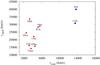 |
Fig. 12 Expansion velocities of Type IIb (blue squares) and Type IIP (red dots) supernovae. |
8. Discussion and conclusions
We have shown above that for Type IIP SNe, a two-component ejecta configuration can be appropriate to model a double-peaked light curve with a semi-analytic diffusion-recombination code. This ejecta configuration is similar to the one used for Type IIb SNe, when assuming an inner, denser core and a hydrogen-dominated outer envelope, although for Type IIb-s the envelope is much more extended than the core, unlike in Type IIP models.
There are a number of caveats in the simple diffusion-recombination model applied in this paper, such as the assumption of constant opacity in the ejecta, which naturally limits the accuracy of the derived physical parameters. Although the Thompson-scattering opacity approximation simplifies the equations, the used opacity loses its physical meaning and only becomes a fitting parameter. But the average opacities from the SNEC hydrodynamic model show adequate agreement with the frequently used opacities in literature and also with our applied κ-s. Another limitation is the uncertainty of the explosion date, which may cause 5–50% relative errors in the derived physical parameters. Despite these issues, by using simple semi-analytic models, one can estimate the initial parameters of the progenitor and the SN with an order-of-magnitude accuracy.
The final results in Sects. 5 and 6 show that Type IIP SNe have the most extended envelopes having initial radii of ~1013 cm, which is in good agreement with the radii of their presumed RSG progenitors. For these events the ejected mass of the inner region (Mcore) is about an order-of-magnitude higher than that of Type IIb SNe, which is consistent with the different physical state of their progenitors (e.g., Woosley et al. 1994; Heger et al. 2003).
In the diffusion approximation, it is important that the contributions from the two different components should be well separated. To fulfill this requirement, the diffusion time scale of the photons in the outer envelope must be much lower than that of the inner core. If this is so, the first LC peak can be explained as mostly due to the adiabatic cooling of the shock-heated H-rich envelope, where there is no energy input other than the thermal energy deposited by the initial shock wave. Thus, in very early phases, the contribution of the outer envelope dominates the luminosity. In contrast, the second LC peak is powered by radioactive decay of 56Co and the recombination of H. The energy input from these mechanisms only diffuses through the inner core before escaping as observable radiation, because in later epochs the outer envelope had already become strongly diluted, thus its effect on the light curve is negligible (Fig. 7).
From the model parameters presented in Tables 4 and 7, the effective diffusion time scale td can be inferred, which depends weakly on the density profile. For the inner core this parameter also represents the rise time and the LC width of Types IIb and IIP SNe, respectively. The typical calculated td values for Type IIP SNe are ~80–100 days, while for Type IIb they are ~20 days, which are in reasonable agreement with visually specified LC properties. Also, it can be shown that td in the core is at least two times higher than in the envelope for both Type IIP and Type IIb compositions. Thus, the two-component models given in Tables 4 and 7 are consistent with the assumption that the photon diffusion equations in the two components can be solved separately.
The Type IIP models, however, may not be entirely self-consistent, because in those cases the radius of the envelope is only two times higher than that of the core. In this case neglecting the effect of the radioactive heating in the outer envelope may not be fully justifiable. This means that the inferred envelope parameters in Table 7 are much more uncertain than the parameters of the core. In spite of this uncertainty, the envelope parameters occupy nearly the same regime as the CSM masses in the hybrid ejecta+CSM models calculated by Moriya et al. (2011). As far as the Type IIb models are concerned, the parameters in Table 4 are also in good agreement with the results by Nakar & Piro (2014), who estimate the envelope masses and the maximum radii of the core in stripped-envelope SNe.
The two-component semi-analytic model presented in this paper may be a useful tool for deriving order-of-magnitude estimates for the basic parameters of Types IIP and IIb SNe, which can be used to narrow the parameter regime in more detailed simulations. The model can predict reasonable parameters for both the inner core and the outer envelope. It can fit the entire LC starting from shortly after shock breakout throughout the end of the plateau and extending into the nebular phase.
An obvious advantage of the semi-analytic code with respect to the more computationally intense hydrodynamic codes is the execution time, which is about two minutes on a Core-i7 CPU, compared to about the ten hours needed to complete a model LC with SNEC (not to mention the more sophisticated hydrocodes that may require orders of magnitude longer time on supercomputers).
However, it should be kept in mind that some of the parameters of the semi-analytic code, such as κ, Mej, and Ekin, are correlated, thus, only their combinations are constrained by the data. Moreover, the constant κ opacity may not have the correct physical meaning, thus it should only be considered as a fitting parameter rather than a true representation of the “true” opacity in the SN atmosphere. With this limitation, the results from the two-component LC model are consistent with current state-of-the-art calculations for Type II SNe, so the estimated fitting parameters can be used for preliminary studies prior to more complicated hydrodynamic calculations.
The source code of the program applied for calculating the semi-analytic models in this paper is available online1.
Acknowledgments
We are indebted to an anonymous referee, who provided very useful comments and suggestions from which we have indeed learned a lot, and which led to significant improvement of this paper. This work has been supported by Hungarian OTKA Grant NN 107637 (PI Vinko).
References
- Arcavi, I., Gal-Yam, A., Kasliwal, M. M., et al. 2010, ApJ, 721, 777 [NASA ADS] [CrossRef] [Google Scholar]
- Arcavi, I., Gal-Yam, A., Cenko, S. B., et al. 2012, ApJ, 756, 30 [Google Scholar]
- Arnett, W. D. 1980, ApJ, 237, 541 [Google Scholar]
- Arnett, W. D., & Fu, A. 1989, ApJ, 340, 396 [NASA ADS] [CrossRef] [Google Scholar]
- Arnett, W. D., Bahcall, J. N., Kirshner, R. P., & Woosley, E. S. 1989, ARA&A, 27, 629 [NASA ADS] [CrossRef] [Google Scholar]
- Bartel, N., Bietenholz, M. F., Rupen, M. P., et al. 2002, ApJ, 581, 404 [NASA ADS] [CrossRef] [Google Scholar]
- Bersten, M. C., Benvenuto, O. G., & Hamuy, M. 2011, ApJ, 729, 61 [NASA ADS] [CrossRef] [Google Scholar]
- Bersten, M. C., Benvenuto, O. G., Nomoto, K., et al. 2012, ApJ, 757, 31 [NASA ADS] [CrossRef] [Google Scholar]
- Bessell, M. S., Castelli, F., & Plez, B. 1998, A&A, 333, 231 [NASA ADS] [Google Scholar]
- Blinnikov, S., & Popov, D. V. 1993, A&A, 274, 775 [NASA ADS] [Google Scholar]
- Blinnikov, S. I., Eastman, R., Bartunov, O. S., et al. 1998, ApJ, 496, 454 [NASA ADS] [CrossRef] [Google Scholar]
- Blinnikov, S., Lundqvist, P., Bartunov, O., et al. 2000, ApJ, 532, 1132 [NASA ADS] [CrossRef] [Google Scholar]
- Bose, S., Kumar, B., Sutaria, F., et al. 2013, MNRAS, 483, 187 [Google Scholar]
- Bose, S., Sutaria, F., Kumar, B., et al. 2015, ApJ, 806, 160 [NASA ADS] [CrossRef] [Google Scholar]
- Cassisi, S., Potekhin, A. Y., Pietrinferni, A., et al. 2007, ApJ, 661, 1094 [NASA ADS] [CrossRef] [Google Scholar]
- Chatzopoulos, E., Wheeler, J. C., & Vinkó, J. 2012, ApJ, 746, 121 [NASA ADS] [CrossRef] [Google Scholar]
- Ciabattari, F., Mazzoni, E., Jin, Z., et al. 2011, CBET, 2827, 1 [NASA ADS] [Google Scholar]
- Chugai, N. N., Chevalier, R. A., & Utrobin, V. P. 2007, ApJ, 662, 1136 [NASA ADS] [CrossRef] [EDP Sciences] [Google Scholar]
- Dessart, L., & Hillier, D. J. 2011, MNRAS, 410, 1739 [NASA ADS] [Google Scholar]
- Dhungana, G., Vinko, J., Wheeler, J. C., & Silverman, J. M. 2013, CBET, 3609, 4 [NASA ADS] [Google Scholar]
- Eldridge, J. J., Izzard, R. G., & Tout, C. A. 2008, MNRAS, 384, 1109 [NASA ADS] [CrossRef] [Google Scholar]
- Evans, R. 2003, IAU Circ., 8186 [Google Scholar]
- Fagotti, P., Dimai, A., Quadri, U., et al. 2012, CBET, 3054, 1 [Google Scholar]
- Ferguson, J. W., Alexander, D. R., Allard, F., et al. 2005, ApJ, 623, 585 [NASA ADS] [CrossRef] [Google Scholar]
- Filippenko, A. V. 1997, ARA&A, 35, 309 [NASA ADS] [CrossRef] [Google Scholar]
- Fraser, M., Maund, J. R., Smart, S. J., et al. 2014, MNRAS, 439, 56 [Google Scholar]
- Glebbeek, E., Gaburov, E., de Mink, S. E., et al. 2009, A&A, 497, 255 [NASA ADS] [CrossRef] [EDP Sciences] [Google Scholar]
- Grassberg, E. K., & Nadyozhin, D. K. 1976, Ap&SS, 44, 409 [NASA ADS] [CrossRef] [Google Scholar]
- Grassberg, E. K., Imshennik, V. S., & Nadyozhin, D. K. 1971, Ap&SS, 10, 28 [NASA ADS] [CrossRef] [Google Scholar]
- Hamuy, M. 2003, ApJ, 582, 905 [NASA ADS] [CrossRef] [Google Scholar]
- Hauschildt, P., & Ensman, L. M. 1994, ApJ, 424, 905 [NASA ADS] [CrossRef] [Google Scholar]
- Heger, A., Fryer, C. L., Woosley, S. E., Langer, N., et al. 2003, ApJ, 591, 288 [NASA ADS] [CrossRef] [Google Scholar]
- Huang, F., Wang, X., Zhang, J., Brown, P. J., et al. 2015, ApJ, 807, 59 [NASA ADS] [CrossRef] [Google Scholar]
- Imshennik, V. S., & Popov, D. V. 1992, AZh, 69, 497 [NASA ADS] [Google Scholar]
- Inserra, C., Smartt, S. J., Jerkstrand, A., et al. 2013, ApJ, 770, 128 [NASA ADS] [CrossRef] [Google Scholar]
- Kasen, D., & Bildsten, L. 2010, ApJ, 717, 245 [NASA ADS] [CrossRef] [Google Scholar]
- Kim, M., Zheng, W., Li, W., & Filippenko, A. V. 2013, CBET, 3606, 1 [NASA ADS] [Google Scholar]
- Kloehr, W. 2005, IAU Circ., 8553, 1 [NASA ADS] [Google Scholar]
- Krisciunas, K., Hamuy, M., Suntzeff, N. B., et al. 2009, AJ, 137, 34 [NASA ADS] [CrossRef] [Google Scholar]
- Kumar, B., Pandey, S. B., Sahu, D. K., et al. 2013, MNRAS, 431, 308 [NASA ADS] [CrossRef] [Google Scholar]
- Kunkel, W., & Madore, B. 1987, IAU Circ., 4316, 1 [NASA ADS] [Google Scholar]
- Larsson, J., Fransson, C., Kjaer, K., et al. 2013, ApJ, 768, 89 [NASA ADS] [CrossRef] [Google Scholar]
- Leaman, J., Li, W., Chornock, R., & Filippenko, A. V. 2011, MNRAS, 412, 1419 [NASA ADS] [CrossRef] [Google Scholar]
- Litvinova, I. Y., & Nadyozhin, D. K. 1985, SVAL, 11, 145 [Google Scholar]
- Maguire, K., Di Carlo, E., Smartt, S. J., et al. 2010, MNRAS, 404, 981 [NASA ADS] [CrossRef] [Google Scholar]
- Moore, B., Newton, J., & Puckett, T. 2012, CBET, 2974, 1 [NASA ADS] [Google Scholar]
- Morales-Garoffora, A., Elias-Rosa, N., Bersten, M., et al. 2015, MNRAS, 454, 95 [NASA ADS] [CrossRef] [Google Scholar]
- Moriya, T., Tominaga, N., Blinnikov, S. I., et al. 2011, MNRAS, 415, 199 [NASA ADS] [CrossRef] [Google Scholar]
- Morozova, V. S., Piro, A. L., Renzo, M., Ott, C. D., et al. 2015, ApJ, 814, 63 [NASA ADS] [CrossRef] [Google Scholar]
- Nadyozhin, D. K. 2003, MNRAS, 346, 97 [NASA ADS] [CrossRef] [Google Scholar]
- Nagy, A. P., Ordasi, A., Vinkó, J., & Wheeler, J. C. 2014, A&A, 571, A77 [NASA ADS] [CrossRef] [EDP Sciences] [Google Scholar]
- Nakano, S., Kadota, K., & Buzzi, L. 2009, CBET, 1670, 1 [NASA ADS] [Google Scholar]
- Nakar, E., & Piro, A. L. 2014, ApJ, 788, 193 [NASA ADS] [CrossRef] [Google Scholar]
- Nakar, E., & Sari, R. 2010, ApJ, 725, 904 [NASA ADS] [CrossRef] [Google Scholar]
- Nomoto, K., Shigeyama, T., & Hashimoto, M. 1987, ESOC, 26, 325 [Google Scholar]
- Nugis, T., & Lamers, H. J. G. L. M. 2000, A&A, 360, 227 [NASA ADS] [Google Scholar]
- Pastorello, A., Valenti, S., Jampieri, L., Navasardyan, H., et al. 2009, MNRAS, 394, 2266 [NASA ADS] [CrossRef] [Google Scholar]
- Paxton, B., Cantiello, M., Arras, P., Bildsten, L., et al. 2013, ApJS, 208, 4 [NASA ADS] [CrossRef] [Google Scholar]
- Podsiadlowski, P., Joss, P. C., & Hsu, J. J. L. 1992, ApJ, 391, 246 [NASA ADS] [CrossRef] [Google Scholar]
- Popov, D. V. 1992, Sov. Astron. Lett., 18, 53 [NASA ADS] [Google Scholar]
- Popov, D. V. 1993, ApJ, 414, 712 [Google Scholar]
- Popov, D. V. 1995, Astron. Lett., 21, 610 [NASA ADS] [Google Scholar]
- Rau, A., Kulkarni, S. R., Law, N. M., Bloom, J. S., et al. 2009, PASP, 121, 1334 [NASA ADS] [CrossRef] [Google Scholar]
- Richmond, M. W., Treffers, R. R., Filippenko, A. V., et al. 1994, AJ, 107, 1022 [NASA ADS] [CrossRef] [Google Scholar]
- Ripero, J. 1993, IAU Circ., 5731 [Google Scholar]
- Shigeyama, T., Nomoto, K., Hashimoto, M., & Sugimoto, D. 1987, Nature, 328, 320 [NASA ADS] [CrossRef] [Google Scholar]
- Shigeyama, T., Suzuki, T., Kumagai, S., et al. 1994, ApJ, 420, 341 [NASA ADS] [CrossRef] [Google Scholar]
- Smartt, S. J. 2009, ARA&A, 47, 63 [NASA ADS] [CrossRef] [Google Scholar]
- Smartt, S. J., Eldridge, J. J., Crockett, R. M., & Mound, J. R. 2009, MNRAS, 395, 1409 [NASA ADS] [CrossRef] [Google Scholar]
- Smith, N., Li, W., Filippenko, A. V., & Chornock, R. 2011, MNRAS, 412, 1522 [NASA ADS] [CrossRef] [Google Scholar]
- Suntzeff, N. B., & Bouchet, P. 1990, AJ, 99, 650 [NASA ADS] [CrossRef] [Google Scholar]
- Takáts, K., Pumo, M. L., Elias-Rosa, N., et al. 2014, MNRAS, 438, 368 [NASA ADS] [CrossRef] [Google Scholar]
- Tomasella, L., Cappellaro, E., Fraser, M., et al. 2013, MNRAS, 434, 1636 [NASA ADS] [CrossRef] [Google Scholar]
- Utrobin, V. D. 1994, A&A, 281, 89 [NASA ADS] [Google Scholar]
- Utrobin, V. D., & Chugai, N. N. 2005, A&A, 441, 271 [NASA ADS] [CrossRef] [EDP Sciences] [Google Scholar]
- Utrobin, V. D., & Chugai, N. N. 2009, A&A, 506, 829 [NASA ADS] [CrossRef] [EDP Sciences] [Google Scholar]
- Valenti, S., Sand, D., Pastorello, A., et al. 2014, MNRAS, 438, 101 [Google Scholar]
- Vink, J. S., de Koter, A., & Lamers, H. J. G. L. M. 2001, A&A, 369, 574 [NASA ADS] [CrossRef] [EDP Sciences] [Google Scholar]
- Vinkó, J., Blake, R. M., Sárneczky, K., et al. 2004, A&A, 427, 453 [NASA ADS] [CrossRef] [EDP Sciences] [Google Scholar]
- Wheeler, J. C., Jhonson, V., & Clocchiatti, A. 2015, MNRAS, 450, 1295 [NASA ADS] [CrossRef] [Google Scholar]
- Woosley, S. E., Eastman, R. G., Weaver, T. A., & Pinto, P. A. 1994, ApJ, 429, 300 [NASA ADS] [CrossRef] [Google Scholar]
- Young, T. R., Baron, E., & Branch, D. 1995, ApJ, 449, 51 [NASA ADS] [CrossRef] [Google Scholar]
- Zwitter, T., & Munari, U. 2004, IAU Circ., 8413, 1 [NASA ADS] [Google Scholar]
All Tables
Effect of the uncertainty of the explosion time on the fit parameters for a Type IIb SN (based on the LC of SN 1993J).
Effect of the uncertainty of the explosion time on the fit parameters for a Type IIP SN (based on the LC of SN 2004et).
All Figures
|
Fig. 1 Comparison of temperature profiles applied in our code (continuous lines) to those of Blinnikov & Popov (1993) that are valid for power-law ejecta density distribution (dashed lines). The left panel shows ψ(x) of Arnett’s “radiative zero” solution, together with the BP93 profile for a n = 2 power-law index. In the right panel, the temperature profiles of our two-component models for both Type IIb and Type II-P configurations are compared to BP93 profiles having steep (n = 7) density profiles on top of the core. See text for explanation. |
| In the text | |
|
Fig. 2 Dependence of κ(Mph) on the time for Type IIP (blue) and Type IIb (red) SNEC model. |
| In the text | |
|
Fig. 3 Comparison of the bolometric light curve from SNEC (red) with the semi-analytic LCs. Models A (black) and B (blue) represent the best LC fit with low and high opacity, respectively (Table 1). The LC of Model A was shifted vertically for better visibility. |
| In the text | |
|
Fig. 4 Correlation between the opacity and the ejected mass for SN 1987A models. |
| In the text | |
|
Fig. 5 Comparison of the bolometric light curve of the Type IIb SN 1993J (dots) with model LCs calculated with different explosion dates (lines). |
| In the text | |
|
Fig. 6 Comparison of the bolometric light curve of the Type IIP SN 2004et (dots) with model LCs calculated with different explosion dates (lines). |
| In the text | |
|
Fig. 7 Comparison of the bolometric light curves of Type IIb SNe (dots) with the best two-component model fits. The green and blue curves represent the contribution from He-rich core and the extended H-envelope, respectively, while the black lines show the combined LCs. |
| In the text | |
|
Fig. 8 Comparison of the bolometric light curves of Type IIP SNe (dots) with the best two-component model fits. The green and blue curves represent the contribution from the inner ejecta and the extended H envelope, respectively, while the black lines show the combined LCs. |
| In the text | |
|
Fig. 9 Comparison of the bolometric light curves of Type IIP SNe (dots) with the best two-component model fits. The green and blue curves represent the contribution from the inner ejecta and the extended H envelope, respectively, while the black lines show the combined LCs. |
| In the text | |
|
Fig. 10 Comparison of the bolometric light curves of Type IIP SNe (dots) with the best two-component model fits. The green and blue curves represent the contribution from the inner ejecta and the extended H envelope, respectively, while the black lines show the combined LCs. |
| In the text | |
|
Fig. 11 Comparison of the bolometric light curves of Type IIP SNe (dots) with the best two-component model fits. The green and blue curves represent the contribution from He-rich core and the extended H envelope, respectively, while the black lines show the combined LCs. |
| In the text | |
|
Fig. 12 Expansion velocities of Type IIb (blue squares) and Type IIP (red dots) supernovae. |
| In the text | |
Current usage metrics show cumulative count of Article Views (full-text article views including HTML views, PDF and ePub downloads, according to the available data) and Abstracts Views on Vision4Press platform.
Data correspond to usage on the plateform after 2015. The current usage metrics is available 48-96 hours after online publication and is updated daily on week days.
Initial download of the metrics may take a while.