| Issue |
A&A
Volume 589, May 2016
|
|
|---|---|---|
| Article Number | A110 | |
| Number of page(s) | 20 | |
| Section | Extragalactic astronomy | |
| DOI | https://doi.org/10.1051/0004-6361/201527691 | |
| Published online | 20 April 2016 | |
Type II supernovae as probes of environment metallicity: observations of host H II regions
1 European Southern Observatory, Alonso de Córdova 3107, Casilla 19, Santiago, Chile
e-mail: This email address is being protected from spambots. You need JavaScript enabled to view it.
2 Millennium Institute of Astrophysics, Casilla 36-D, Santiago, Chile
3 Departamento de Astronomía, Universidad de Chile, Camino El Observatorio 1515, Las Condes, Santiago, Chile
4 Laboratoire Lagrange, Université Côte d’Azur, Observatoire de la Côte d’Azur, CNRS, Boulevard de l’Observatoire, CS 34229, 06304 Nice Cedex 4, France
5 Carnegie Observatories, Las Campanas Observatory, Casilla 601, La Serena, Chile
6 Department of Physics and Astronomy, Aarhus University, Ny Munkegade 120, 8000 Aarhus C, Denmark
7 Instituto de Astrofísica de La Plata, Facultad de Ciencias Astronómicas y Geofísicas, Universidad Nacional de La Plata, CONICET, Paseo del Bosque S/N, B1900FWA, La Plata, Argentina
8 Núcleo de Astronomía de la Facultad de Ingeniería, Universidad Diego Portales, Av. Ejército 441, Santiago, Chile
Received: 3 November 2015
Accepted: 28 January 2016
Abstract
Context. Spectral modelling of type II supernova atmospheres indicates a clear dependence of metal line strengths on progenitor metallicity. This dependence motivates further work to evaluate the accuracy with which these supernovae can be used as environment metallicity indicators.
Aims. To assess this accuracy we present a sample of type II supernova host H ii-region spectroscopy, from which environment oxygen abundances have been derived. These environment abundances are compared to the observed strength of metal lines in supernova spectra.
Methods. Combining our sample with measurements from the literature, we present oxygen abundances of 119 host H ii regions by extracting emission line fluxes and using abundance diagnostics. These abundances are then compared to equivalent widths of Fe ii 5018 Å at various time and colour epochs.
Results. Our distribution of inferred type II supernova host H ii-region abundances has a range of ~0.6 dex. We confirm the dearth of type II supernovae exploding at metallicities lower than those found (on average) in the Large Magellanic Cloud. The equivalent width of Fe ii 5018 Å at 50 days post-explosion shows a statistically significant correlation with host H ii-region oxygen abundance. The strength of this correlation increases if one excludes abundance measurements derived far from supernova explosion sites. The correlation significance also increases if we only analyse a “gold” IIP sample, and if a colour epoch is used in place of time. In addition, no evidence is found of a correlation between progenitor metallicity and supernova light-curve or spectral properties – except for that stated above with respect to Fe ii 5018 Å equivalent widths – suggesting progenitor metallicity is not a driving factor in producing the diversity that is observed in our sample.
Conclusions. This study provides observational evidence of the usefulness of type II supernovae as metallicity indicators. We finish with a discussion of the methodology needed to use supernova spectra as independent metallicity diagnostics throughout the Universe.
Key words: supernovae: general / HII regions / galaxies: abundances
Note to the reader: following the publication of the corrigendum, the title of the article was corrected on May 24, 2016. "He II regions" has been replaced by "H II regions."
© ESO, 2016
1. Introduction
A fundamental parameter in our understanding of the evolution of galaxies is the chemical enrichment of the Universe as a function of time and environment. Stellar evolution and its explosive end drive the processes which enrich the interstellar (and indeed intergalactic) medium with heavy elements. Galaxy formation and evolution, together with the evolution of the complete Universe are controlled by the speed and temporal location of chemical enrichment. This is observed in the strong correlation between a galaxy’s mass and its gas-phase oxygen abundance (see Tremonti et al. 2004). One also observes significant radial metallicity gradients within galaxies (see e.g. Henry & Worthey 1999; Sánchez et al. 2014) which provides clues to their past formation history and future evolution.
To determine the rate of chemical enrichment as a function of both time and environment, metallicity indicators throughout the Universe are needed. In nearby galaxies one can use spectra of individual stars to measure stellar metallicity (see, e.g. Kudritzki et al. 2012). However, further afield this becomes impossible and other methods are required. In relatively nearby galaxies (<70 Mpc) one can observe the stellar light from clusters to constrain stellar metallicities (see e.g. Gazak et al. 2014), or gas-phase abundances can be obtained through observations of emission lines within H ii regions produced by the ionisation (and subsequent recombination) of the interstellar medium (ISM) (see e.g. review of various techniques in Kewley & Ellison 2008). At higher redshifts, the latter emission line diagnostics become the dominant source of measurements. Emission line diagnostics can be broadly separated into two groups. The first group, so called empirical methods, are those where the ratio of strong emission lines within H ii-region spectra are calibrated against abundance estimations from measurements of the electron temperature (Te, referred to as a direct method and derived from the ratio of faint auroral lines, e.g. [O iii] 4363 Å and 5007 Å, see Osterbrock & Ferland 2006). Some of the most popular empirical relations are those presented in Pettini & Pagel (2004), which use the ratio of Hα 6563 Å to [N ii] 6583 Å (the N2 diagnostic), or a combination of this with the ratio of Hβ 4861 Å to [O iii] 5007 Å (the O3N2 diagnostic). These diagnostics were updated in Marino et al. (2013; henceforth M13), and we use the latter for the main analysis in this paper. The second group of diagnostics are those which use the comparison of observed emission line ratios with those predicted by photoionisation/stellar population-synthesis models (see e.g. McGaugh 1991; Kewley & Dopita 2002). A major issue currently plaguing absolute metallicity determinations is the varying results that are obtained with different line diagnostics. For example, the photoionisation model methods generally give abundances that are systematically higher than those derived through empirical techniques. López-Sánchez et al. (2012) published a review of the systematics involved between the various abundance diagnostics. It should also be noted that the majority of these techniques use oxygen abundance as a proxy for metallicity, neglecting elemental variations among metals.
Given the number of issues with current metallicity diagnostics, any new independent technique is of significant value. Dessart et al. (2013) presented type II supernova (SN II) model spectra produced from progenitors with distinct metallicity. Dessart et al. (2014; hereafter D14) then showed how the strength of metal lines observed within photospheric phase spectra are strongly dependent on progenitor metallicity. Here we present spectral observations of SNe II in comparison to abundances inferred from host H ii-region emission line spectra. This comparison presents observational evidence that these explosive events may indeed be used as metallicity indicators throughout the Universe.
SNe II are the most frequent stellar explosion in the Universe (Li et al. 2011). They are the result of massive stars (>8−10 M⊙) that undergo core collapse at the end of their lives. The type II designation indicates these events have strong hydrogen features in their spectra (see Minkowski 1941; and Filippenko 1997, for a review of SN spectral classifications), implying their progenitors have retained a significant fraction of hydrogen prior to exploding. Historically SNe II have been separated into II-Plateau (IIP), showing an almost constant luminosity for 2−3 months in their light-curves post maximum, and II-Linear (IIL) which decline faster in a “linear” manner post maximum (Barbon et al. 1979). However, recent large samples have been published which question this distinction and argue for a continuum in SN decline rates and other properties (Anderson et al. 2014b, A14; and Sanders et al. 2015; although see Faran et al. 2014b,a; Arcavi et al. 2012, for distinct conclusions). (In the rest of the manuscript we simply refer to all types as “SNe II”, and differentiate events by specific photometric/spectroscopic parameters where needed.) It is clear that SNe II show significant dispersion in their light-curves and spectral properties (see e.g. A14; Anderson et al. 2014a; and Gutiérrez et al. 2014), and A14 and Gutiérrez et al. (2014) have speculated (following earlier predictions; see Blinnikov & Bartunov 1993) that this observed dispersion could be the result of explosions of progenitors with distinct hydrogen envelope masses at death.
In D14, a conceptual study of SNe II as environment metallicity indicators was published (following Dessart et al. 2013, in which the impact of various stellar and explosion parameters on the resulting SN radiation was examined). Model progenitors of increasing metallicity produced spectra with metal-line equivalent widths (EWs) of increasing strength at a given post-explosion time or colour. This is the result of the fact that the hydrogen-rich envelope – which is the region probed during the photospheric phase of SN II evolution – retains its original composition (given that nuclear burning during the stars life or the explosion has negligible/weak influence on the hydrogen-rich envelope metal content). Hence, the strength of metal line EWs measured during the “plateau” phase of SNe II is essentially dependent on the abundance of heavy elements contained within that part of the SN ejecta, together with the temperature of the line forming region. The results of D14 therefore make a prediction that SNe II with lower metal line EWs will be found within environments of lower metallicity within their host galaxies. The goal of the current paper is to test such predictions by observing SN II host H ii regions, and compare SN pseudo-EWs (pEWs) to host H ii-region metal abundances.
The manuscript is organised in the following way. In the next section the data sample is introduced, both of the SNe II, and of host H ii-region spectroscopy. This is followed by a brief description of spectral models. In Sect. 3 we summarise the analysis methods, and in Sect. 4 the results from that analysis are presented. In Sect. 5 the implications of these results are discussed, together with future directions of this research. Finally, in Sect. 6 we draw our conclusions.
2. Data sample and comparison spectral models
The data analysed in this publication comprise two distinct types of observations. The first is of SN II optical spectroscopy obtained during their photospheric phases, i.e. from discovery to at most ~100 days post explosion. These data are used to extract absorption line pEW measurements. The second data set is emission line spectral observations of host H ii regions of SNe II. These are used to estimate SN II environment oxygen abundances, which can be used as metallicity proxies. In the course of this work we compare our observational results with the predictions from the spectral models of D14. The details of these models are briefly summarised below.
2.1. Supernova observations
Our SN sample comprises >100 SNe II observed by the Carnegie Supernova Project (CSP, Hamuy et al. 2006) plus previous SN II follow-up surveys (“CATS et al.”, Galbany et al. 2016, sources listed in A14). A list of SNe II included in this analysis is given in Table A.1, together with various parameters from A14 and Gutiérrez et al. (2014). In Table A.1 we also list the host galaxy properties: recession velocity and absolute B-band magnitude. The mean host galaxy absolute magnitude is –20.5, and the lowest host magnitude is –17.7. The vast majority of the SN sample have host galaxies intrinsically brighter than the Large Magellanic Cloud (LMC)1, suggesting the vast majority of the sample have environment metallicities higher than those generally found in the LMC (assuming the accepted luminosity–metallicity relation). This is important for the discussion presented later with respect to a lack of SNe II in low metallicity environments.
Optical low-resolution (typical spectral resolutions between 5 and 8 Å, FWHM) spectroscopic time series were obtained for SNe II from epochs close to explosion out to nebular phases through a number of SN follow-up campaigns. We do not go into the details of the follow-up surveys here, however more information can be found in a number of previous publications (see e.g. Hamuy 2003; Hamuy et al. 2006, 2009; Contreras et al. 2010; Folatelli et al. 2010). Initial analyses of these spectroscopic data focussing on the nature of the dominant Hα line can be found in Gutiérrez et al. (2014) and Anderson et al. (2014a), while the full data release and analysis will be published in upcoming papers (Gutiérrez et al., in prep.).
The data were obtained with a range of instruments in various forms of long slit spectroscopy. Data reduction was achieved in the standard manner using routines within iraf2, including bias-subtraction; flat-field normalisation; 1d spectral extraction and sky-subtraction; and finally, wavelength and flux calibration. More details of this process as applied to CSP SN Ia spectroscopy can be found in Folatelli et al. (2013).
2.2. H II-region spectroscopy
In ESO period P94 (October 2014−March 2015) 50 hrs of VLT (+ FORS2) time at Cerro Paranal were allocated to this project. This was to observe ~100 H ii regions coincident or near the site of SNe II. SNe II were taken from the publications of A14, plus other SNe II from the CSP (a small number of “normal” SN II which were not presented in A14, plus a few IIn and IIb), i.e. the same sample as discussed above with respect to transient optical wavelength spectroscopy. Measurements from these emission line spectra are also combined with those of other SNe II which were previously presented in Anderson et al. (2010; where many values were taken from Covarrubias 2007). In Table B.2 the source of the abundance measurements (here, or from Anderson et al. 2010) is indicated.
SN II host H ii regions were observed using VLT–FORS2 (Appenzeller et al. 1998) in long-slit mode (LSS). We used the 300V grating together with the GG435 blocking filter and a 1′′ slit. This set-up provided a wavelength range of 4450–8650 Å, with a resolution of 1.68 Å pixel-1. As our target SNe II are no longer visible (a requirement for our observations and analysis methods), to centre the slit on SN II explosion sites the telescope was first aligned to a nearby bright star. Blind offsets to the SN location were then applied and the slit position angle was chosen to intersect the SN host-galaxy nucleus.
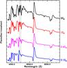 |
Fig. 1 Model spectra (D14) from four distinct progenitor models at 50 days post explosion: 0.1, 0.4, 1 and 2 × solar metallicity. The dotted black lines bracket the Fe ii 5018 Å absorption feature we use in this analysis. |
Data reduction was performed in the standard manner using iraf, in the form of: bias-subtractions; flat-field normalisations; 1d spectral extraction and sky-subtraction of emission line spectra; and finally wavelength and flux calibration. One dimensional spectral extraction was first achieved on the exact region where each SN exploded. However, in many cases no emission lines were detected in that region (consistent with the non-detection of Hα within SN II environments as reported in Anderson et al. 2012), and extractions were attempted further along the slit in either direction until sufficient lines (at a minimum Hα and [N ii]) could be detected. The distances of these extraction regions from those of SN explosion coordinates are listed in Table B.1, and the effect of including H ii-region measurements offset from explosion sites is discussed below.
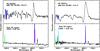 |
Fig. 2 Two examples of both SN II spectra (upper panels, at epochs close to 50 days post explosion) and host H ii-region spectra (lower panels). Left: SN 2003bl, a SN with relatively high Fe ii 5018 Å pEW and O3N2 abundance, and right: SN 2007oc with relatively low Fe ii 5018 Å pEW and O3N2 abundance. The position of the Fe ii 5018 Å absorption feature in the SN spectra is indicated in blue. In the H ii-region spectra we indicate the position of the emission lines used for abundance estimations: Hβ in green, [O iii] in cyan, Hα in blue, and [N ii] in magenta. |
2.3. Synthetic spectra of SN IIP at different metallicities
The observational research presented in this manuscript was motivated by the study of D14. That study used four models with distinct progenitor metallicities, producing synthetic spectral time series. Progenitors of 15 M⊙ initial mass, and progenitor metallicities of 0.1, 0.4, 1, and 2 times solar (Z⊙) were evolved from the main sequence until death with mesa (Paxton et al. 2011) – adopting Z⊙ = 0.02. Upon reaching core-collapse, progenitors were exploded and synthetic spectral sequences computed using cmfgen (Dessart & Hillier 2010; Hillier & Dessart 2012). The reader is referred to Dessart et al. (2013) and D14 for a detailed explanation of the modelling procedure (Dessart et al. 2013 explore a large range of progenitor parameters and their subsequent effects on the model SNe II produced, while D14 concentrates on the effect of progenitor metallicity).
In Fig. 1 model spectra are plotted, one for each progenitor metallicity, taken at 50 days post explosion (50 d). One can clearly see the effects of increasing metallicity on the model spectra, in particular at bluer wavelengths (i.e. bluewards of Hα,  6000 Å). The higher metallicity models exhibit many more lines which are also significantly stronger in EW. As one goes to the lower metallicity models spectra appear much “cleaner” being dominated by Balmer lines and showing weaker signs of metal line blanketing.
D14 explored the effects of changing progenitor metallicity with all other parameters constant (initial mass, mass-loss and mixing length prescriptions). However, there are other pre-SN parameters which may significantly affect the evolution and strength of spectral line EWs (the important features we use in the current work), and produce degeneracies in SN measurements. D14 showed how SNe II with distinct pre-SN radii (created using the same progenitors, but evolved with a distinct mixing length prescription for convection) produced different EW strengths and evolutions for the same progenitor metallicity. This is seen in Figs. 4 and 10, where the models are referred to as m15mlt1 (larger radius) and m15mlt3 (smaller radius, m15mlt2 is the solar metallicity model already discussed above). We use such models to compare the metal line EWs resulting from metal abundance variations or from changes in the progenitor structure.
3. Analysis
As outlined above, our data comprises two distinct sets, and hence our analysis is split into two distinct types of measurements. These are now outlined in more detail. In Fig. 2 we present examples of our data, indicating the position of the spectral lines used in our analysis.
3.1. SNe II Fe II 5018 Å EW measurements
To quantify the influence of progenitor metallicity on observed line strengths, in this publication we concentrate on the strength of the Fe ii 5018 Å line. This line is prominent in the majority of SNe II from relatively early times, i.e. at the onset of hydrogen recombination, and stays present throughout the photospheric phase. In addition, it is not significantly contaminated by other SN lines. One issue with this line is that it is in the wavelength range where one observes narrow Hβ and [O iii] emission lines from host H ii regions. Often it is difficult to fully remove these features in spectral reduction and extraction, and they can contaminate the broad spectral features of the SN. When narrow H ii-region emission lines are present in our SN spectra, they are removed by simply interpolating the SN spectra between either side of the emission line. The uncertainty created by this process is taken into account when estimating flux errors. pEWs are measured in all spectra obtained within 0−100 days post explosion (see A14 for details of explosion epoch estimations). To measure pEWs we proceed to define the pseudo continuum (the adjacent maxima that bound the absorption) either side of the broad SN absorption feature and fit a Gaussian. These are defined as “pseudo” EWs due to the difficulty in knowing/defining the true continuum level. This procedure is achieved multiple times, each time removing narrow emission lines when present. A mean pEW is then calculated together with a standard deviation, with the latter being taken as the pEW error. In this way we obtain a pEW for each spectral epoch. The same measurement procedure undertaken for observations is achieved for model spectra, meaning that for models we also present pEWs to make consistent comparisons with observations (even though in the case of models we know the true continuum and could measure true EWs).
3.2. Host H II-region abundance measurements
Fluxes of all detected narrow emission lines within host H ii-region spectra are measured by defining the continuum on either side of the emission and fitting a Gaussian to the line. The lines of interest for our abundance estimations are: Hβ, [O iii], Hα, and [N ii]. Using these fluxes, gas-phase oxygen abundances are calculated using the N2 and O3N2 diagnostics of both M13 and the earlier calibrations from Pettini & Pagel (2004). These are listed in Table B.1. Abundance errors are estimated by calculating the minimum and maximum line ratios taking into account line flux errors, i.e. the “analytic” approach outlined in Bianco et al. (2015; and used on the previous sample of Anderson et al. 2010). In addition, in Figs. 8 and 9 the systematic errors from the M13 N2 and O3N2 diagnostics are also shown.
We are restricted in the abundance diagnostics we can use simply because of small number of detected emission lines in our data. Our exposure times were relatively short so in many cases only Hα and [N ii] are detected, making the N2 diagnostic the only possibility. An advantage of both the N2 and O3N2 diagnostics is that they are essentially unaffected by either host-galaxy extinction and/or relative flux calibration, due to the use of ratios of emission lines close in wavelength. While both the M13 and Pettini & Pagel (2004) abundances are listed in Table B.1, we use the M13 values for our analysis given the recalibration of the diagnostics including additional H ii-region Te measurements3.
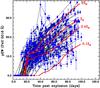 |
Fig. 3 Evolution of Fe ii 5018 Å pEWs with time for all SNe II within the sample. Individual measurements are shown in blue, together with their errors. These are connected by black lines. Also presented are the time sequence of pEWs measured from synthetic spectra (Dessart et al. 2013), for four models of distinct progenitor metallicity. |
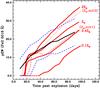 |
Fig. 4 Same as Fig. 3, but now the observational data are binned in time. The black sold line represents the mean pEW within each time bin, while the dashed blue lines indicate the standard deviation. Together with the four distinct metallicity models (Dessart et al. 2013 shown in solid red lines) we also present spectral series produced from two additional solar metallicity progenitors, but with distinct mixing length prescriptions, leading to smaller (mlt3, shown as the dotted red line) and larger (mlt1, shown as the dashed red line) RSG progenitor radii (see Sect. 2.3 for more details). |
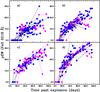 |
Fig. 5 Evolution of Fe ii 5018 Å pEWs with time, as presented in Fig. 3, separated into 4 panels splitting the sample by their Fe ii 5018 Å pEWs at 50 d. The distributions go from low pEW in panel a) through to the highest pEW sample in panel d). The overall sample is presented in blue, while the “Gold” sample discussed later is plotted in magenta. (Errors are not plotted to enable better visualisation of the trends.) |
4. Results
Above we have presented two sets of observations: spectral line Fe ii 5018 Å pEW measurements during the photospheric phase of SNe II, and emission line spectral measurements of SN II host H ii regions, with the latter being used to obtain environment oxygen abundances. The distributions of these are now both presented. Then we proceed to correlate both parameters, and confront model predictions with SN and host H ii-region observations. In addition, we analyse how pEWs are related to other SN II light-curve and spectral parameters, and finally we search for correlations between environment metallicity and SN II transient properties.
4.1. Fe II 5018 Å pEW distribution and evolution
The time evolution of SN pEWs is shown in Fig. 3, together with those from spectral models. In Fig. 4 we present these same measurements but now with the observations binned (with bins of 0−20 days, then 20−30, 30−40, 40−50, 50−60, 60−70, 70−80, and 80−100 days). In both figures the evolution of model pEWs is also presented. These figures show the increase in time of pEWs (using the convention that a deeper absorption is documented as a larger positive pEW), but also the large dispersion between different SNe II. One can also see the distinct strength and evolution of Fe ii 5018 Å pEWs found within model spectra from the four distinct progenitor metallicities. The effect on model spectra of changing pre-SN radii (at a fixed, solar, metallicity) can be seen in Fig. 4 (m15mlt1 larger radius, and m15mlt3 smaller radius).
In Fig. 5 the pEW – time past explosion trends from Fig. 3 are again presented but now split into 4 panels, separating SNe by their pEWs at 50 d post explosion (see below for discussion of this measurement). It is now possible to observe the trends of individual SNe in more detail. This confirms the monotonic behaviour of Fe ii 5018 Å pEWs with time past explosion throughout the “plateau” phase of SNe II evolution (<100 days post explosion), in qualitative agreement with models. The plot also shows that SNe with similar pEWs at 50 d evolve in a similar manner with relatively low dispersion.
To proceed with our analysis pEWs are required at consistent epochs between SNe. Our epoch of choice is 50 d (more details below). To estimate the pEW at this epoch, interpolation/extrapolation is needed. This is achieved for SNe II with ≥2 measurements available and where in the case of extrapolation, a spectrum is available at 50 ± 10 days post explosion. Then a low order polynomial fit is made to the pEW measurements, and this is used to obtain a pEW at 50 d. We use the rms error of this fit as the error on the interpolated pEW. This interpolation was possible in 82 cases, and a histogram of these measurements is presented in Fig. 6.
4.2. Host H II-region abundances
In Fig. 7 we present the distribution of all SN II emission line abundance measurements for both the N2 and O3N2 M13 diagnostics. The N2 distribution has a mean value of 12+log[O/H] = 8.49 dex, and a median of 8.52 dex. The distribution shows a peak at just below ~8.6 dex, and a tail out to lower abundances with the lowest value of 8.03 dex. The O3N2 distribution has a mean of 8.41 dex, and a median value of 8.44 dex. The distribution shows a peak at ~8.5 dex, a range of ~0.6 dex, and a tail out to lower abundances with the lowest value of 8.06 dex. Using a solar value of 12+log[O/H] = 8.69 dex (Asplund et al. 2009), the O3N2 distribution thus ranges between 0.23 and 0.87 Z⊙, with a mean of 0.51 Z⊙. However, we stress that any discussion of absolute metallicity scale when dealing with emission line diagnostics is problematic, and it is probable that the N2 and O3N2 diagnostics give systematically lower abundances than the true intrinsic values (see e.g. López-Sánchez et al. 2012, and references therein).
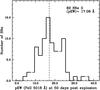 |
Fig. 6 Histogram of Fe ii 5018 Å pEW measurements for our sample of SN II spectra, interpolated to 50 d. The position of the mean pEW is indicated by the vertical dashed line. |
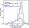 |
Fig. 7 M13 N2 and O3N2 abundance distributions, together with their mean values (dashed lines). |
4.3. SN II Fe II 5018 Å pEWs and host H II region abundance
In Fig. 8 SN II Fe ii 5018 Å pEWs at 50 d are plotted against the N2 diagnostic on the M13 scale. To test the significance of this trend, and all subsequent correlations, we run a Monte Carlo simulation randomly selecting events from the distribution in a bootstrap with replacements manner 10 000 times. The mean Pearson’s correlation r value is determined together with its standard deviation using the 10 000 random sets of pEW – abundances. The lower limit of the chance probability of finding a correlation, p, is then inferred using these values4. With a total of 82 events which have SN II Fe ii 5018 Å pEWs and N2 oxygen abundance measurements, we find r = 0.34 ± 0.09, and a chance probability of finding a correlation of ≤2.4%. Statistics using only the observed distribution give: r = 0.34, p = 0.18%. Hence, using N2 we find a moderate strength correlation between SN pEW and host H ii-region abundance. It is clearly observed that there is a lack of SNe II with high pEW and low abundance at the bottom right of Fig. 8. There are fewer SN environments where we were able to also measure (in addition to Hα and [N ii]) the Hβ and [O iii] fluxes needed to compute abundances on the O3N2 scale. We are able to do this in 44 cases, and here we obtain a mean r value of 0.50 ± 0.10, which gives a chance probability of ≤0.7%. Statistics using only the observed distribution give: r = 0.50, p = 0.05%. The correlation is shown in Fig. 9. While the statistical significance is higher for the O3N2 diagnostic (and therefore we use that diagnostic for subsequent sub-samples), both of these figures show there is a statistically significant trend in the direction predicted by models: SNe II with larger Fe ii 5018 Å pEWs tend to be found in environments of higher oxygen abundance. These observational results hence agree with model predictions, and motivate further work to use SNe II as environment metallicity indicators. We also note that the rms errors on the M13 N2 and O3N2 diagnostics (as plotted in Figs. 8 and 9), appear to be large when compared to the spread of values in our plots. Given that we do find evidence for correlation, this suggests the true precision of those diagnostics for predicting H ii-region abundance is better than the values given by M13.
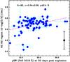 |
Fig. 8 pEW of the Fe ii 5018 Å absorption line measured at 50 d plotted against host H ii-region oxygen abundance on the N2 M13 scale. The dashed line indicates the mean best fit to the data. Error bars on individual measurements are the statistical errors from line flux measurements. The large black error bar gives the N2 diagnostic error from M13. |
In Fig. 10 we over-plot SN II models at four different metallicities, together with the additional two models at solar metallicity but with different pre-SN radii (D14), onto the observed Fe ii 5018 Å pEW vs. H ii-region abundance plot. The model metallicities are converted from fractional solar to oxygen abundance using a solar value of 8.69 dex (Asplund et al. 2009). One can see that the models produce a much steeper trend than that observed. We also see that models with the same progenitor metallicity but with different pre-SN radii produce a range of almost 10 Å in Fe ii 5018 Å pEWs. This uncertainty can be reduced with a slight time shift (of pEW measurements) or by comparing at a given colour (see below for additional analysis). However, in general, SN II observations favour relatively low progenitor radii (Dessart et al. 2013; González-Gaitán et al. 2015), and explosions similar to that of the large radius model are probably rare in nature. Therefore the actual uncertainty in observed SNe II is probably less than that represented by this range of models. Another interesting observation from Fig. 10 is the lack of any SN close to the tenth solar model. There is also a lack of SNe II at super-solar values. We discuss this (possibly small) range of metallicities probed by observations below.
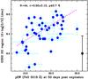 |
Fig. 9 Same as Fig. 8, but now for the O3N2 diagnostic on the M13 scale. The dashed line indicates the mean best fit to the data. Error bars on individual measurements are the statistical errors from line flux measurements. The large black error bar gives the O3N2 diagnostic error from M13. |
4.3.1. Sub-samples
In Figs. 8 and 9 all SNe II were included irrespective of their light-curve or spectral properties. This means that we include SNe II with a wide range of absolute magnitudes, “plateau” decline rates (s2), and optically thick phase durations (OPTd) (and other SN parameters which differ from one event to the next). The models of D14 all produce SN light-curves and spectra typical of “normal” SNe IIP. In addition, those figures included all SN II abundance measurements, including events with abundances estimated from a region of their host galaxies at significant distances from explosion sites. Here these issues are further investigated.
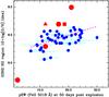 |
Fig. 10 Comparison of the D14 models with observations. pEWs of the Fe ii 5018 Å absorption line measured at 50 d plotted against the host H ii-region oxygen abundance using the O3N2 M13 diagnostic, with the positions of the six distinct models over plotted. The red circles indicate the same progenitors changing metallicity, while the triangle (m15mlt1, larger radius) and square (m15mlt3, smaller radius) present the same metallicity but changing pre-SN radii. |
Epoch of pEW measurements: testing the level of correlation between Fe ii 5018 Å pEWs and host H ii-region abundances when different epochs for pEW measurements are used.
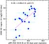 |
Fig. 11 “Gold IIP” sample of pEWs against O3N2 abundances, using SNe II with s2 values ≤1.5 mag per 100 days, and/or OPTd values ≥70 days. |
First we construct a sub-sample of events where abundance estimations were carried out less than 2 kpc away from the explosion sites5. When this is achieved we are left with 56 SNe II with measurements on the N2 scale and 32 on the O3N2 scale. We again test for correlation using Monte Carlo bootstrapping with replacements, and in the case of N2 a correlation coefficient r of 0.42 ± 0.10 is found, giving a chance probability (N = 56) of ≤1.6%. Using O3N2 we obtain r = 0.55 ± 0.10 and a p value of ≤1.0% (N = 32). The level of correlation thus increases when we only include abundance measurements closer to SN explosion sites. This is to be expected, as SNe II have relatively short lifetimes and are therefore not expected to move significantly from their birth sites. As one moves away from exact explosion sites environment metallicity becomes less representative of progenitor abundance due to spatial metallicity changes from one region of a galaxy to another, especially in terms of increasing/decreasing galacto-centric offset.
To produce a sub-sample of “normal” SNe IIP cuts are made to our sample in terms of light-curve morphologies. SNe II with s2 values ≥1.5 mag per 100 days, and/or OPTd values ≤70 days are removed from the sample. Using these cuts a “Gold IIP” sample of 22 SNe II is formed, which would generally be considered typical SNe IIP by the community. Testing for correlation, this sub-sample has an r value = 0.68 ± 0.10 and a p value = ≤0.5%. This correlation is presented in Fig. 11, and shows the increase in strength of correlation as compared to the full O3N2 sample in Fig. 9 (characterised by r = 0.50 ± 0.10). The fast declining (s2 ≥ 1.5 mag per 100 days) sample presents a lower level of correlation (than that of the ‘normal’ SNe IIP): for 15 SNe, r = 0.57 ± 0.18 and p = ≤ 4.6%. Both the “Gold IIP” and fast-declining samples show the same linear trends within their errors. This suggests that “normal” SNe IIP are better metallicity indicators than their faster declining counterparts.
4.3.2. The epoch of pEW measurements
Above we presented the pEW distribution and then correlations with H ii-region abundances using Fe ii 5018 Å pEWs at 50 d. This epoch was chosen as it corresponds to when the vast majority of SNe II are around halfway through the photospheric phase of their evolution. SNe II can show significant temperature variations at early times and one does not want to measure pEWs when temperature differences could be a significant factor controlling their strength. Fig. 4 also shows that pEWs have a rapid increase at early times after first appearing at ~15 days, and therefore one wants to avoid this region where non-metallicity systematics may dominate differences in pEWs. At much later than 50 d some SNe II already start to transition from the photospheric phase to radioactively powered epochs. Here, pEWs may start to be affected by mixing of He-core material (in addition to the fact that spectral observations become more sparse). We now test whether this selected epoch is the most appropriate to measure pEWs.
pEW measurements are interpolated to: 30, 40, 60 and 70 days post explosion. These values are then correlated against host H ii-region abundances on the N2 scale (used to ensure sufficient statistics for valid comparisons) and the strength of the correlations are compared. In addition, in place of the explosion epoch, pEWs are estimated with respect to ttran: the epoch of transition from the initial s1 decline to the slower “plateau” s2 phase (see A14 for details of those measurements). We choose the epoch ttran+20 days, which roughly coincides with 50 d, but varies (approximately ±10–15 days) between SNe II. The results of these comparisons are presented in Table 1. In terms of time post explosion we see that the choice of 50 days is in fact valid. Its is also observed that 50 d does just as well as ttran+20 days. A time epoch with respect to OPTd is also investigated (OPTd is the OPtically Thick phase time duration, from explosion to the end of the “plateau”, A14). pEWs are interpolated to OPTd−30 days (again to coincide on average with t = ~ 50 d), and we run our correlation tests for both this new OPTd sample, and the same SNe II but with pEWs at 50 d. Values are again displayed in Table 1, and it is found that using OPTd as the time epoch is no better than using the explosion epoch. In conclusion the choice of 50 d for pEW measurements appears to be robust.
Now, in place of time, we investigate whether a stronger correlation exists if pEWs are measured at a colour epoch. As already seen in the D14 spectral models: differences in pre-SN properties can significantly affect the strength of spectral lines (see Figs. 4, 10). Together with the metal abundance within the ejecta, the other main contributor to line appearance and subsequent strength is the temperature/ionisation of the line formation region. Models corresponding to different progenitor radii produce SNe II with distinct temperature evolution. Therefore, examining observational pEWs at a consistent colour (i.e. temperature) may be of interest.
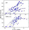 |
Fig. 12 Evolution of Fe ii 5018 Å pEWs with SN colour. In the top panel the CSP sample is shown using the V−i colour, while in the bottom panel the CATS et al. sample using V−I is presented. (Errors on colours and pEWs are not presented to enable better visualisation of trends.) |
Figure 12 presents the evolution of pEWs with SN colour (using the sample defined below). This confirms the behaviour discussed above: pEWs increase with increasing SN colour.
A major issue with any colour analysis is correction for extinction in the line-of-sight within host galaxies. However, as discussed in detail in Faran et al. (2014b), without detailed modelling and early-time data (see e.g. Dessart et al. 2008), there is no current satisfactory method for accurately correcting SNe II for host galaxy reddening. This is particularly pertinent for the current study where our goal is to obtain differences in intrinsic colours (i.e. assuming SNe II have similar colours during the plateau would simply lead us to use a time epoch). Another complication is that the CSP and previous CATS et al. samples do not have the same filter observations.
To continue the investigation we proceed in the following manner. To begin, all SNe II having host galaxy AV values published in A14 higher than 0.1 mag, or where no AV estimate was possible because either the pEW of narrow ISM sodium lines was higher than 1 Å, or where the upper limit of this quantity was higher than 1 Å, are removed from the sample. We then assume that the rest of the sample is effectively free of significant host galaxy reddening. For all SNe II within the CSP sample we create V−i colour curves, while for the CATS et al. samples V−I colour curves (both corrected for MW extinction) are produced6. Low-order polynomials are fit to these colour curves and we then interpolate to measure the colour at 50 d. For each sample (CSP/CATS et al.) a mean 50 day V−i/V−I colour is calculated. For each individual SN we proceed to measure a pEW for Fe ii 5018 Å at the corresponding mean colour epoch. This method negates any need to convert i-band magnitudes into I, or vice versa, and is valid if it is assumed that the CSP and CATS et al. samples are drawn from the same underlying SN II distribution.
In Fig. 13 we plot Fe ii 5018 Å pEWs at these colour epochs against host H ii-region abundance on the O3N2 scale. Testing for correlation we find, for N = 17, r = 0.69 ± 0.12 and p ≤ 1.7%, while for the same SNe II but with pEWs measured at 50 d we find r = 0.61 ± 0.16 and p ≤ 7.0%. This suggests that in using a colour epoch in place of time, one further removes SN systematics and strengthens the case for SNe II to be used as metallicity indicators.
Statistics of correlations between Fe ii 5018 Å pEWs and SN II light-curve and spectral parameters. In the first column the SN II parameter is listed.
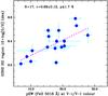 |
Fig. 13 SN II pEWs against O3N2 abundances for the V−i/V−I colour sample. |
4.4. Correlations between pEWs and other SN II parameters
Here we correlate pEWs at 50 d with the SN II light-curve and spectral parameters presented by A14 and Gutiérrez et al. (2014). The statistical significance of correlations between pEWs and these parameters are listed in Table 2. A full discussion of these correlations, together with figures and discussion of their implications for our understanding of SNe II explosions and progenitors will be left for a future publication (Gutíerrez et al. in prep.). However, there are some interesting trends seen in Table 2 and we briefly discuss those now.
The absolute magnitude at maximum light, Mmax, of SN II is found to strongly correlate with the Fe ii 5018 Å pEW at 50 d. Indeed, while the pEW also shows correlation with Mend and Mtail (all in the sense that brighter SNe II have lower pEWs at a consistent time epoch), the strength of the correlation is less. This is in agreement with A14, where Mmax was shown to be a more important parameter in understanding the diversity of SNe II than the end of “plateau” magnitude Mend. The decline rates, s1, s2 and s3, all show some degree of correlation with the Fe ii 5018 Å pEW in the direction that slower decliners have higher pEWs. Interestingly, when we include upper limits, 56Ni masses show a strong correlation with pEWs: SNe II which produce more nickel have lower pEWs. The time duration OPTd, i.e. the time between explosion and the end of the “plateau” together with Pd (ttran to end of “plateau”) show zero correlation with pEWs. Finally, the spectral parameters a/e (the ratio of the pEW of absorption to emission of Hα) and the FWHM velocity of Hα (see Gutiérrez et al. 2014 for more details) both show a strong correlation with pEWs. SNe II with large pEWs at 50 d have larger a/e values and smaller velocities.
4.5. The influence of metallicity on SN II diversity
We test for correlation between SN II host H ii-region abundance and light-curve and spectral parameters. No evidence for correlation is found between abundance and any SN II parameter, except that with metal line pEWs. In Figs. 14−16 we show host H ii-region abundance plotted against Mmax, s2, and OPTd respectively. One can see that no trends appear. In Table 3 the results of statistical tests for trends between these parameters and host H ii-region abundance, together with all other SN II light-curve and spectral properties presented in A14 and Gutiérrez et al. (2014) are shown. In addition, we repeat the statistics for the correlation between SN II Fe ii 5018 Å pEWs and host H ii region abundance already presented above. It is clear that the only (thus far measured/presented) SN II parameter which shows any correlation with environment metallicity is the Fe ii 5018 Å pEW.
These results suggest that the diversity of SN II properties in the current sample does not stem from variations in metallicity – either the range in metallicity is too small to matter (which is likely) or some other stellar parameter (e.g. main sequence mass) is more influential.
Statistics of correlation tests between host H ii-region abundance, and SN II light-curve and spectral parameters.
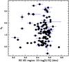 |
Fig. 14 Host H ii-region oxygen abundance plotted against SN II “plateau” decline, s2. |
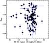 |
Fig. 15 Host H ii-region oxygen abundance plotted against SN absolute V-band maximum, Mmax. |
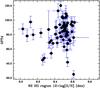 |
Fig. 16 Host H ii-region oxygen abundance plotted against SN OPTd: time duration from explosion to end of “plateau”. |
5. Discussion
Dessart et al. (2014) presented SN II model spectra produced by progenitors of distinct metallicity, and showed how the strength of metal lines increases with increasing progenitor metallicity. Those models therefore made a prediction that SNe II with higher metal line pEWs will be found in environments of higher metallicity. In this publication we have concentrated on the strength of the Fe ii 5018 Å line as measured in observed SN II spectra, and shown that indeed the pEW of this line shows a statistically significant trend with host H ii-region abundance, with the latter derived from the ratio of H ii-region emission lines. We now discuss this result in more detail, and outline the next steps to use SNe II as independent environment metallicity probes. The implications of the above results on the progenitors and pre-SN evolution of SNe II are also further explored.
5.1. The use of photospheric phase SN II spectra as independent metallicity indicators
The aim of this work is to confront model predictions with observations to probe the accuracy of SNe II as metallicity indicators. The correlation observed between SN Fe ii 5018 Å pEW and host H ii-region abundance suggests that SNe II may be at least as accurate at indicating environment metallicity as the popularly used N2 and O3N2 diagnostics. This is inferred from Figs. 8, 9, 11, and 13. The dispersion within these correlations is similar to (or better than) the internal dispersion of the emission line diagnostics. This probably implies that a) the majority of the dispersion on the pEW-abundance plots arises from the diagnostics and not the SN measurements; and b) the rms values of M13 underestimate the true precision of N2 and O3N2. This finding motivates work to use SNe II as metallicity indicators independent of these emission line diagnostics.
Currently there is a lack of SNe II within this sample at both low (sub-LMC) and high (super-solar) metallicities (although we caution that the latter may be due to the saturation of the M13 diagnostics at above ~solar metallicity). Finding SNe II within these environments and adding these to the sample would allow metallicity differences to dominate changes in pEW, and lend further support to the use of SN II as metallicity probes. A first step to remove the calibration from strong emission line diagnostics could be to obtain deeper spectra of the host H ii regions to enable detections of emission lines which provide electron temperature estimates, i.e. the direct method. In this case SNe II would still be tied to the same scale as those diagnostics used throughout the Universe. One may look at models to calibrate the SN observations. However, to do this accurately would probably require individual fitting of each SN to a large grid of spectral models. Currently, what we can state with confidence is that an observed SN II at ~50 d days post explosion with a pEW< 10 Å suggests an environment metallicity of less than or equal to LMC metallicities (0.2 Z⊙). At the other extreme, if one finds a SN II with an Fe ii 5018 Å pEW~> 30 Å, this implies the SN exploded within a ~solar abundance (12+log[O/H] = 8.69 dex, Asplund et al. 2009) region or higher.
5.2. Progenitor metallicity as a minor player in producing SN II light-curve and spectral diversity?
Metallicity is thought to be a key ingredient in stellar evolution, driving the extent of mass-loss through metallicity dependent stellar winds. However, a major finding presented here is of zero evidence for correlation between SN parameters and environment abundance (except in the case of the pEW of metal lines affected by the nascent composition of the SN ejecta). This suggests metallicity is in fact playing a negligible role in producing the diversity observed in the current sample. However, we suspect the range in metallicity is too narrow to drive SN II diversity. There are many other parameters which likely change within our sample such as progenitor mass, mass-loss rates, degree of binary interaction etc. It may be that when we eventually probe a larger range of metallicity we start to see the effects of progenitor metallicity on SN diversity. It is noted however that even if our sample lacks SNe II in the extremes of the metallicity distribution, the rate of these events is unlikely to be significant compared to the current sample. In conclusion, over the range of progenitor metallicities we have in our current sample, chemical abundance is not a driving force in producing SN II light-curve and spectral diversity.
5.3. The lack of SNe II in low-metallicity environments
The lack of SNe II in low metallicity environments (e.g. those found in the Small Magellanic Cloud or lower) was already noted in Stoll et al. (2013) and D14. In the current analysis we now have additional constraints through our environment abundances. In a sample of 115 (52) SNe II on the N2 (O3N2) scale, the lowest metallicity environment is that of SN 2003cx, at an oxygen abundance of 8.03 (8.06) dex on the N2 (O3N2) scale. Using the solar abundance of 8.69 dex (Asplund et al. 2009) this translates to 0.22 Z⊙, i.e. ~abundances found in the LMC. As noted above and discussed in López-Sánchez et al. (2012), the N2 and O3N2 scales give systematically lower abundances than those from other emission line methods. If this is the case then the lack of low-metallicity environment SNe II would become even more apparent. There also appears to be a lack of SNe II in super-solar metallicity environments. However, if we accept that the N2 and O3N2 scales give systematically low abundances, then this may become less significant.
Other SN II environment metallicities have been published. For sake of comparison we calculate our distributions now on the Pettini & Pagel (2004) scale (see Table B.1). On this scale a mean N2 abundance =8.62 ± 0.21 dex and a mean O3N2 abundance = 8.55 ± 0.21 dex is found. Anderson et al. (2010) published a sample of 46 SNe II oxygen abundances and derived a very similar distribution as that found here, which is unsurprising given that about half of those values are included in our sample. Kuncarayakti et al. (2013) analysed very nearby SNe II environments and found a mean 12+log[O/H] value of 8.58 dex for 15 SNe II, again very similar to our sample. One common parameter between these samples is that the SNe II were generally found via galaxy targeted searches, and therefore they may be biased towards more massive, higher metallicity galaxies. Indeed, the Palomar Transient Factory (PTF, Rau et al. 2009) published a distribution of CC SN host galaxy absolute magnitudes which probed a greater number of dwarf galaxies than found in, e.g. our sample (see further discussion in the appendix of A14). However, Stoll et al. (2013) obtained emission line spectra of the host H ii regions of a representative sample of PTF SN II hosts, and concluded that the abundance distribution was indistinguishable from that found in targeted samples (e.g. Anderson et al. 2010). In conclusion, there appears to be a true lack of (published) SNe II found with SMC or lower metallicities. Finding and studying such SNe II will not only serve our analysis to further calibrate SNe II as metallicity probes, but will also allow the study of how massive stars explode at low metallicity.
5.4. Future directions
In this work we have focussed on the dependence of the pEW of a single spectral line Fe ii 5018 Å on environment metallicity. In future work we will analyse the full distribution of SN photospheric phase metal line strengths to determine the most direct indicator of progenitor metallicity. In addition, we are currently limited to a relatively small range in metallicity. Observing additional SNe II outside of this range will aid in removing other systematic uncertainties in the correlations we have presented.
While there is still much to understand, the ultimate aim of this work would be to independently map the metallicity distribution of galaxies throughout the Universe using SNe II. To aid in this goal one may think of observing SNe II in both a range of environments and out to higher redshifts. The advantage of SNe II over traditional metallicity indicators is that a) they probe the specific location where they explode within their hosts; b) in principle one can obtain abundances of distinct elements and not simply oxygen; and c) SNe II are intrinsically bright thus the currently proposed metallicity diagnostic can be efficient – in terms of telescope observing time – for probing distant galaxies. In terms of constraining a range of relative metal abundances it is important to calibrate all metal lines within SNe II spectra, and understand the systematics in their measurements and metallicity predictions. SNe II explosions accurately trace the star formation within galaxies (e.g. Botticella et al. 2012). Hence, mapping metallicity with SNe II discovered by un-targeted searches will accurately trace the chemical abundance of star-forming regions within galaxies.
6. Conclusions
Following the study of D14, we present observations of a large sample of SN II host H ii-region spectroscopy from which gas-phase oxygen abundances are inferred. These are compared to pEW measurements of Fe ii 5018 Å and a statistically significant trend is observed, in that SNe II with higher pEWs explode in higher metallicity environments. This paves the way for the use of SNe II as independent metallicity indicators throughout the Universe. While we observe significant dispersion in this trend, this is expected because a) the SNe II included show many different properties; and b) the abundance diagnostic used for comparison itself shows significant dispersion in its correlation with electron temperature. Indeed, the significance of correlation is increased if we only consider: a) H ii-region measurements close to explosion sites; b) SNe II which have light-curve morphologies similar to “normal” SNe IIP; and c) if we use a colour epoch for pEW measurements in place of time.
We also search for trends of progenitor (inferred from environment) metallicity with various SN II light-curve and spectral parameters. However, no such trends are observed. We therefore conclude, that at least within the current sample, progenitor metallicity plays a negligible role in producing the observed diversity of SNe II.
HyperLeda: http://leda.univ-lyon1.fr/
iraf is distributed by the National Optical Astronomy Observatory, which is operated by the Association of Universities for Research in Astronomy (AURA) under cooperative agreement with the National Science Foundation.
If we were to use the Pettini & Pagel (2004) values instead then our results and conclusions remain unchanged.
It is generally considered that for r values between 0.0 and 0.2 there is zero or negligible correlation; between 0.2 and 0.3 weak correlation; between 0.3 and 0.5 moderate correlation; and above 0.5 signifies strong correlation. The p value gives the probability that this level of correlation is found by chance.
This limit is somewhat arbitrary, however it removes cases where extractions are at a significant distance from explosion sites, while maintaining a sufficient number of events to enable a statistically significant analysis.
Note, CATS et al. photometry was published in Galbany et al. (2016), while CSP optical photometry will be published in Anderson et al. (in prep.), and a full colour analysis of the latter concentrating on host galaxy extinction will be provided in de Jaeger et al. (in prep.).
Acknowledgments
The annonymous referee is thanked for their useful comments which helped clarify some important points in the paper. Support for C.G., M.H., L.G. and H.K. is provided by the Ministry of Economy, Development, and Tourism’s Millennium Science Initiative through grant IC120009, awarded to The Millennium Institute of Astrophysics, MAS. L.G. and H.K. acknowledge support by CONICYT through FONDECYT grants 3140566 and 3140563 respectively. L.D. acknowledges financial support from “Agence Nationale de la Recherche” grant ANR-2011-Blanc-BS56-0007. The work of the CSP has been supported by the National Science Foundation under grants AST0306969, AST0607438, and AST1008343. M. Stritzinger gratefully acknowledges the generous support provided by the Danish Agency for Science and Technology and Innovation realized through a Sapere Aude Level 2 grant. Based on observations made with ESO telescopes at the La Silla Paranal Observatory under pro- gramme: 094.D-0283(A). A special thanks goes to the ANTU support staff at Paranal observatory for obtaining the observations used in this publication. In particular we acknowledge the telescope and instrument operators: Israel Blanchard, Claudia Cid, Alex Correa, Lorena Faundez, Patricia Guajardo, Diego Parraguez, Andres Parraguez, Marcelo Lopez, Julio Navarrete, Leonel Rivas, Rodrigo Romero, and Sergio Vera. This research has made use of the NASA/IPAC Extragalactic Database (NED) which is operated by the Jet Propulsion Laboratory, California Institute of Technology, under contract with the National Aeronautics.
References
- Anderson, J. P., Covarrubias, R. A., James, P. A., Hamuy, M., & Habergham, S. M. 2010, MNRAS, 407, 2660 [NASA ADS] [CrossRef] [Google Scholar]
- Anderson, J. P., Habergham, S. M., James, P. A., & Hamuy, M. 2012, MNRAS, 424, 1372 [NASA ADS] [CrossRef] [Google Scholar]
- Anderson, J. P., Dessart, L., Gutierrez, C. P., et al. 2014a, MNRAS, 441, 671 [NASA ADS] [CrossRef] [Google Scholar]
- Anderson, J. P., Gonzàlez-Gaitàn, S., Hamuy, M., et al. 2014b, ApJ, 786, 67 [NASA ADS] [CrossRef] [Google Scholar]
- Appenzeller, I., Fricke, K., Fürtig, W., et al. 1998, The Messenger, 94, 1 [NASA ADS] [Google Scholar]
- Arcavi, I., Gal-Yam, A., Cenko, S. B., et al. 2012, ApJ, 756, L30 [NASA ADS] [CrossRef] [Google Scholar]
- Asplund, M., Grevesse, N., Sauval, A. J., & Scott, P. 2009, ARA&A, 47, 481 [NASA ADS] [CrossRef] [Google Scholar]
- Barbon, R., Ciatti, F., & Rosino, L. 1979, A&A, 72, 287 [Google Scholar]
- Bianco, F. B., Modjaz, M., Oh, S. M., et al. 2015, Astrophysics Source Code Library, [record ascl:1505.025] [Google Scholar]
- Blinnikov, S. I., & Bartunov, O. S. 1993, A&A, 273, 106 [NASA ADS] [Google Scholar]
- Botticella, M. T., Smartt, S. J., Kennicutt, R. C., et al. 2012, A&A, 537, A132 [NASA ADS] [CrossRef] [EDP Sciences] [Google Scholar]
- Contreras, C., Hamuy, M., Phillips, M. M., Folatelli, G., et al. 2010, AJ, 139, 519 [NASA ADS] [CrossRef] [Google Scholar]
- Covarrubias, R. A. 2007, Ph.D. Thesis, University of Washington [Google Scholar]
- Dessart, L., & Hillier, D. J. 2010, MNRAS, 405, 2141 [NASA ADS] [Google Scholar]
- Dessart, L., Blondin, S., Brown, P. J., et al. 2008, ApJ, 675, 644 [NASA ADS] [CrossRef] [Google Scholar]
- Dessart, L., Hillier, D. J., Waldman, R., & Livne, E. 2013, MNRAS, 433, 1745 [NASA ADS] [CrossRef] [Google Scholar]
- Dessart, L., Gutierrez, C. P., Hamuy, M., et al. 2014, MNRAS, 440, 1856 [NASA ADS] [CrossRef] [Google Scholar]
- Faran, T., Poznanski, D., Filippenko, A. V., et al. 2014a, MNRAS, 445, 554 [NASA ADS] [CrossRef] [Google Scholar]
- Faran, T., Poznanski, D., Filippenko, A. V., et al. 2014b, MNRAS, 442, 844 [NASA ADS] [CrossRef] [Google Scholar]
- Filippenko, A. V. 1997, ARA&A, 35, 309 [NASA ADS] [CrossRef] [Google Scholar]
- Folatelli, G., Phillips, M. M., Burns, C. R., et al. 2010, AJ, 139, 120 [NASA ADS] [CrossRef] [Google Scholar]
- Folatelli, G., Morrell, N., Phillips, M. M., et al. 2013, ApJ, 773, 53 [NASA ADS] [CrossRef] [Google Scholar]
- Galbany, L., Hamuy, M., Phillips, M. M., et al. 2016, AJ, 151, 33 [NASA ADS] [CrossRef] [Google Scholar]
- Gazak, J. Z., Davies, B., Bastian, N., et al. 2014, ApJ, 787, 142 [NASA ADS] [CrossRef] [Google Scholar]
- González-Gaitán, S., Tominaga, N., Molina, J., et al. 2015, MNRAS, 451, 2212 [NASA ADS] [CrossRef] [Google Scholar]
- Gutiérrez, C. P., Anderson, J. P., Hamuy, M., et al. 2014, ApJ, 786, L15 [NASA ADS] [CrossRef] [Google Scholar]
- Hamuy, M. 2003, ApJ, 582, 905 [NASA ADS] [CrossRef] [Google Scholar]
- Hamuy, M., Folatelli, G., Morrell, N. I., et al. 2006, PASP, 118, 2 [NASA ADS] [CrossRef] [Google Scholar]
- Hamuy, M., Deng, Jinsong, Mazzali, Paolo A., et al. 2009, ApJ, 703, 1612 [NASA ADS] [CrossRef] [Google Scholar]
- Henry, R. B. C., & Worthey, G. 1999, PASP, 111, 919 [NASA ADS] [CrossRef] [Google Scholar]
- Hillier, D. J., & Dessart, L. 2012, MNRAS, 424, 252 [NASA ADS] [CrossRef] [Google Scholar]
- Kewley, L. J., & Dopita, M. A. 2002, ApJS, 142, 35 [NASA ADS] [CrossRef] [Google Scholar]
- Kewley, L. J., & Ellison, S. L. 2008, ApJ, 681, 1183 [NASA ADS] [CrossRef] [Google Scholar]
- Kudritzki, R.-P., Urbaneja, M. A., Gazak, Z., et al. 2012, ApJ, 747, 15 [NASA ADS] [CrossRef] [Google Scholar]
- Kuncarayakti, H., Doi, M., Aldering, G., et al. 2013, AJ, 146, 31 [NASA ADS] [CrossRef] [Google Scholar]
- Li, W., Leaman, J., Chornock, R., et al. 2011, MNRAS, 412, 1441 [NASA ADS] [CrossRef] [Google Scholar]
- López-Sánchez, Á. R., Dopita, M. A., Kewley, L. J., et al. 2012, MNRAS, 426, 2630 [NASA ADS] [CrossRef] [Google Scholar]
- Marino, R. A., Rosales-Ortega, F. F., Sànchez, S. F., et al. 2013, A&A, 559, A114 [NASA ADS] [CrossRef] [EDP Sciences] [Google Scholar]
- McGaugh, S. S. 1991, ApJ, 380, 140 [NASA ADS] [CrossRef] [Google Scholar]
- Minkowski, R. 1941, PASP, 53, 224 [NASA ADS] [CrossRef] [Google Scholar]
- Osterbrock, D. E., & Ferland, G. J. 2006, Astrophysics of gaseous nebulae and active galactic nuclei, eds. D. E. Osterbrock, & G. J. Ferland (Sausalito, CA: University Sience Books) [Google Scholar]
- Paxton, B., Bildsten, L., Dotter, A., et al. 2011, ApJS, 192, 3 [Google Scholar]
- Pettini, M., & Pagel, B. E. J. 2004, MNRAS, 348, L59 [NASA ADS] [CrossRef] [Google Scholar]
- Rau, A., Kulkarni, S. R., Law, N. M., et al. 2009, PASP, 121, 1334 [NASA ADS] [CrossRef] [Google Scholar]
- Sánchez, S. F., Rosales-Ortega, F. F., Iglesias-Páramo, J., et al. 2014, A&A, 563, A49 [NASA ADS] [CrossRef] [EDP Sciences] [Google Scholar]
- Sanders, N. E., Soderberg, A. M., Gezari, S., et al. 2015, ApJ, 799, 208 [NASA ADS] [CrossRef] [Google Scholar]
- Stoll, R., Prieto, J. L., Stanek, K. Z., & Pogge, R. W. 2013, ApJ, 773, 12 [NASA ADS] [CrossRef] [Google Scholar]
- Tremonti, C. A., Heckman, T. M., Kauffmann, G., et al. 2004, ApJ, 613, 898 [NASA ADS] [CrossRef] [Google Scholar]
Appendix A: SN and host galaxy data
The details of all SNe II and their host galaxies included in the current analysis are presented in Table A.1. These SNe II are those events analysed in A14 and Gutiérrez et al. (2014), together with several other SNe II from the CSP et al. surveys. In addition, we obtained host H ii-region spectroscopy of a few SNe IIb and a couple of SNe IIn, the details of which are also listed in Table A.1.
SN and host galaxy data.
Appendix B: H ii-region abundances and SN pEWs
SN II host H ii-region abundances and measured SN pEWs are listed in Table B.1.
H II-region abundances and SN pEWs.
All Tables
Epoch of pEW measurements: testing the level of correlation between Fe ii 5018 Å pEWs and host H ii-region abundances when different epochs for pEW measurements are used.
Statistics of correlations between Fe ii 5018 Å pEWs and SN II light-curve and spectral parameters. In the first column the SN II parameter is listed.
Statistics of correlation tests between host H ii-region abundance, and SN II light-curve and spectral parameters.
All Figures
|
Fig. 1 Model spectra (D14) from four distinct progenitor models at 50 days post explosion: 0.1, 0.4, 1 and 2 × solar metallicity. The dotted black lines bracket the Fe ii 5018 Å absorption feature we use in this analysis. |
| In the text | |
|
Fig. 2 Two examples of both SN II spectra (upper panels, at epochs close to 50 days post explosion) and host H ii-region spectra (lower panels). Left: SN 2003bl, a SN with relatively high Fe ii 5018 Å pEW and O3N2 abundance, and right: SN 2007oc with relatively low Fe ii 5018 Å pEW and O3N2 abundance. The position of the Fe ii 5018 Å absorption feature in the SN spectra is indicated in blue. In the H ii-region spectra we indicate the position of the emission lines used for abundance estimations: Hβ in green, [O iii] in cyan, Hα in blue, and [N ii] in magenta. |
| In the text | |
|
Fig. 3 Evolution of Fe ii 5018 Å pEWs with time for all SNe II within the sample. Individual measurements are shown in blue, together with their errors. These are connected by black lines. Also presented are the time sequence of pEWs measured from synthetic spectra (Dessart et al. 2013), for four models of distinct progenitor metallicity. |
| In the text | |
|
Fig. 4 Same as Fig. 3, but now the observational data are binned in time. The black sold line represents the mean pEW within each time bin, while the dashed blue lines indicate the standard deviation. Together with the four distinct metallicity models (Dessart et al. 2013 shown in solid red lines) we also present spectral series produced from two additional solar metallicity progenitors, but with distinct mixing length prescriptions, leading to smaller (mlt3, shown as the dotted red line) and larger (mlt1, shown as the dashed red line) RSG progenitor radii (see Sect. 2.3 for more details). |
| In the text | |
|
Fig. 5 Evolution of Fe ii 5018 Å pEWs with time, as presented in Fig. 3, separated into 4 panels splitting the sample by their Fe ii 5018 Å pEWs at 50 d. The distributions go from low pEW in panel a) through to the highest pEW sample in panel d). The overall sample is presented in blue, while the “Gold” sample discussed later is plotted in magenta. (Errors are not plotted to enable better visualisation of the trends.) |
| In the text | |
|
Fig. 6 Histogram of Fe ii 5018 Å pEW measurements for our sample of SN II spectra, interpolated to 50 d. The position of the mean pEW is indicated by the vertical dashed line. |
| In the text | |
|
Fig. 7 M13 N2 and O3N2 abundance distributions, together with their mean values (dashed lines). |
| In the text | |
|
Fig. 8 pEW of the Fe ii 5018 Å absorption line measured at 50 d plotted against host H ii-region oxygen abundance on the N2 M13 scale. The dashed line indicates the mean best fit to the data. Error bars on individual measurements are the statistical errors from line flux measurements. The large black error bar gives the N2 diagnostic error from M13. |
| In the text | |
|
Fig. 9 Same as Fig. 8, but now for the O3N2 diagnostic on the M13 scale. The dashed line indicates the mean best fit to the data. Error bars on individual measurements are the statistical errors from line flux measurements. The large black error bar gives the O3N2 diagnostic error from M13. |
| In the text | |
|
Fig. 10 Comparison of the D14 models with observations. pEWs of the Fe ii 5018 Å absorption line measured at 50 d plotted against the host H ii-region oxygen abundance using the O3N2 M13 diagnostic, with the positions of the six distinct models over plotted. The red circles indicate the same progenitors changing metallicity, while the triangle (m15mlt1, larger radius) and square (m15mlt3, smaller radius) present the same metallicity but changing pre-SN radii. |
| In the text | |
|
Fig. 11 “Gold IIP” sample of pEWs against O3N2 abundances, using SNe II with s2 values ≤1.5 mag per 100 days, and/or OPTd values ≥70 days. |
| In the text | |
|
Fig. 12 Evolution of Fe ii 5018 Å pEWs with SN colour. In the top panel the CSP sample is shown using the V−i colour, while in the bottom panel the CATS et al. sample using V−I is presented. (Errors on colours and pEWs are not presented to enable better visualisation of trends.) |
| In the text | |
|
Fig. 13 SN II pEWs against O3N2 abundances for the V−i/V−I colour sample. |
| In the text | |
|
Fig. 14 Host H ii-region oxygen abundance plotted against SN II “plateau” decline, s2. |
| In the text | |
|
Fig. 15 Host H ii-region oxygen abundance plotted against SN absolute V-band maximum, Mmax. |
| In the text | |
|
Fig. 16 Host H ii-region oxygen abundance plotted against SN OPTd: time duration from explosion to end of “plateau”. |
| In the text | |
Current usage metrics show cumulative count of Article Views (full-text article views including HTML views, PDF and ePub downloads, according to the available data) and Abstracts Views on Vision4Press platform.
Data correspond to usage on the plateform after 2015. The current usage metrics is available 48-96 hours after online publication and is updated daily on week days.
Initial download of the metrics may take a while.