| Issue |
A&A
Volume 589, May 2016
|
|
|---|---|---|
| Article Number | A22 | |
| Number of page(s) | 17 | |
| Section | Planets and planetary systems | |
| DOI | https://doi.org/10.1051/0004-6361/201527621 | |
| Published online | 07 April 2016 | |
Tidal inertial waves in differentially rotating convective envelopes of low-mass stars
I. Free oscillation modes
1
Laboratoire AIM Paris-Saclay, CEA/DSM – CNRS – Université Paris
Diderot,
IRFU/SAp Centre de Saclay,
91191
Gif-sur-Yvette Cedex,
France
e-mail: This email address is being protected from spambots. You need JavaScript enabled to view it.
; This email address is being protected from spambots. You need JavaScript enabled to view it.
2
Institut de Recherche en Astrophysique et Planétologie,
Observatoire Midi-Pyrénées, Université de Toulouse, 14 avenue Édouard Belin, 31400
Toulouse,
France
e-mail: This email address is being protected from spambots. You need JavaScript enabled to view it.
; This email address is being protected from spambots. You need JavaScript enabled to view it.
3
LESIA, Observatoire de Paris, PSL Research University, CNRS,
Sorbonne Universités, UPMC Univ.
Paris 6, Univ. Paris-Diderot, Sorbonne Paris Cité, 5 place Jules
Janssen, 92195
Meudon,
France
Received: 23 October 2015
Accepted: 17 January 2016
Abstract
Context. Star–planet tidal interactions may result in the excitation of inertial waves in the convective region of stars. In low-mass stars, their dissipation plays a prominent role in the long-term orbital evolution of short-period planets. Turbulent convection can sustain differential rotation in their envelopes with an equatorial acceleration (as in the Sun) or deceleration, which can modify the propagation properties of the waves.
Aims. We explore in this first paper the general propagation properties of free linear inertial waves in a differentially rotating homogeneous fluid inside a spherical shell. We assume that the angular velocity background flow depends on the latitudinal coordinate alone, close to what is expected in the external convective envelope of low-mass stars.
Methods. We use an analytical approach in the inviscid case to get the dispersion relation, from which we compute the characteristic trajectories along which energy propagates. This allows us to study the existence of attractor cycles and infer the different families of inertial modes. We also use high-resolution numerical calculations based on a spectral method for the viscous problem.
Results. We find that modes that propagate in the whole shell (D modes) behave the same way as with solid-body rotation. However, another family of inertial modes exists (DT modes), which can only propagate in a restricted part of the convective zone. Our study shows that they are less common than D modes and that the characteristic rays and shear layers often focus towards a wedge – or point-like attractor. More importantly, we find that for non-axisymmetric oscillation modes, shear layers may cross a corotation resonance with a local accumulation of kinetic energy. Their damping rate scales very differently from the value we obtain for standard D modes, and we show an example where it is independent of viscosity (Ekman number) in the astrophysical regime in which it is small.
Key words: hydrodynamics / waves / planet-star interactions / stars: rotation
© ESO, 2016
 Open Access article, published by EDP Sciences, under the terms of the Creative Commons Attribution License (http://creativecommons.org/licenses/by/4.0),
which permits unrestricted use, distribution, and reproduction in any medium, provided the original work is properly cited.
Open Access article, published by EDP Sciences, under the terms of the Creative Commons Attribution License (http://creativecommons.org/licenses/by/4.0),
which permits unrestricted use, distribution, and reproduction in any medium, provided the original work is properly cited.
1. Introduction
The tidal interaction between a star and its orbiting companion results from the differential force exerted by each body on the other. Indeed, the gravitational potential created by the companion is not uniform inside the star since it is an extended body and not a point-like mass. If the orbit is close enough, the star experiences a non-negligible periodical forcing which generates tidal flows. Their dissipation into heat through various friction mechanisms (see Zahn 2013; Mathis & Remus 2013; Ogilvie 2014) takes energy away from the system and allows for a redistribution of angular momentum, which leads to the evolution of the spin and orbital parameters on secular timescales. Depending on the initial distribution of angular momentum between the individual spins and the orbit, the system may evolve towards an equilibrium state where the orbit is circular and the spins of the bodies are synchronized and aligned with the orbit or lead to the inspiral or ejection of the companion (Hut 1980).
Observational evidence for ongoing tidal interactions was found in close binary stars, for instance by Giuricin et al. (1984), Verbunt & Phinney (1995), and more recently by Meibom & Mathieu (2005) who showed that the oldest systems have circularized orbits, though the spin-orbit synchronization is still unclear (Meibom et al. 2006). Observations of extrasolar planets by the radial-velocity and transits methods have developed rapidly over the past decade and stimulated interest in looking for signatures of tidal interactions in star-planet systems. For instance, Pont (2009) looked for an excess rotation in stars with planets (due to substantial inward migration), while Husnoo et al. (2012) used observed eccentricities to conclude that tidal interactions play a prominent role in the orbital evolution and survival of hot Jupiters (see also Lai 2012; Guillot et al. 2014). Moreover, Jackson et al. (2008) consistently checked that the observed low eccentricities of close-in planets can be explained by tidal evolution processes, and calibrated the required tidal quality factors. Hansen (2010) and Penev et al. (2012) used observed populations of exoplanets and tidal evolution models to constrain tidal dissipation in stars, and both studies seem to agree that their results are inconsistent with the dissipation inferred from the circularization of binary stars, suggesting that a different mechanism is at play in this case. Winn et al. (2010) and Albrecht et al. (2012) also proposed that tidal dissipation in convective regions could be responsible for the low obliquities of hot Jupiters orbiting around cool stars, though Mazeh et al. (2015) found that this property extends to Kepler objects of interest (KOIs) with orbital periods up to 50 days, for which tidal interactions should be negligible. These results have to be put into perspective since many other processes are responsible for shaping the architecture of the systems – such as migration in the protoplanetary disk (e.g. Baruteau et al. 2014), planet-planet scattering (e.g. Chatterjee et al. 2008), Kozai oscillations (e.g. Naoz et al. 2011), star-planet magnetic interactions (see Strugarek et al. 2014), magnetic spin-down of the star (see Barker & Ogilvie 2009; Damiani & Lanza 2015) – and the global picture remains quite uncertain.
On the theoretical side, the tidal response of a star has been investigated in the past, starting with the theory of the equilibrium tide, which is the flow induced by the quasi-hydrostatic adjustment to the tidal potential, and its dissipation by turbulent friction in the convective envelope of low-mass stars (Zahn 1966a,b). This work was followed by the study of the radiative damping of tidal gravity modes (Zahn 1975) in more massive stars with an outer radiative region. Zahn (1977) then estimated the strengths of these mechanisms in order to derive the characteristic timescales for circularization, synchronization and alignment for binary stars. Since then, most works about tidal interactions were based on Zahn’s approach and focused on giving more realistic descriptions of the mechanisms thought to be responsible for tidal dissipation, especially the dynamical tide in radiative regions in early-type stars. For instance, Savonije & Papaloizou (1983, 1984) performed numerical simulations of gravity modes excited by a periodic tidal potential in a non-rotating massive star and derived the associated timescales for the orbital evolution of massive binaries. The effects of rotation on these gravity modes and the associated tidal dissipation, ignored by Zahn, were then investigated by Rocca (1987, 1989) who included the effects of the Coriolis acceleration, and Goldreich & Nicholson (1989) who took into account possible internal differential rotation.
After the discovery of the first exoplanetary systems in the mid 1990s, the study of star-planet tidal interaction regained interest and studies shifted towards lower-mass stars with radiative cores and convective envelopes, for which the accepted tidal dissipation mechanism so far was the viscous dissipation of Zahn’s equilibrium tide in the convective zone. Terquem et al. (1998), Goodman & Dickson (1998) and Witte & Savonije (2002) performed numerical calculations of the dynamical tide in the radiative core of non-rotating solar-like stars and studied the effect of resonances in the core of a solar-type star, and found that the associated tidal dissipation could be more efficient than the viscous dissipation of the equilibrium tide in the convective envelope. Barker & Ogilvie (2010, 2011) and Barker (2011) also studied the possible non-linear breaking of tidal gravity waves near the centre of a solar-type star and its influence on tidal dissipation and on the survival of hot Jupiters and angular momentum deposition. Progressively, the low-frequency regime – where rotation is likely to have the most important effects – of stellar oscillations regained interest with the works by Savonije et al. (1995), Savonije & Papaloizou (1997) and Papaloizou & Savonije (1997) who simulated the full tidal response of a uniformly rotating massive star and found signatures of tidally excited inertial waves in the convective core, as well as gravito-inertial waves in the radiative envelope. Witte & Savonije (1999, 2001) studied the tidal evolution of massive binary systems including the effects of resonant excitation of gravito-inertial modes and possible resonance locking, which can significantly speed up the secular evolution.
Unlike stably stratified radiative zones, stellar convective regions are very slightly unstably stratified and gravity modes cannot propagate inside them. For more than thirty years, the possible effects of a dynamical tide in convective zones have been overlooked in favour of Zahn’s equilibrium tide theory. However, a simple approach to modelling this dynamical tide is to simply ignore the convective motions and to consider linear disturbances to a neutrally stratified fluid. In this context, the dynamical tide consists of low-frequency oscillations primarily restored by the Coriolis acceleration, also known as inertial waves, that propagate in a sphere (if the body is fully convective) or a spherical shell (for Sun-like stars with an outer convective envelope). These waves were studied long ago in a uniformly rotating, incompressible and inviscid fluid by Thomson (1880), Poincaré (1885), Bryan (1889), and Cartan (1922) (and also Greenspan 1968), and they exhibit remarkable properties: their frequency  in the fluid frame (rotating with angular velocity Ω) is restricted to [−2Ω, 2Ω] , while their spatial structure is governed by a hyperbolic second-order partial differential equation named after Poincaré. They propagate along rays that are inclined with a constant angle
  . Such hyperbolic equations along with boundary conditions in a closed container generally yield an ill-posed problem whose solutions may be singular. The behaviour of inertial waves is driven by the ray properties. In a full sphere, they fill the whole domain for all frequencies, and a set of global normal modes with frequencies that is dense in [−2Ω,2Ω ] has been found in the case of a full sphere (Bryan 1889). This is not true in the case of a spherical shell (Rieutord & Valdettaro 1997), for which rays often focus towards limit cycles called attractors (see Maas & Lam 1995; Rieutord et al. 2001) that exist in narrow frequency bands and depend on the size of the inner core. The inclusion of viscosity as a simplification of turbulence gives rise to peculiar modes that possess shear layers localized around the aforementioned attractors (e.g. Rieutord et al. 2001).
The tidal force exerted by a close planetary or stellar companion on its host star may therefore excite inertial waves in the external convective envelope of low-mass stars, if one or more components of the tidal potential has a frequency that falls into the inertial range. The energy dissipated and the angular momentum carried by these waves may play an important role on the evolution of the orbital architecture of close-in planetary systems and on the rotation of their components, yet it has only recently started to be investigated (see Ogilvie & Lin 2004, 2007; Ogilvie 2009; Goodman & Lackner 2009; Rieutord & Valdettaro 2010; Le Bars et al. 2015) in uniformly-rotating fluids. The tidal dissipation induced by forced inertial modes has been found to be a very erratic function of the excitation frequency and varies over several orders of magnitude, though frequency-averaged estimates can be obtained analytically (Ogilvie 2013) and evaluated along stellar evolution (Mathis 2015), showing strong variations with stellar mass, age, and rotation. It has been shown by Baruteau & Rieutord (2013) that differential rotation may strongly affect the propagation properties of linear inertial modes of oscillations. Their study was restricted to shellular and cylindrical rotation profiles, but turbulent convection can also establish various differential rotation profiles (see Brun & Toomre 2002; Brown et al. 2008; Matt et al. 2011; Gastine et al. 2014), including conical rotation as observed in the Sun (Schou et al. 1998; García et al. 2007). In this work, we explore the propagation and dissipation properties of inertial modes in stellar convective envelopes (for low-mass stars only) with conical differential rotation, namely differential rotation that only depends on latitude.
In Sect. 2, we expose our physical model and the associated hypotheses as well as the differential rotation profile we use. Then in Sect. 3, we carry out an analytical analysis which yields the general propagation properties of inertial waves in the inviscid case. These results are compared to the viscous problem in Sect. 4 where we compute numerically the velocity fields of such inertial modes, which sometimes have very different properties than in the solid-body rotation case. Finally, we identify in Sect. 5 which of these properties are important for the forced problem that we will treat in a subsequent paper, and in particular the evaluation of the tidal dissipation induced by these waves.
2. Inertial modes in differentially rotating convective envelopes
2.1. Physical model
Since we want to study the propagation of inertial waves in the differentially rotating convective envelopes of low-mass-stars, we will consider a simplified set-up with an incompressible, viscous fluid inside a spherical shell of external radius R and internal radius ηR (0 <η< 1) that accounts for the boundary between the radiative core and the convective envelope.
As motivated in Sect. 1, we use a conical differential rotation profile – depending only on the colatitude θ – which reads  (1)so that the dimensionless angular velocity of the background flow is 1 at the poles and 1 + ε at the equator. The quantity ε is a parameter that describes the behaviour of the differential rotation:
-
ε> 0 is for solar differential rotation (equatorial acceleration);
-
ε< 0 is for anti-solar differential rotation (equatorial deceleration).
The value ϵ ≈ 0.3 approximates the differential rotation profile in the Sun’s convective envelope.
We point out that the above rotation profile does not satisfy the Taylor-Proudman theorem, which states that the velocity field of a rotating incompressible homogeneous inviscid fluid must be constant along columns parallel to the rotation axis. As is now well known (e.g. Brun & Toomre 2002; Brown et al. 2008), this differential rotation profile is sustained by Reynolds stresses due to convective turbulent motions. This mean flow is assumed to be dynamically stable. Our analysis will show that some modes are unstable for some parameters of the model (see Eq. (19)). These instabilities, interesting per se, should be interpreted as giving the limits of the parameter range of this model, especially in its future use for tidally forced flows.
The waves that we study in the following are low-frequency waves; their frequency is less than 2Ωmax, where Ωmax is the maximum angular velocity of the fluid. Such waves propagate on a turbulent background and presumably interact with eddies that have similar timescales (just like the stochastically excited acoustic modes of solar-type stars Zahn 1966b; Goldreich & Keeley 1977). In a Kolmogorov-type turbulence, the turn-over timescale of eddies decreases as ℓ2 / 3 if ℓ is the scale of the eddies. The equality between the turn-over timescale and rotation period determines what we call the “Rossby scale” below which turbulence is little influenced by rotation and is faster than the wave period. Our model assumes that eddies smaller than the Rossby scale can be represented by a turbulent viscosity. For simplicity, we consider the example of the Sun. The bounding frequency 2Ωmax corresponds to waves with a period of 12.5 days. From Mixing-Length Theory, which says that the typical scale of turbulence is the mixing-length (about twice the pressure scale height), we note that the largest eddies have a typical scale of 100 Mm, with a typical velocity of 50 m s-1. This would be the typical numbers for the so-called giant cells characterized by a 20-day turn-over timescale (Miesch et al. 2008). With these numbers we easily find that the Rossby scale is 50 Mm. Thus, all the eddies of a scale much smaller than 50 Mm are assumed to influence the inertial modes through a turbulent diffusion. The influence of turbulent motions with larger scales is admittedly much more difficult to take into account. However, we note that in the case of the Sun the differential rotation flow is much stronger than the large scale eddies (1 km s-1 compared to 50 m s-1). Thus, as a first step, neglecting the direct interaction of these eddies with the inertial waves is consistent as far as orders of magnitude are concerned.
2.2. Mathematical formulation
In an inertial frame with the usual spherical coordinates (r,θ,ϕ), and after linearization of the Navier-Stokes equation around the steady state (described by the “0” subscripts), we obtain (e.g. Baruteau & Rieutord 2013)  (2)where ∂/∂t denotes the partial time-derivative, Ω0 is the background angular velocity of the fluid, ez = cosθer − sinθeθ is the unit vector along the rotation axis, u1 is the wave velocity field and p1 denotes the reduced pressure perturbation, which is the pressure perturbation divided by the reference density (ρ0). We note that only the last term of the left-hand side is proportional to the shear of the differential rotation, while the other terms are formally identical to the case of solid-body rotation.
Along with this equation, we use the linearized continuity equation  (3)since the fluid is also assumed to be incompressible.
We look for velocity (u1) and reduced pressure (p1) perturbations of angular frequency Ωp (in the inertial frame) and azimuthal wavenumber m. This means they are proportional to exp(iΩpt + imϕ). Equations (2) and (3) can be recast as ![Mathematical equation: \begin{equation} \left\{ \begin{array}{l} {\rm i} \tilde{\Omega}_p \vec{u}_{1} + 2 \Omega_0 \vec{e}_{z} \times \vec{u}_{1} + r \sin\theta \left( \vec{u}_{1}\cdot\nabla\Omega_0 \right) \vec{e}_{{\varphi}} = -{\nabla}p_1 + \nu \nabla^2 \vec{u}_{1},\\[2mm] \nabla \cdot \vec{u}_{1} = 0, \end{array}\right. \label{eq:system} \end{equation}](/articles/aa/full_html/2016/05/aa27621-15/aa27621-15-eq35.png) (4)where
(4)where  is the Doppler-shifted wave frequency (i.e. the local wave frequency in a frame rotating with the fluid).
We normalize all frequencies by Ωref – which we define as the background angular velocity at the poles i.e. Ω0(θ = 0) – and distances by R. We introduce the associated dimensionless quantities: the radius x = r/R, the velocity field u = u1/RΩref, the reduced pressure  , the differential rotation profile Ω = Ω0/ Ωref, the wave frequency ωp = Ωp/ Ωref in the inertial frame (resp.
  in the fluid’s frame), and the Ekman number E = ν/R2Ωref. From now on, we use exclusively the dimensionless quantities defined above. This finally yields the dimensionless system that we solve numerically in Sect. 4:
 ![Mathematical equation: \begin{equation} \left\{ \begin{array}{l} {\rm i} \tilde{\omega}_p \vec{u} + 2 \Omega \vec{e}_{z} \times \vec{u} + x \sin\theta \left( \vec{u}\cdot\nabla\Omega \right) \vec{e}_{{\varphi}} = -\nabla p + E \nabla^2 \vec{u}, \\[2mm] \nabla \cdot \vec{u} = 0. \end{array}\right. \label{eq:dimensionless_system} \end{equation}](/articles/aa/full_html/2016/05/aa27621-15/aa27621-15-eq46.png) (5)We note that in the numerical simulations presented in Sect. 4 below, we actually take the curl of the first equation in order to get rid of the ∇p term:
(5)We note that in the numerical simulations presented in Sect. 4 below, we actually take the curl of the first equation in order to get rid of the ∇p term: ![Mathematical equation: \begin{equation} \left\{ \begin{array}{l} \nabla \times \left( {\rm i} \tilde{\omega}_p \vec{u} + 2 \Omega \vec{e}_{z} \times \vec{u} + x \sin\theta \left( \vec{u}\cdot\nabla\Omega \right) \vec{e}_{{\varphi}} \right) = E \nabla \times \nabla^2 \vec{u}, \\[2mm] \nabla \cdot \vec{u} = 0. \end{array}\right. \label{eq:viscous_problem} \end{equation}](/articles/aa/full_html/2016/05/aa27621-15/aa27621-15-eq48.png) (6)In addition to Eqs. (6), we use stress-free boundary conditions (u·er = 0 and er × [ σ ] er = 0, where [ σ ] is the viscous stress tensor) at the inner and outer boundaries of the spherical shell.
(6)In addition to Eqs. (6), we use stress-free boundary conditions (u·er = 0 and er × [ σ ] er = 0, where [ σ ] is the viscous stress tensor) at the inner and outer boundaries of the spherical shell.
In the following section, we define several useful quantities for the description of the propagation properties of inertial waves, and Eq. (1) implies that they only depend on the colatitude θ and are independent of the aspect ratio η of the spherical shell.
3. Inviscid analysis: paths of characteristics, existence of turning surfaces and corotation resonances
As a first step, we study the solutions to Eqs. (5) in the inviscid limit (E = 0). It allows us to study the dynamics of characteristics of inertial waves, which are a very useful tool for understanding the solutions to the full viscous problem for small viscosities.
3.1. General Poincaré-like equation
Following Baruteau & Rieutord (2013), we adopt cylindrical coordinates (s,ϕ,z) and we eliminate the components of the velocity perturbations, which yields a partial differential equation on p only. Focusing on the second-order terms, we obtain the following mixed-type partial differential equation:  (7)where zeroth and first order terms have been omitted, which corresponds to the WKBJ approximation. In Eq. (7),
  (8)In the case of solid-body rotation (ε = 0), Eq. (7) reduces to the well-known Poincaré equation for inertial waves (Cartan 1922; Greenspan 1968). It is hyperbolic in the domain where the discriminant
  is positive (which we will refer to as the “hyperbolic domain”) and becomes elliptic in the domain where ξ is negative (the “elliptic domain”). In the former case, the equation governing the paths of characteristics in a meridional plane reads
  (9)which shows that, contrary to the case of solid-body rotation (Az = 0, ξ constant), differential rotation tends to curve paths of characteristics since the right-hand side of Eq. (9) now depends on both s and z. On the other hand, no characteristics exist in the elliptic domain, therefore the relation ξ = 0 defines “turning surfaces” on which characteristics reflect (see Friedlander 1982). We note that if the rotation profile is symmetric by z → −z, then Eq. (7) is also symmetric by z → −z, meaning only positive values of z can be considered. We detail below the case of the conical rotation profile defined in Eq. (1).
3.2. Paths of characteristics, turning surfaces, and classes of inertial modes
3.2.1. Paths of characteristics
For the rotation profile that we adopt (see Eq. (1)), we have 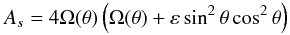 (10)and
  (11)so that
  (12)We assume that ε> −1 so that the Rayleigh stability criterion (As> 0 everywhere in the shell) is always satisfied. From Eq. (9), the slope of the paths of characteristics in the hyperbolic domain reads
  (13)where
 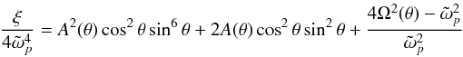 (14)and
 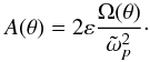 (15)As expected, all the above quantities and the dynamics of characteristics depend on θ alone.
3.2.2. Turning surfaces
 |
Fig. 1 Illustration of the two kinds of inertial modes propagating in a fluid with conical rotation profile Ω(θ) = Ω0(θ) / Ωref = 1 + εsin2θ, for m = { 0,1,2,4 }from top left to bottom right. The eigenfrequency in the inertial frame ωp is shown in x-axis and the differential rotation parameter ε is in y-axis. Blue: D modes that exist in the whole shell (ξ> 0 everywhere). White: DT modes that exhibit at least one turning surface inside the shell (the sign of ξ changes in the shell). Red: No inertial modes may exist in the shell (ξ< 0 everywhere). Orange: the modes in the region between the two orange lines feature a corotation layer ( |

In the set-up described in 3.2.1, ξ is symmetric about the equatorial plane of the shell so only values θ ∈ [ 0,π/ 2 ] need to be considered. As explained in the previous paragraph, equation ξ(θ) = 0 defines turning surfaces that separate the spherical shell into a hyperbolic domain (ξ> 0) and an elliptic domain (ξ< 0). Turning surfaces are portions of cones of axis z and aperture 2θ. However, their location cannot be determined analytically because ξ(θ) = 0 is a polynomial equation of degree 6 in X = sin2θ. Still their existence leads to two classes of inertial modes with conical rotation:
-
1.
modes for which at least one turning surface exists within the shell, referred to as DT modes following the terminology introduced in Baruteau & Rieutord (2013) (D for differential rotation, T for turning surface);
-
2.
modes that propagate in the whole shell, which is entirely hyperbolic because there is no turning surface within it, named D modes.
The occurrence of D and DT modes is depicted in Fig. 1 for the axisymmetric case (m = 0) and a few non-axisymmetric cases (m> 0). White areas represent DT modes which have ξ< 0 at least once within the shell, while blue regions represent D modes for which ξ> 0 everywhere within the shell. The red areas illustrate the case where ξ< 0 everywhere in the shell, for which the shell hosts no inertial modes. The curves that separate D and DT modes are implicitly defined by two equations:
-
ξ(θ = 0) = 0, which corresponds to the case where the turning surface is on the rotation axis, and which can be recast as
 (16)and is shown by the vertical dotted lines in Fig. 1;
 -
ξ(θ = π/ 2) = 0 when the turning surface reaches the equator, which yields
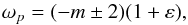 (17)and is shown by the solid black lines in Fig. 1.
We point out that there may be two turning surfaces in a meridional plane for a given set of parameters. For instance, in the bottom left panel of Fig. 1 (where m = 2), the transition from the central blue region to the white region around ωp = 0 shows that two turning surfaces occur at θ = π/ 4 before splitting towards the pole and the equator. Our investigations show that this only occurs for m = ± 2 around ωp = 0, which we checked by solving numerically the equation ξ(θ = π/ 4) = 0 for every m, whose solutions are depicted by the black dashed lines in Fig. 1. An example is given in the following subsection (see the bottom right panel of Fig. 5).
We note that for D modes – for which ∀θ,ξ(θ) > 0 – we have  , which means that for D modes, the standard criterion for propagation of inertial waves is met everywhere locally.
3.2.3. Critical layers
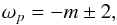
For non-axisymmetric modes (m ≠ 0),  may vanish in the shell, which corresponds to what are known as corotation resonances or critical layers (Baruteau & Rieutord 2013). Since is a function of θ only, a critical layer is the intersection of a cone of axis z with the spherical shell. As can be seen from Eq. (13), paths of characteristics may become locally vertical at corotation layers. Their location is given by
 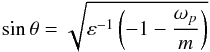 (18)and they exist only when ωp ∈ [−m, − m(1 + ε)] (if mε< 0) or when ωp ∈ [−m(1 + ε), −m] (if mε> 0). Critical layers exist for the D and DT modes located between the two orange lines in the panels of Fig. 1.
3.3. Dispersion relation, phase and group velocities
We expand the study of the propagation of inertial waves in the inviscid limit by considering the wave dispersion relation. This relation is obtained by assuming solutions to Eq. (7) in the form p ∝ exp [ i(kss + kzz) ] and adopting the short-wavelength approximation, ![Mathematical equation: \begin{equation} \tilde{\omega}_p^2 = \frac{k_z^2}{\| \vec{k} \|^2} \left[A_s - \frac{k_s}{k_z}A_z\right], \label{eq:dispersion_general} \end{equation}](/articles/aa/full_html/2016/05/aa27621-15/aa27621-15-eq112.png) (19)where
(19)where  . Assuming the bracket-term is positive, which is equivalent to assuming that the background rotation profile is dynamically stable to inertial waves (see the discussion in Sec. 2.1), we can define
 ![Mathematical equation: \begin{equation} \tilde{\mathcal{B}} = {\left[A_s - \frac{k_s}{k_z}A_z\right]}^{1/2} \end{equation}](/articles/aa/full_html/2016/05/aa27621-15/aa27621-15-eq114.png) (20)so that the wave dispersion becomes
(20)so that the wave dispersion becomes  . The phase and group velocities in a frame rotating with the fluid are then given by
 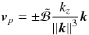 (21)and
 ![Mathematical equation: \begin{equation} \vec{v}_{g} = \pm \frac{k_s}{\left\|\vec{k}\right\|^3} \left(-k_z \vec{e}_{s} + k_s \vec{e}_{z} \right) \left[ \tilde{\mathcal{B}} +\frac{A_z}{2} \frac{\left\|\vec{k}\right\|^2}{k_s k_z} \tilde{\mathcal{B}}^{-1} \right], \end{equation}](/articles/aa/full_html/2016/05/aa27621-15/aa27621-15-eq117.png) (22)which corresponds to Eqs. (A9) and (A10) in \cite{BR2013}. We note that \begin{lxirformule}$\vec{k} \cdot \vec{v}_{g} = 0$\end{lxirformule} as for pure inertial waves propagating in a solid-body rotating fluid.
(22)which corresponds to Eqs. (A9) and (A10) in \cite{BR2013}. We note that \begin{lxirformule}$\vec{k} \cdot \vec{v}_{g} = 0$\end{lxirformule} as for pure inertial waves propagating in a solid-body rotating fluid.
Applying these formulae to our conical rotation profile Ω(θ) = 1 + εsin2θ, the dispersion relation is given by ![Mathematical equation: \begin{equation} \tilde{\omega}_p^2 = 4 \Omega^2(\theta) \frac{k_z^2}{\left\|\vec{k}\right\|^2}\left[ \left(1 + \frac{\varepsilon \sin^2 \theta \cos^2 \theta}{1+\varepsilon \sin^2 \theta}\right) +\frac{k_s}{k_z} \frac{\varepsilon \cos \theta \sin^3 \theta}{1+\varepsilon \sin^2 \theta} \right]\cdot \label{eq:dispersion} \end{equation}](/articles/aa/full_html/2016/05/aa27621-15/aa27621-15-eq119.png) (23)Assuming the fluid is stable against the GSF instability, we define
(23)Assuming the fluid is stable against the GSF instability, we define ![Mathematical equation: \begin{equation} \mathcal{B} = {\left[ \left(1 + \frac{\varepsilon \sin^2 \theta \cos^2 \theta}{1+\varepsilon \sin^2 \theta}\right) +\frac{k_s}{k_z} \frac{\varepsilon \cos \theta \sin^3 \theta}{1+\varepsilon \sin^2 \theta} \right]}^{1/2}, \end{equation}](/articles/aa/full_html/2016/05/aa27621-15/aa27621-15-eq120.png) (24)so that Eq. (23) becomes
(24)so that Eq. (23) becomes 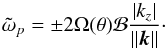 (25)For solid-body rotation, ℬ = 1 and Eq. (25) is the usual dispersion relation for inertial waves. Consequently, the phase velocity in the frame rotating with the fluid is
 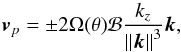 (26)while the group velocity is given by
 ![Mathematical equation: \begin{eqnarray} \vec{v}_{g} &=& \pm 2 \Omega(\theta) \frac{k_s}{\left\|\vec{k}\right\|^3} \left(-k_z \vec{e}_{s} + k_s \vec{e}_{z} \right) \nonumber\\ &&\times \left[ \mathcal{B} -\frac{2\Omega(\theta) \varepsilon \cos \theta \sin^3 \theta}{k_s k_z} \left\|\vec{k}\right\|^2 \mathcal{B}^{-1} \right]. \label{eq:group_velocity} \end{eqnarray}](/articles/aa/full_html/2016/05/aa27621-15/aa27621-15-eq124.png) (27)From Eq. (25), we see that a critical layer may form in the shell (
(27)From Eq. (25), we see that a critical layer may form in the shell ( ) in the following formal cases:
-
|ks| → ∞ at finite kz, so that vp = 0 and vg = 0 at corotation and inertial waves cannot cross critical layers;
-
|kz| → 0 at finite ks, so that vp = 0, vg·es = 0 and |vg·ez| → ∞, indicating that inertial waves may propagate across a critical layer with locally vertical paths of characteristics;
-
ℬ → 0, which implies again that vp = 0 while |vg·es| → ∞ and |vg·ez| → ∞, which means that in this case as well inertial waves may propagate across the corotation resonance with a finite slope for the paths of characteristics since ℬ = 0 implies
 (28)
(28)
3.4. Dynamics of the characteristics of inertial waves: attractor cycles, focusing points and Lyapunov exponents
 |
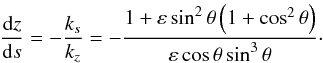
Fig. 2 Paths of characteristics for solid-body rotation (ε = 0). Left: paths of characteristics do not converge towards any periodic orbit (m = 0, ωp = 1.305, η = 0.35, and solid body-rotation ε = 0). Right: example of an attractor cycle of the path of characteristics for m = 2, ωp = −3.75, solid-body rotation (ε = 0), and the solar aspect ratio η = 0.71. |
In the case of solid-body rotation, the paths of characteristics in a meridional plane follow straight lines that form a constant angle with the rotation axis (i.e. the z-axis), which only depends on the uniform Doppler-shifted wavefrequency  (see the dispersion relation given in Eq. (25) for ε = 0). For a given aspect ratio of the shell η, certain values of the frequency ωp cause the paths of characteristics to converge towards periodic orbits called “attractors”, while for some other frequencies, paths of characteristics nearly occupy the whole shell with no obvious periodic pattern. These two different behaviours are illustrated in Fig. 2. The existence of one or several attractor(s) for a given set of parameters can be investigated by studying the exponential convergence rate of two close characteristics along multiple reflections. This is quantified by the Lyapunov exponent Λ (for more details, see Rieutord et al. 2001; Baruteau & Rieutord 2013). The Lyapunov exponent can be defined as
  (29)where dxk is the separation between two characteristics after k reflections. In our case, this quantity can be evaluated using either the reflections on the equator (dsk), on the rotation axis (dzk), or on the inner (resp. outer) boundary of the shell
  (resp.
  ). The value of Λ ≈ 0 corresponds to the case of “space-filling” paths of characteristics, whereas Λ < 0 identifies the existence of an attractor (see left and right panel of Fig. 2, respectively).
In the case of solid-body rotation, the locations where characteristics bounce off the shell spherical boundaries, the equator or the rotation axis, can be determined analytically, thus allowing for a semi-analytic calculation of Λ (Rieutord et al. 2001). However, differential rotation requires the numerical integration of the path of characteristics. For this purpose, we choose a starting point in the shell and we follow the propagation by numerically integrating Eq. (13). Since characteristics cannot propagate in the elliptic domain, it is necessary to impose reflection at turning surfaces.
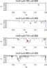 |
Fig. 3 Numerical spectrum of the Lyapunov exponent for m = 0, ε = 0.30, and ωp ∈ [ 0.2,2.0 ]. From top to bottom: η = { 0.10,0.35,0.71,0.90 }. The red open squares correspond to the modes shown in Figs. 6 to 8. |
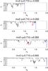 |
Fig. 4 Numerical spectrum of the Lyapunov exponent for m = 0, η = 0.71, and ωp ∈ [ 0.2,2.0 ]. From top to bottom: ε = { −0.50, −0.25,0.30,0.60 }. The blue solid line marks the frequency of the transition between the D and DT modes. The red open squares correspond to the modes shown in Figs. 6 to 8. |
For illustration purposes, we evaluated numerically the Lyapunov exponents as a function of the eigenfrequency for m = 0 for different values of η and ε:
-
η = { 0.10,0.35,0.71,0.90 } along with a fixed solar-like value of the differential rotation parameter ε = 0.30 for Fig. 3;
-
ε = { −0.50, −0.25,0.30,0.60 } along with a fixed solar-like value of the convective shell aspect ratio η = 0.71 for Fig. 4.
We used 800 frequencies per unit interval of frequencies and ten pairs of characteristics for each data point before averaging the results. The results shown in Figs. 3 and 4 should therefore be considered a qualitative indicator of the presence of short-period attractor cycles rather than a quantitative one because our method probably yields substantial uncertainties on the values of Λ. We also note that the focusing of characteristics towards a wedge in the frequency range of DT modes (see the bottom left panel of Fig. 5 below) prevented us from computing values of Λ for the DT modes. As expected, attractors of various strengths exist in small intervals of frequencies where Λ is strictly negative, whereas intervals where Λ ≈ 0 are associated with very long-period attractors or quasi-periodic orbits of characteristics.
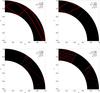 |
Fig. 5 Upper left: example of attractor cycle for a D mode with m = 2, ωp = −3.75 in a solar-like convective envelope (ε = 0.3, η = 0.71). Upper right: same for a DT mode with m = 0, frequency ωp = 1.68, and anti-solar conical rotation (ε = −0.3); the white dashed line shows the turning surface. Bottom left: illustration of the focusing of the paths of characteristics at the intersection of the turning surface (dashed line) and the outer boundary of the shell (m = 0, ωp = 2.4, and ε = 0.5). Bottom right: for m = 2, ωp = −0.126, and ε = −0.90 two turning surfaces exist within the shell, allowing the propagation of characteristics near the equator or the poles but not in between. |
Figure 3 illustrates how the existence of short-period attractors in the frequency range of inertial waves can be affected by the size of the inner core. It seems that when the core is small, attractors of characteristics are very rare but still exist as illustrated by the region around ωp ≈ 1.66 in the top left panel of Fig. 3. We checked that this attractor exists regardless of the size of the inner core as long as the latter is small enough, and we computed the corresponding eigenmode (see Fig. 8, and Fig. 8 in Baruteau & Rieutord 2013). However, the other panels of Fig. 3 indicate that more and more attractors exist with increasing values of η, owing to increasingly numerous reflections on the inner core. The case where η = 0.90 shows that a large number of short-period attractors exist over the frequency range of D modes.
Figure 4 shows the evolution of the Lyapunov exponent spectrum for a given core size, but for various values of the differential rotation parameter ε. We see that the occurrence of short-period attractors is not sensitive to ε, but some features of the Lyapunov spectra can be tracked as they are progressively altered and shifted to higher frequencies with increasing ε (e.g. the deep double peak starting from ωp ∈ [ 0.3,0.5 ] in the top left panel and shifted to ωp ∈ [ 1.25,1.5 ] in the bottom right panel).
When the fluid differentially rotates with angular velocity Ω(θ), paths of characteristics may still converge towards attractors – just like in the case of solid-body rotation – but with curved characteristics as illustrated in the top left panel of Fig. 5. They also depend on the azimuthal wavenumber m through the non-uniform Doppler-shifted frequency . We can also find attractors of characteristics when a turning surface exists in the shell (top right panel). Sometimes characteristics tend to focus at the intersection of a turning surface with the boundaries of the shell as illustrated by the bottom left plot of Fig. 5, showing a behaviour that is similar to the one found by Dintrans et al. (1999) for gravito-inertial waves. Finally, we note that in rare cases, two turning surfaces can exist within the shell, affecting the waves’ propagation domain accordingly: it is either restricted to the polar and equatorial regions (as illustrated in the bottom right panel of Fig. 5) or restricted to mid-latitudinal regions.
4. Viscous problem: shear layers, comparison to inviscid analysis, behaviour at corotation resonances
Our study of the propagation properties of inertial waves in a differentially rotating inviscid fluid with a conical rotation profile (see Sect. 3) shows that two families of inertial modes of oscillation exist: D modes that may propagate in the entire shell, and DT modes that are trapped in part of the shell because of the existence of a turning surface. We find that paths of characteristics depend on m through the Doppler-shifted wavefrequency, which is not the case for solid-body rotation, but the main difference between m = 0 and m ≠ 0 modes is the possible existence of corotation resonances in the latter case.
In Sect. 4.1, we briefly present the numerical method we used to solve the viscous problem exposed in Sect. 2.1. Then we study via numerical simulations in Sects. 4.2 and 4.3 respectively the general properties of weakly damped viscous D modes that propagate in the whole spherical shell and the DT modes that propagate in part of the shell. We show in particular how the shear layer structure can be related to the inviscid analysis detailed above in Sect. 3. As explained in the introduction of this work, we will mostly focus on singular modes for which a short-period attractor of characteristics exists since they may be related with strong viscous dissipation (Ogilvie 2005). Finally, we examine m ≠ 0 modes with corotation resonances in Sect. 4.4.
4.1. Numerical method
The linearized dimensionless system of Eqs. (6) and the associated stress-free boundary conditions are solved using a unique decomposition of the unknown velocity field u onto vectorial spherical harmonics (Rieutord 1987),  (30)with
  ,
,  , and
, and  , where
  is the usual spherical harmonic of degree l and order m normalized on the unit sphere, and ∇H = eθ∂θ + eϕ(sinθ)-1∂ϕ is the horizontal gradient.
The projection of the continuity equation on  gives
gives  as a simple function of
  and
and  . The momentum equation is then projected on
  and
and  , which yields two long ordinary differential equations involving only the radial functions and
  (since can be eliminated):
-
1.
the right-hand side of the second-order equation satisfied by
is a linear combination of  ,
,  ,
,  ,
,  , and
, and  (this term vanishes for m = 0);
 -
2.
the right-hand side of the fourth-order differential equation satisfied by
is a linear combination of  ,
,  ,
,  ,
,  ,
,  ,
,  , and
, and  (these last three terms vanish for m = 0).
The fact that the radial functions , , and with different azimuthal wavenumbers m are not coupled is a consequence of the axisymmetry of the background flow. The coupling between different latitudinal degrees (from l − 3 to l + 3) results from the choice of our specific conical rotation profile through the Coriolis acceleration terms.
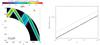 |
Fig. 6 Left: meridional cut of the normalized kinetic energy of an axisymmetric D mode with eigenfrequency ωp ≈ 1.15 obtained with E = 5 × 10⁻⁸, the Sun’s aspect ratio η = 0.71, and conical differential rotation ε = 0.3. The attractor of characteristics for these parameters is overplotted by the white curve. Right: scaling of the damping rate with respect to the Ekman number E. The dashed line is proportional to E1 / 3. |
In order to solve these equations numerically, they are discretized in the radial direction on the Gauss-Lobatto collocation nodes associated with Chebyshev polynomials. Each set of equations is truncated at order L for the spherical harmonics basis, and at order Nr for the Chebyshev basis. This yields a finite eigenvalue problem of order Nr × L with a block banded matrix composed of up to seven block bands. Then we use the linear solver based on the incomplete Arnoldi-Chebyshev algorithm (see details in Valdettaro et al. 2007) to compute pairs of eigenvalues (equal to iωp) and eigenvectors (values of , and on each point of the radial grid), given an initial value guess for iωp. Since the values of Nr and L required to achieve spectral convergence vary a lot from one mode to another, especially for the very demanding small values of E, some figures will be accompanied by the spectral content of the velocity field. In all the cases presented in this work we assumed symmetry with respect to the equatorial plane, which explains why our results are only shown for positive values of z, but anti-symmetry is also possible.
4.2. Axisymmetric and non-axisymmetric D modes with no corotation layer
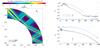 |
Fig. 7 Left: meridional cut of the normalized kinetic energy of a D mode with eigenfrequency ωp ≈ 1.355 obtained with E = 10-8 and anti-solar differential rotation ε = −0.25. The attractor of characteristics is overplotted by the thick white curve. Right: spectral content of the radial (u) and orthoradial (w) components of the velocity field for this mode. Chebyshev and spherical harmonics coefficients are shown in the top and bottom panels, respectively. |
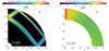 |
Fig. 8 Left: meridional cut of the normalized kinetic energy of a D mode with eigenfrequency ωp ≈ 1.66 obtained with E = 10-8, η = 0.10, and conical differential rotation ε = 0.30. The attractor of characteristics is again overplotted by the thick white curve. Right: meridional cut of the normalized kinetic energy of a D mode with eigenfrequency ωp ≈ 1.23 obtained with E = 10-8, η = 0.71, and conical differential rotation ε = −0.25. This mode is clearly associated with a quasi-periodic orbit of characteristics and not with an attractor. |
In this section we present our numerical results for a few representative D modes with a background conical rotation profile and Ekman numbers between 10-7 and 10-8, and we compare the structural properties of the shear layers with the inviscid analysis detailed in Sect. 3. We note that in the rest of this paper we always show the kinetic energy distribution of the computed velocity fields, but that the viscous dissipation looks qualitatively very similar (e.g. Fig. 13 in Baruteau & Rieutord 2013).
Figure 6 displays the result of one of our numerical calculations for an axisymmetric (m = 0) D mode with eigenfrequency ωp ≈ 0.91 obtained in a spherical shell of solar aspect ratio η = 0.71 with solar-like conical differential rotation (ε = 0.30). The left panel shows the spatial distribution of the mode’s kinetic energy in a meridional quarter-plane. The amplitude of the mode reaches its maximum near the rotation axis which is a feature shared by inertial modes in a uniformly rotating fluid shell. This has been demonstrated in detail in Appendix A of Rieutord & Valdettaro (1997) who showed that the kinetic energy along characteristic trajectories grows as s− 1 / 2 when s → 0. The structure of this specific mode mostly consists of a shear layer following a short-period attractor formed by slightly curved lines, as expected in the case of differential rotation (see Sect. 3). This attractor is overplotted with a thick white curve, which is the prediction for the propagation of characteristics under the short-wavelength approximation. The patterns formed by the attractor and by the shear layers of the viscous mode are in very good agreement. The mode shown in Fig. 6 was extracted from a sequence of calculations in which we followed a particular mode while progressively decreasing the Ekman number from 10-6 to 10-9. The damping rate of this mode is displayed as a function of E in the right panel of Fig. 6 where the dashed line clearly shows that it is proportional to E1 / 3, which is the scaling that is expected in the asymptotic regime for solid-body rotation (Rieutord & Valdettaro 1997), meaning that this kind of D mode is not deeply affected by differential rotation.
We show in Fig. 7 a qualitatively similar axisymmetric D mode of eigenfrequency ωp ≈ 1.35 that was obtained with the same aspect ratio but slightly lower Ekman number E = 10-8 and anti-solar differential rotation ε = −0.25. This time the amplitude of the mode still reaches its maximum at the rotation axis but is also quite large near the inner critical latitude (where the characteristics are tangent to the inner core), which is reminiscent of the solid-body rotation case where shear layers are sometimes emitted at the critical latitude. The right panel of Fig. 7 depicts the spectral content of u and w for this mode: the top panel shows the maximum Chebyshev coefficients Ck as a function of the Chebyshev order k, taking the highest value among all the spherical harmonics coefficients for a given k; similarly, the bottom panel shows the maximum spherical harmonics coefficients Cl as a function of the spherical harmonic degree: for a given l, we take the highest value among all the Chebyshev coefficients. Therefore, we are certain that numerical convergence is achieved for this mode.
Finally, the axisymmetric mode of frequency ωp ≈ 1.66 presented in the left panel of Fig. 8 displays a shear layer that follows an attractor of characteristics that exists for arbitrarily small values of the aspect ratio η. This means that in conical differential rotation, attractors of characteristics may exist independently of the existence of an inner core, which was also found for cylindrical and shellular differential rotation profiles by Baruteau & Rieutord (2013). We checked that this mode exists for arbitrarily small cores, which contrasts with the fact that inertial modes in a full sphere are regular in the case of solid-body rotation (Greenspan 1968; Zhang et al. 2001). Our result shows that this is probably no longer the case when differential rotation is taken into account. The case where characteristics do not converge towards any limit cycle is shown in the right-panel of Fig. 8, which displays a mode of frequency ωp ≈ 1.23 with η = 0.71 and ε = −0.25. This set of parameters corresponds to the open square in Fig. 4 for which Λ ≈ 0. As expected, the shear layer patterns visible here follow the propagation of characteristics so that the kinetic energy is more smoothly distributed than in the previous attractor cases.
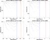 |
Fig. 9 Distribution of eigenvalues in the complex plane for m = 0 and E = 10-5 with a spectral resolution of Nr = 60 and L = 150. The top and bottom rows are for thick and thin shells (η = 0.35 and η = 0.71, respectively), while the left and right columns are for ε = 0.30 and ε = 0.60. In all panels, the vertical blue (resp. red) line depicts the transition between the frequency ranges of D and DT modes (resp. DT and non-existant modes). |
The four modes shown in Figs. 6 to 8 all correspond to one of the open squares in Figs. 3 and 4. This highlights the interest of the inviscid approach undertaken in Sect. 3 since the kinetic energy of a given mode is indeed more localized along thin shear layers when Λ < 0 and more uniformly-distributed in the shell when Λ ≈ 0. As a conclusion, the inviscid analysis allows us to understand how differential rotation affects inertial modes, although we restricted ourselves to D modes that can propagate in the whole spherical shell. We see that D modes behave quite similarly to inertial modes for solid-body rotation. In the next section we turn to DT modes, which are specific to differential rotation.
4.3. Axisymmetric and non-axisymmetric DT modes
In this section, we focus on modes for which a turning surface exists in the shell. The frequency range in which these modes can exist is indicated by the white areas in Fig. 1. However, not all sets of parameters falling in these white areas effectively correspond to an eigenmode. The inviscid analysis exposed in Sect. 3 reveals that characteristics cannot propagate in the elliptic domain of the shell, i.e. where ξ< 0 or equivalently  . As a consequence, for sufficiently small Ekman numbers, DT modes are expected to be trapped in the hyperbolic domain out of which characteristics cannot propagate, a property which has always been verified by our numerical calculations. We also present results in cases where characteristics converge towards the intersection of a turning surface with the inner or outer shell boundaries (see Fig. 5).
4.3.1. Existence of DT modes
In order to find DT modes, as a first step we checked the distribution of the eigenvalues of our linear problem for a given set of parameters, using a QZ factorization method. This method rapidly becomes very costly as the spectral resolution (and thus the dimensions of the linear problem) increases; therefore, we are limited to moderate values of E. Despite this limitation, trends are still discernable, especially with the sign of the differential rotation parameter ε.
Figure 9 shows our results for a few sets of parameters with solar rotation (ε> 0) that were obtained with a spectral resolution of Nr = 60 and L = 150. This resolution is usually sufficient to achieve spectral convergence for all the modes we computed at E = 10-5. We note that the eigenvalues with absolute damping rates above ~10-1 should be ignored because they are dominated by round-off errors and do not represent real resonant modes. We checked that the least damped eigenvalues located in the bottom part of each panel remained identical when slightly increasing or decreasing either Nr or L, while the most damped eigenvalues changed substantially – as was expected.
In all cases presented here the least damped modes are all D modes, whereas the potential DT modes have a much higher absolute damping rate and tend to be located near the boundaries of the DT-frequency range displayed by the blue and red lines. This emphasizes that it is numerically much more difficult to compute DT modes than D modes, as we have indeed experienced. We followed one of these potential DT modes, starting with an eigenfrequency close to the maximum frequency allowed for DT modes (i.e. the red line in Fig. 9) and decreasing the Ekman number from 10-5 to 10-9. We found that as E decreases, the eigenfrequency converges towards the maximum frequency. This frequency shift affects the location of the turning surface and therefore the size of the hyperbolic domain which simply disappears as E decreases. The very existence of this DT mode at lower Ekman numbers is therefore questionable.
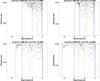 |
Fig. 11 Same as Fig. 9, but for m = 2 and solar aspect ratio η = 0.71. The four panels are for ε = { −0.50, −0.25,0.30,0.60 }. Orange solid lines are the boundaries of the frequency range in which a corotation layer exists inside the shell (see Fig. 1). Red symbols depict unstable eigenvalues for which Re(iωp) > 0. |
Our comment on Fig. 9 that could explain the rarity of DT modes is no longer valid in the case of anti-solar differential rotation presented in Fig. 10. Though most of the least damped modes are still D modes, some of them have frequencies that belong to the DT-frequency range, independently of the values of the parameters η and ε. This indicates that resonant axisymmetric DT modes in conical differential rotation mostly exist in the anti-solar case (ε< 0), which is consistent with our attempts to compute DT modes; this means that the QZ factorization method is a precious tool in the exploration of the different families of inertial modes.
As can be seen in Fig. 11, the trend indicating that resonant modes preferentially exist in the frequency range of D modes rather than of DT modes is still valid in the case of non-axisymmetric m = 2 modes. As explained in the introduction we chose m = 2 because it is the dominant non-axisymmetric component of the tidal potential. The red symbols depict unstable modes which surprisingly exist even at Ekman numbers as high as 10-5. All of them feature a critical layer inside the shell where the Doppler-shifted wavefrequency vanishes, which is reminiscent of the inviscid case exposed at the end of Sect. 3. We present our results of the non-axisymmetric modes with corotation resonances in Sect. 4.4.
4.3.2. Examples
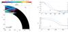 |
Fig. 12 Left: meridional cut of the normalized kinetic energy of a m = 0 DT mode with eigenfrequency ωp ≈ −1.86 obtained with E = 2.2 × 10⁻⁸, η = 0.71, and conical differential rotation ε = −0.25. The location of the turning surface is depicted by the white dashed line. Right: spectral content of the radial (u) and orthoradial (w) components of the velocity field for this mode. |
The axisymmetric DT mode presented in Fig. 12 was computed with η = 0.71 and anti-solar rotation parameter ε = −0.25. In order to do this we first computed a DT mode at eigenfrequency ωp ≈ 1.82 and Ekman number E = 10-5 before decreasing E step-by-step (typical steps being a relative change of a few per cent), using the eigenfrequency of a given step as an initial guess for the next step, along with increasing the spectral resolution. This method gives a better understanding of how the width of the shear layers and/or damping rates scale with E as we approach the astrophysically relevant regime of small E. As expected, the mode’s kinetic energy is restricted to the hyperbolic domain located near the rotation axis, and the shear layer emitted at the inner critical latitude indeed reflects on the white dashed line that represents the turning surface. Looking at the behaviour of the paths of characteristics for this set of parameters, we find that they eventually focus at the intersection of the inner core with the turning surface, as does the shear layer of the viscous mode.
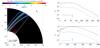 |
Fig. 13 Left: meridional cut of the normalized kinetic energy of a m = 2 DT mode with eigenfrequency ωp ≈ 3.22 obtained with E = 10-8, η = 0.35, and conical differential rotation ε = −0.43. The location of the turning surface is depicted by the white dashed line. Right: spectral content of the radial (u) and orthoradial (w) components of the velocity field for this mode. |
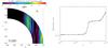 |
Fig. 14 Left: meridional cut of the normalized kinetic energy of an m = 2 D mode with eigenfrequency ωp ≈ −2.30 obtained with E = 10-9, the Sun’s aspect ratio η = 0.71, and conical differential rotation ε = 0.3. The corotation layer is overplotted by the red dashed line. Right: scaling of the damping rate with respect to the Ekman number E. A jump between two different modes is visible around E ≈ 7 × 10⁻⁸. |
Another interesting m = 2 DT mode is shown in Fig. 13 for ωp ≈ 3.22 and ε = −0.43. This mode features a shear layer that passes through both the inner and outer critical latitudes, and which focuses at the intersection between the inner core and the turning surface depicted by the white dashed line in the figure. We carefully checked that the paths of characteristics for these parameters indeed focus at this point.
4.4. Critical layers
The goal of this section is to show a few results of non-axisymmetric inertial modes for which a corotation layer exists in the shell, which in the case of our conical rotation profile is – by construction – a cone (see Eq. (18)). As pointed out at the end of Sect. 3, the fact that the Doppler-shifted wavefrequency vanishes has important consequences on the propagation properties of inertial waves, since it is a singularity of the inviscid problem. The wave phase velocity vp in the frame rotating with the fluid tends to zero at corotation while the group velocity may either tend to zero, have an infinite vertical component or have a finite slope in the case where ℬ = 0.
Figure 14 features a stable D mode obtained with high spectral resolution for m = 2 with ωp ≈ −2.30, solar parameters η = 0.71 and ε = 0.3, and E = 10-9. It was obtained by following a mode from E = 10-6 to E = 10-9. For these parameters, the corotation resonance is located at θ ≈ π/ 4 and is depicted by the red dashed line. A shear layer is emitted at the external critical latitude and the kinetic energy of the mode reaches its maximum there. The shear layer becomes more and more vertical as it approaches the corotation resonance, which is in agreement with the propagation properties of characteristics at that location. However, the corotation resonance does not seem to have any consequences other than a local energy accumulation around the critical layer. Unlike the axisymmetric D mode depicted in Fig. 6, the damping rate of this mode does not scale as a power of E, but seems to plateau to a constant value. The “jump” around E ≈ 7 × 10⁻⁸ occurs because our method always keeps the least damped mode at a given step and may therefore switch from one mode to another during the process. Put simply, it might just be an interaction with another eigenvalue.
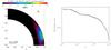 |
Fig. 15 Left: meridional cut of the normalized kinetic energy of an m = 2 D mode with eigenfrequency ωp ≈ −2.30 obtained with E = 10-9, the Sun’s aspect ratio η = 0.71, and conical differential rotation ε = 0.3. The corotation layer is overplotted by the red dashed line. Right: scaling of the growth rate with respect to the Ekman number E. A few jumps between different modes are visible around E ≈ {5 × 10-6,10-7,5 × 10⁻⁸}. |
The case of the mode depicted in Fig. 15 is different. We started from the unstable m = 2 D mode of eigenfrequency ωp ≈ −1.10 along with η = 0.71, ε = −0.5, and E = 10-5, which corresponds to the lowest red symbol in the top left panel of Fig. 11, and then progressively decreased E from 10-5 to 10-8 with a series of small steps. At each step, we used the eigenfrequency and damping rate of the previous step as the initial guess and selected the least damped (or most unstable) mode. The left panel of Fig. 15 displays a cut of the kinetic energy of the unstable velocity field obtained for E = 10-8. Unlike all the stable oscillation modes presented so far, it shows no recognizable shear layer structure. Instead, a patch of kinetic energy shows up around the location of the critical layer depicted by the red dashed line. The dependance of the growth rate of this particular mode with the Ekman number shown in the right panel also clearly differs from the classical E1 / 3-scaling presented in Fig. 7 for D modes, and is not even a power law. If we ignore the jumps between different modes (around E = 10-7 for instance), it seems that for a small enough E, the growth rate becomes roughly constant and reaches a very large value.
The role of critical layers in the propagation properties of different kinds of waves in various containers has been studied before in the fluid mechanics literature; for instance, Grimshaw (1979) studied the effect of critical levels on linear wave propagation as well as the associated absorption (Booker & Bretherton 1967) and valve effects (Acheson 1972, 1973). However, these works were restricted to the case where the mean flow is sheared in the vertical direction while our differential rotation profile is sheared in the horizontal direction. Using a different approach, Watson (1981) studied the stability of a conical rotation profile similar to ours with respect to non-axisymmetric wavelike perturbations, but was restricted to the case of two-dimensional Rossby waves with negligible radial velocity.
Nevertheless, it seems that critical layers can play a prominent role in the energy and momentum exchanges between the mean background flow and the waves velocity fields and may also strongly affect viscous dissipation. In order to understand the behaviour of inertial waves at corotation resonances, an interesting approach would be the study of a local one-dimensional model in which an inertial wave meets a critical layer induced by a horizontal shear in the background flow. This study is beyond the scope of this paper and is postponed to future work.
5. Conclusions and perspectives
In this work, we investigated the impact of conical differential rotation on the properties of free inertial waves in a homogeneous fluid inside a spherical shell container. This study is motivated by the possible important role of tidally driven inertial waves in the dynamical evolution of close star-planet or stellar binary systems.
First, we found that differential rotation implies different families of inertial waves and that the frequency range in which they exist can be broadened substantially compared to the solid-body rotation case, provided that a large enough latitudinal differential rotation exists in the convective envelopes of low-mass stars (Brun & Toomre 2002; Brown et al. 2008; Matt et al. 2011). We also showed that the D mode regime for which waves can propagate in the entire shell is essentially similar to the solid-body rotation case: wave attractors (which follow curved paths of characteristics) still exist in narrow frequency ranges (whose number increases with the size of the inner core, see Sect. 3) and viscous D modes seem to follow the same scaling relations with Ekman number. Moreover, the least damped modes seem to be found preferentially in the D mode frequency range. In addition, differential rotation also affects their allowed propagation domain: in the DT regime, modes are trapped around the poles or the equator by a turning surface. It seems, however, that resonant DT modes are rare especially for solar-like differential rotation. It is important to note that these conclusions only stand for axisymmetric modes or non-axisymmetric modes without corotation resonances. Indeed, we found that these corotation layers strongly modify the behaviour of inertial waves since the wave phase velocity always vanishes there, and the paths of characteristics and the associated viscous shear layers may become vertical while crossing the resonance. Among all the numerical calculations performed in the viscous case, we mostly found stable modes, but we also found several unstable modes at Ekman numbers as high as 10-5 which all featured a corotation resonance. As discussed when introducing the physics of the model, these unstable modes delineate the range of allowed parameters, since the background flow needs to be stable.
From the astrophysical perspective, these conclusions could have important dynamical implications for systems where inertial waves are excited, sustained and finally dissipated in a low-mass star with a latitudinal gradient of differential rotation in its convective envelope. One possible source of this excitation is tides raised by a close-in stellar or planetary companion. This requires that one or more of the components of the tidal potential, which depends on the orbital configuration of the system, has a frequency that falls in the inertial range with a high enough amplitude so that the kinetic energy stored by inertial oscillations and the subsequent viscous dissipation alters the orbital and rotational dynamics of the system. In a subsequent paper, we shall derive analytically the forcing term due to tides before computing numerically the velocity field and viscous dissipation of such tidally excited inertial waves. This will allow us to investigate the influence of differential rotation (e.g. through turning surfaces, corotation layers) in the convective envelope of low-mass stars on tidal dissipation for various parameters related to stellar mass, rotation, companion mass, and orbital parameters.
Finally, we point out the limitations and possible improvements of our work. In addition to the conditions of stability that we already mentioned, we note that our model only accounts for the direct effects of the viscous dissipation of inertial waves in convective envelopes, which may not be the only mechanism responsible for tidal dissipation – the non-linear breaking of gravity waves in the radiative interior is another mechanism, see Barker & Ogilvie (2010, 2011), Barker (2011) – especially in cases where these waves are likely not to be excited. Additionally, we point out that our study assumes the fluid to be incompressible and does not include the effects of non-linearities (see Jouve & Ogilvie 2014; Favier et al. 2014), which could become important for tidal oscillations of high amplitude, or the effects other processes that could affect the very nature of the low-frequency oscillations studied here, such as the magnetic field, the centrifugal distortion (Braviner & Ogilvie 2014; Barker & Lithwick 2014), or the possible interactions with turbulent convective motions (Ogilvie & Lesur 2012). However, the effects of differential rotation on the physical processes driving tidal dissipation have not yet been investigated, making this work a step towards a more detailed understanding of binary systems and star-planet interactions.
Acknowledgments
We warmly thank the referee A. J. Barker for his constructive comments which allowed us to improve the paper. M. Guenel and S. Mathis acknowledge funding by the European Research Council through ERC grant SPIRE 647383. This work was also supported by the Programme National de Planétologie (CNRS/INSU) and CNES PLATO grant at CEA-Saclay.
References
- Acheson, D. J. 1972, J. Fluid Mech., 53, 401 [NASA ADS] [CrossRef] [Google Scholar]
- Acheson, D. J. 1973, J. Fluid Mech., 58, 27 [NASA ADS] [CrossRef] [Google Scholar]
- Albrecht, S., Winn, J. N., Johnson, J. A., et al. 2012, ApJ, 757, 18 [NASA ADS] [CrossRef] [Google Scholar]
- Barker, A. J. 2011, MNRAS, 414, 1365 [NASA ADS] [CrossRef] [Google Scholar]
- Barker, A. J., & Lithwick, Y. 2014, MNRAS, 437, 305 [NASA ADS] [CrossRef] [Google Scholar]
- Barker, A. J., & Ogilvie, G. I. 2009, MNRAS, 395, 2268 [NASA ADS] [CrossRef] [Google Scholar]
- Barker, A. J., & Ogilvie, G. I. 2010, MNRAS, 404, 1849 [NASA ADS] [Google Scholar]
- Barker, A. J., & Ogilvie, G. I. 2011, MNRAS, 417, 745 [NASA ADS] [CrossRef] [Google Scholar]
- Baruteau, C., & Rieutord, M. 2013, J. Fluid Mech., 719, 47 [Google Scholar]
- Baruteau, C., Crida, A., Paardekooper, S.-J., et al. 2014, Protostars and Planets VI, 667 [Google Scholar]
- Booker, J. R., & Bretherton, F. P. 1967, J. Fluid Mech., 27, 513 [NASA ADS] [CrossRef] [Google Scholar]
- Braviner, H. J., & Ogilvie, G. I. 2014, MNRAS, 441, 2321 [NASA ADS] [CrossRef] [Google Scholar]
- Brown, B. P., Browning, M. K., Brun, A. S., Miesch, M. S., & Toomre, J. 2008, ApJ, 689, 1354 [CrossRef] [Google Scholar]
- Brun, A. S., & Toomre, J. 2002, ApJ, 570, 865 [NASA ADS] [CrossRef] [EDP Sciences] [Google Scholar]
- Bryan, G. H. 1889, Roy. Soc. London Philos. Trans. Ser. A, 180, 187 [Google Scholar]
- Cartan, E. 1922, Bull. Sci. Math., 46, 317 [Google Scholar]
- Chatterjee, S., Ford, E. B., Matsumura, S., & Rasio, F. A. 2008, ApJ, 686, 580 [NASA ADS] [CrossRef] [Google Scholar]
- Damiani, C., & Lanza, A. F. 2015, A&A, 574, A39 [NASA ADS] [CrossRef] [EDP Sciences] [Google Scholar]
- Dintrans, B., Rieutord, M., & Valdettaro, L. 1999, J. Fluid Mech., 398, 271 [NASA ADS] [CrossRef] [Google Scholar]
- Favier, B., Barker, A. J., Baruteau, C., & Ogilvie, G. I. 2014, MNRAS, 439, 845 [NASA ADS] [CrossRef] [Google Scholar]
- Friedlander, S. 1982, Geophys. Astrophys. Fluid Dynam., 21, 189 [NASA ADS] [CrossRef] [Google Scholar]
- García, R. A., Turck-Chièze, S., Jiménez-Reyes, S. J., et al. 2007, Science, 316, 1591 [NASA ADS] [CrossRef] [PubMed] [Google Scholar]
- Gastine, T., Yadav, R. K., Morin, J., Reiners, A., & Wicht, J. 2014, MNRAS, 438, L76 [NASA ADS] [CrossRef] [Google Scholar]
- Giuricin, G., Mardirossian, F., & Mezzetti, M. 1984, A&A, 134, 365 [Google Scholar]
- Goldreich, P., & Keeley, D. A. 1977, ApJ, 211, 934 [NASA ADS] [CrossRef] [Google Scholar]
- Goldreich, P., & Nicholson, P. D. 1989, ApJ, 342, 1079 [NASA ADS] [CrossRef] [Google Scholar]
- Goodman, J., & Dickson, E. S. 1998, ApJ, 507, 938 [NASA ADS] [CrossRef] [Google Scholar]
- Goodman, J., & Lackner, C. 2009, ApJ, 696, 2054 [NASA ADS] [CrossRef] [Google Scholar]
- Greenspan, H. P. 1968, The theory of rotating fluids (Cambridge University Press) [Google Scholar]
- Grimshaw, R. 1979, Geophys. Astrophys. Fluid Dynam., 14, 303 [NASA ADS] [CrossRef] [Google Scholar]
- Guillot, T., Lin, D. N. C., Morel, P., Havel, M., & Parmentier, V. 2014, in EAS PS, 65, 327 [Google Scholar]
- Hansen, B. M. S. 2010, ApJ, 723, 285 [NASA ADS] [CrossRef] [Google Scholar]
- Husnoo, N., Pont, F., Mazeh, T., et al. 2012, MNRAS, 422, 3151 [NASA ADS] [CrossRef] [Google Scholar]
- Hut, P. 1980, A&A, 92, 167 [NASA ADS] [Google Scholar]
- Jackson, B., Greenberg, R., & Barnes, R. 2008, ApJ, 678, 1396 [NASA ADS] [CrossRef] [Google Scholar]
- Jouve, L., & Ogilvie, G. I. 2014, J. Fluid Mech., 745, 223 [Google Scholar]
- Lai, D. 2012, MNRAS, 423, 486 [NASA ADS] [CrossRef] [Google Scholar]
- Le Bars, M., Cébron, D., & Le Gal, P. 2015, Ann. Rev. Fluid Mech., 47, 163 [NASA ADS] [CrossRef] [Google Scholar]
- Maas, L. R. M., & Lam, F.-P. A. 1995, J. Fluid Mech., 300, 1 [NASA ADS] [CrossRef] [Google Scholar]
- Mathis, S. 2015, A&A, 580, L3 [Google Scholar]
- Mathis, S., & Remus, F. 2013, in Lect. Not. Phys., 857, eds. J.-P. Rozelot, & C. Neiner (Berlin: Springer Verlag), 111 [Google Scholar]
- Matt, S. P., Do Cao, O., Brown, B. P., & Brun, A. S. 2011, Astron. Nachr., 332, 897 [NASA ADS] [CrossRef] [Google Scholar]
- Mazeh, T., Perets, H. B., McQuillan, A., & Goldstein, E. S. 2015, ApJ, 801, 3 [NASA ADS] [CrossRef] [Google Scholar]
- Meibom, S., & Mathieu, R. D. 2005, ApJ, 620, 970 [NASA ADS] [CrossRef] [Google Scholar]
- Meibom, S., Mathieu, R. D., & Stassun, K. G. 2006, ApJ, 653, 621 [NASA ADS] [CrossRef] [Google Scholar]
- Miesch, M. S., Brun, A. S., De Rosa, M. L., & Toomre, J. 2008, ApJ, 673, 557 [NASA ADS] [CrossRef] [Google Scholar]
- Naoz, S., Farr, W. M., Lithwick, Y., Rasio, F. A., & Teyssandier, J. 2011, Nature, 473, 187 [NASA ADS] [CrossRef] [Google Scholar]
- Ogilvie, G. I. 2005, J. Fluid Mech., 543, 19 [NASA ADS] [CrossRef] [Google Scholar]
- Ogilvie, G. I. 2009, MNRAS, 396, 794 [NASA ADS] [CrossRef] [Google Scholar]
- Ogilvie, G. I. 2013, MNRAS, 429, 613 [NASA ADS] [CrossRef] [Google Scholar]
- Ogilvie, G. I. 2014, ARA&A, 52, 171 [Google Scholar]
- Ogilvie, G. I., & Lesur, G. 2012, MNRAS, 422, 1975 [NASA ADS] [CrossRef] [Google Scholar]
- Ogilvie, G. I., & Lin, D. N. C. 2004, ApJ, 610, 477 [NASA ADS] [CrossRef] [Google Scholar]
- Ogilvie, G. I., & Lin, D. N. C. 2007, ApJ, 661, 1180 [NASA ADS] [CrossRef] [Google Scholar]
- Papaloizou, J. C. B., & Savonije, G. J. 1997, MNRAS, 291, 651 [NASA ADS] [CrossRef] [Google Scholar]
- Penev, K., Jackson, B., Spada, F., & Thom, N. 2012, ApJ, 751, 96 [NASA ADS] [CrossRef] [Google Scholar]
- Poincaré, H. 1885, Acta Math., 7, 259 [CrossRef] [MathSciNet] [Google Scholar]
- Pont, F. 2009, MNRAS, 396, 1789 [NASA ADS] [CrossRef] [Google Scholar]
- Rieutord, M. 1987, Geophys. Astrophys. Fluid Dynam., 39, 163 [Google Scholar]
- Rieutord, M., & Valdettaro, L. 1997, J. Fluid Mech., 341, 77 [NASA ADS] [CrossRef] [Google Scholar]
- Rieutord, M., & Valdettaro, L. 2010, J. Fluid Mech., 643, 363 [NASA ADS] [CrossRef] [Google Scholar]
- Rieutord, M., Georgeot, B., & Valdettaro, L. 2001, J. Fluid Mech., 435, 103 [NASA ADS] [CrossRef] [Google Scholar]
- Rocca, A. 1987, A&A, 175, 81 [Google Scholar]
- Rocca, A. 1989, A&A, 213, 114 [NASA ADS] [Google Scholar]
- Savonije, G. J., & Papaloizou, J. C. B. 1983, MNRAS, 203, 581 [NASA ADS] [CrossRef] [Google Scholar]
- Savonije, G. J., & Papaloizou, J. C. B. 1984, MNRAS, 207, 685 [NASA ADS] [CrossRef] [Google Scholar]
- Savonije, G. J., & Papaloizou, J. C. B. 1997, MNRAS, 291, 633 [Google Scholar]
- Savonije, G. J., Papaloizou, J. C. B., & Alberts, F. 1995, MNRAS, 277, 471 [NASA ADS] [CrossRef] [Google Scholar]
- Schou, J., Antia, H. M., Basu, S., et al. 1998, ApJ, 505, 390 [NASA ADS] [CrossRef] [Google Scholar]
- Strugarek, A., Brun, A. S., Matt, S. P., & Réville, V. 2014, ApJ, 795, 86 [NASA ADS] [CrossRef] [Google Scholar]
- Terquem, C., Papaloizou, J. C. B., Nelson, R. P., & Lin, D. N. C. 1998, ApJ, 502, 788 [NASA ADS] [CrossRef] [Google Scholar]
- Thomson, S. W. 1880, Philosophical Magazine Series 5, 10, 155 [Google Scholar]
- Valdettaro, L., Rieutord, M., Braconnier, T., & Fraysse, V. 2007, J. Comp. Appl. Math., 205, 382 [Google Scholar]
- Verbunt, F., & Phinney, E. S. 1995, A&A, 296, 709 [NASA ADS] [Google Scholar]
- Watson, M. 1981, Geophys. Astrophys. Fluid Dynam., 16, 285 [Google Scholar]
- Winn, J. N., Fabrycky, D., Albrecht, S., & Johnson, J. A. 2010, ApJ, 718, L145 [NASA ADS] [CrossRef] [Google Scholar]
- Witte, M. G., & Savonije, G. J. 1999, A&A, 350, 129 [NASA ADS] [Google Scholar]
- Witte, M. G., & Savonije, G. J. 2001, A&A, 366, 840 [NASA ADS] [CrossRef] [EDP Sciences] [Google Scholar]
- Witte, M. G., & Savonije, G. J. 2002, A&A, 386, 222 [NASA ADS] [CrossRef] [EDP Sciences] [Google Scholar]
- Zahn, J. P. 1966a, Annales d’Astrophysique, 29, 313 [Google Scholar]
- Zahn, J. P. 1966b, Annales d’Astrophysique, 29, 489 [Google Scholar]
- Zahn, J.-P. 1975, A&A, 41, 329 [NASA ADS] [Google Scholar]
- Zahn, J.-P. 1977, A&A, 57, 383 [NASA ADS] [Google Scholar]
- Zahn, J.-P. 2013, in Lect. Notes Phys. 861, eds. J. Souchay, S. Mathis, & T. Tokieda, (Berlin: Springer Verlag), 301 [Google Scholar]
- Zhang, K., Earnshaw, P., Liao, X., & Busse, F. H. 2001, J. Fluid Mech., 437, 103 [NASA ADS] [CrossRef] [Google Scholar]
All Figures
|
Fig. 1 Illustration of the two kinds of inertial modes propagating in a fluid with conical rotation profile Ω(θ) = Ω0(θ) / Ωref = 1 + εsin2θ, for m = { 0,1,2,4 }from top left to bottom right. The eigenfrequency in the inertial frame ωp is shown in x-axis and the differential rotation parameter ε is in y-axis. Blue: D modes that exist in the whole shell (ξ> 0 everywhere). White: DT modes that exhibit at least one turning surface inside the shell (the sign of ξ changes in the shell). Red: No inertial modes may exist in the shell (ξ< 0 everywhere). Orange: the modes in the region between the two orange lines feature a corotation layer ( |
| In the text | |
|
Fig. 2 Paths of characteristics for solid-body rotation (ε = 0). Left: paths of characteristics do not converge towards any periodic orbit (m = 0, ωp = 1.305, η = 0.35, and solid body-rotation ε = 0). Right: example of an attractor cycle of the path of characteristics for m = 2, ωp = −3.75, solid-body rotation (ε = 0), and the solar aspect ratio η = 0.71. |
| In the text | |
|
Fig. 3 Numerical spectrum of the Lyapunov exponent for m = 0, ε = 0.30, and ωp ∈ [ 0.2,2.0 ]. From top to bottom: η = { 0.10,0.35,0.71,0.90 }. The red open squares correspond to the modes shown in Figs. 6 to 8. |
| In the text | |
|
Fig. 4 Numerical spectrum of the Lyapunov exponent for m = 0, η = 0.71, and ωp ∈ [ 0.2,2.0 ]. From top to bottom: ε = { −0.50, −0.25,0.30,0.60 }. The blue solid line marks the frequency of the transition between the D and DT modes. The red open squares correspond to the modes shown in Figs. 6 to 8. |
| In the text | |
|
Fig. 5 Upper left: example of attractor cycle for a D mode with m = 2, ωp = −3.75 in a solar-like convective envelope (ε = 0.3, η = 0.71). Upper right: same for a DT mode with m = 0, frequency ωp = 1.68, and anti-solar conical rotation (ε = −0.3); the white dashed line shows the turning surface. Bottom left: illustration of the focusing of the paths of characteristics at the intersection of the turning surface (dashed line) and the outer boundary of the shell (m = 0, ωp = 2.4, and ε = 0.5). Bottom right: for m = 2, ωp = −0.126, and ε = −0.90 two turning surfaces exist within the shell, allowing the propagation of characteristics near the equator or the poles but not in between. |
| In the text | |
|
Fig. 6 Left: meridional cut of the normalized kinetic energy of an axisymmetric D mode with eigenfrequency ωp ≈ 1.15 obtained with E = 5 × 10⁻⁸, the Sun’s aspect ratio η = 0.71, and conical differential rotation ε = 0.3. The attractor of characteristics for these parameters is overplotted by the white curve. Right: scaling of the damping rate with respect to the Ekman number E. The dashed line is proportional to E1 / 3. |
| In the text | |
|
Fig. 7 Left: meridional cut of the normalized kinetic energy of a D mode with eigenfrequency ωp ≈ 1.355 obtained with E = 10-8 and anti-solar differential rotation ε = −0.25. The attractor of characteristics is overplotted by the thick white curve. Right: spectral content of the radial (u) and orthoradial (w) components of the velocity field for this mode. Chebyshev and spherical harmonics coefficients are shown in the top and bottom panels, respectively. |
| In the text | |
|
Fig. 8 Left: meridional cut of the normalized kinetic energy of a D mode with eigenfrequency ωp ≈ 1.66 obtained with E = 10-8, η = 0.10, and conical differential rotation ε = 0.30. The attractor of characteristics is again overplotted by the thick white curve. Right: meridional cut of the normalized kinetic energy of a D mode with eigenfrequency ωp ≈ 1.23 obtained with E = 10-8, η = 0.71, and conical differential rotation ε = −0.25. This mode is clearly associated with a quasi-periodic orbit of characteristics and not with an attractor. |
| In the text | |
|
Fig. 9 Distribution of eigenvalues in the complex plane for m = 0 and E = 10-5 with a spectral resolution of Nr = 60 and L = 150. The top and bottom rows are for thick and thin shells (η = 0.35 and η = 0.71, respectively), while the left and right columns are for ε = 0.30 and ε = 0.60. In all panels, the vertical blue (resp. red) line depicts the transition between the frequency ranges of D and DT modes (resp. DT and non-existant modes). |
| In the text | |
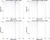 |
Fig. 10 Same as Fig. 9 except that the left and right columns are for ε = −0.25 and ε = −0.50. |
| In the text | |
|
Fig. 11 Same as Fig. 9, but for m = 2 and solar aspect ratio η = 0.71. The four panels are for ε = { −0.50, −0.25,0.30,0.60 }. Orange solid lines are the boundaries of the frequency range in which a corotation layer exists inside the shell (see Fig. 1). Red symbols depict unstable eigenvalues for which Re(iωp) > 0. |
| In the text | |
|
Fig. 12 Left: meridional cut of the normalized kinetic energy of a m = 0 DT mode with eigenfrequency ωp ≈ −1.86 obtained with E = 2.2 × 10⁻⁸, η = 0.71, and conical differential rotation ε = −0.25. The location of the turning surface is depicted by the white dashed line. Right: spectral content of the radial (u) and orthoradial (w) components of the velocity field for this mode. |
| In the text | |
|
Fig. 13 Left: meridional cut of the normalized kinetic energy of a m = 2 DT mode with eigenfrequency ωp ≈ 3.22 obtained with E = 10-8, η = 0.35, and conical differential rotation ε = −0.43. The location of the turning surface is depicted by the white dashed line. Right: spectral content of the radial (u) and orthoradial (w) components of the velocity field for this mode. |
| In the text | |
|
Fig. 14 Left: meridional cut of the normalized kinetic energy of an m = 2 D mode with eigenfrequency ωp ≈ −2.30 obtained with E = 10-9, the Sun’s aspect ratio η = 0.71, and conical differential rotation ε = 0.3. The corotation layer is overplotted by the red dashed line. Right: scaling of the damping rate with respect to the Ekman number E. A jump between two different modes is visible around E ≈ 7 × 10⁻⁸. |
| In the text | |
|
Fig. 15 Left: meridional cut of the normalized kinetic energy of an m = 2 D mode with eigenfrequency ωp ≈ −2.30 obtained with E = 10-9, the Sun’s aspect ratio η = 0.71, and conical differential rotation ε = 0.3. The corotation layer is overplotted by the red dashed line. Right: scaling of the growth rate with respect to the Ekman number E. A few jumps between different modes are visible around E ≈ {5 × 10-6,10-7,5 × 10⁻⁸}. |
| In the text | |
Current usage metrics show cumulative count of Article Views (full-text article views including HTML views, PDF and ePub downloads, according to the available data) and Abstracts Views on Vision4Press platform.
Data correspond to usage on the plateform after 2015. The current usage metrics is available 48-96 hours after online publication and is updated daily on week days.
Initial download of the metrics may take a while.