| Issue |
A&A
Volume 589, May 2016
|
|
|---|---|---|
| Article Number | A73 | |
| Number of page(s) | 8 | |
| Section | Galactic structure, stellar clusters and populations | |
| DOI | https://doi.org/10.1051/0004-6361/201527570 | |
| Published online | 14 April 2016 | |
MILES extended: Stellar population synthesis models from the optical to the infrared
1
Instituto de Astrofísica de Canarias,
Vía Láctea s/n, 38205 La Laguna,
Tenerife,
Spain
e-mail:
benny.roeck@gmail.com
2
Departamento de Astrofísica, Universidad de La
Laguna, 38205, La
Laguna, Tenerife,
Spain
3
Departament d’Astronomia i Astrofisica, Universitat de
Valencia, c/Dr. Moliner 50, 46100
Burjassot, Valencia, Spain
4
Kapteyn Astronomical Institute, University of
Groningen, Postbus
800, 9700 AV
Groningen, The
Netherlands
Received: 15 October 2015
Accepted: 25 February 2016
We present the first single-burst stellar population models, which covers the optical and the infrared wavelength range between 3500 and 50 000 Å and which are exclusively based on empirical stellar spectra. To obtain these joint models, we combined the extended MILES models in the optical with our new infrared models that are based on the IRTF (Infrared Telescope Facility) library. The latter are available only for a limited range in terms of both age and metallicity. Our combined single-burst stellar population models were calculated for ages larger than 1 Gyr, for metallicities between [ Fe / H ] = − 0.40 and 0.26, for initial mass functions of various types and slopes, and on the basis of two different sets of isochrones. They are available to the scientific community on the MILES web page. We checked the internal consistency of our models and compared their colour predictions to those of other models that are available in the literature. Optical and near infrared colours that are measured from our models are found to reproduce the colours well that were observed for various samples of early-type galaxies. Our models will enable a detailed analysis of the stellar populations of observed galaxies.
Key words: infrared: stars / infrared: galaxies / galaxies: stellar content
© ESO, 2016
Properties of our combined model SSP SEDs.
1. Introduction
Single-burst stellar population (SSP) models mimic uniform stellar populations of fixed age and metallicity, and are an important tool to study unresolved stellar clusters and galaxies. They are created by populating theoretical stellar evolutionary tracks with stars of a stellar library, according to a prescription given by a chosen initial mass function (IMF). Thus, the quality of the resulting SSP models depends significantly on the completeness of the used input stellar library in terms of evolutionary phases represented by the atmospheric parameters temperature, Teff, surface gravity, log (g), and metallicity. A sufficiently large spectral coverage is equally crucial when constructing reasonable SSP models. Theoretical stellar libraries like, e.g. BaSeL (Kurucz 1992; Lejeune et al. 1997, 1998; Westera et al. 2002), or PHOENIX (Allard et al. 2012; Husser et al. 2013) are generally available for both a large range in wavelength and in stellar parameters, whereas empirical libraries are found to be more incomplete in both respects. However, the advantage of the latter ones is that they are not hampered by the still large uncertainties in the calculation of model atmospheres. Examples of empirical stellar libraries in the optical wavelenth range encompass the Pickles library (Pickles 1998), ELODIE (Prugniel & Soubiran 2001), STELIB (Le Borgne et al. 2003), Indo-US (Valdes et al. 2004), MILES (Sánchez-Blázquez et al. 2006), and CaT (Cenarro et al. 2001, 2007). In the near-infrared (NIR) and mid-infrared (MIR)1, only very few empirical libraries have been observed so far (e.g. Lançon & Wood 2000; Cushing et al. 2005; Rayner et al. 2009). The NASA Infrared Telescope Facility (IRTF) spectral library, described in the latter two papers, is to date the only empirical stellar library in the NIR and MIR which offers a sufficiently complete coverage of the stellar atmospheric parameter space to construct SSP models. In the future, the X-Shooter stellar library, which contains around 700 stars, and which covers the whole optical (see Chen et al. 2014) and NIR wavelength range until 2.5 μm, will clearly improve the current situation in the NIR.
In the optical range, many different sets of SSP models have been developed, based on the abovementioned libraries (e.g. Worthey 1994; Vazdekis 1999; Bruzual & Charlot 2003; Le Borgne et al. 2004; Maraston 2005; Maraston et al. 2009; Conroy et al. 2009; Vazdekis et al. 2010). Other models cover the NIR and MIR ranges, like those by Maraston (2005), Conroy & van Dokkum (2012), Meneses-Goytia et al. (2015b), and Röck et al. (2015, hereafter R15).
In the current work, we combine our IRTF-based SSP models in the NIR and MIR with the MIUSCAT models (Vazdekis et al. 2012; Ricciardelli et al. 2012) in the optical range. Thus we end up with combined SSP models, which are based on empirical stellar spectral libraries and encompass the spectral range from 3465 to 50 000 Å. Moreover, we analyse and validate our new models in the NIR wavelength range between 1 and 2.5 μm.
2. Models from the optical to the infrared
In this section, we describe how we combined the MIUSCAT models (Vazdekis et al. 2012), which range from 3465 to 9469 Å, with our newly developed SSP models in the NIR and MIR (R15). We briefly recall the main ingredients and characteristics of the models in the two spectral ranges. A more detailed explanation of the modelling procedure is given in Vazdekis et al. (2003), Vazdekis et al. (2010, 2012, hereafter V10, V12) for the optical and in R15 for the IR part of the models.
2.1. Main ingredients and characteristics
Both the MIUSCAT models in the optical wavelength range and the IRTF-based models in the IR were calculated based on the isochrones of Girardi et al. (2000; hereafter Padova00 isochrones) and on those of Pietrinferni et al. (2004; BaSTI isochrones). All of our used sets of isochrones are scaled-solar ones.
It is important to note that the MIUSCAT models (V12) themselves are a compilation based on three different stellar libraries. The main part – from 3525 to 7410 Å – consists of the MILES stellar library (V10), whereas bluewards and redwards of it the Indo-US spectral library (Valdes et al. 2004) and the CaT one (Vazdekis et al. 2003) were used in order to extend the total spectral range coverage.
Whereas the MIUSCAT models are also available for young ages between 0.03 and 1 Gyr (BaSTI isochrones) and 0.063 and 1 Gyr (Padova00 isochrones), respectively, as well as for highly subsolar metallicities (Vazdekis et al. 2015), our IRTF-based IR models presented in R15 are of sufficient quality only for ages larger than 1 Gyr and for metallicities between [ Fe / H ] = − 0.40 and ≈[ Fe / H ] = 0.25 due to the limited stellar atmospheric parameter coverage of the only 180 used stars of the IRTF library (see Fig. 5 in R15), compared to the 985 stars of the MILES library (Sánchez-Blázquez et al. 2006). For example, the IRTF library does not contain many young hot stars of Teff> 7000 K and only a limited number of AGB stars which are important at ages smaller than 1 Gyr and between 1 and 2 Gyr, respectively. As described in R15, we determined the spectral resolution of the stars of the IRTF library to be σ = 60 km s-1 (which is equal to a resolving power of  ).
).
We calculated our SSP models for unimodal and bimodal IMFs of slopes between 0.3 and 3.3 (for a more detailed description of the different IMFs see Vazdekis et al. 1996, 2003) as well as for the standard Kroupa and revised Kroupa IMFs (Kroupa 2001).
Moreover, our modelling code uses various photometric libraries and colour-temperature relations to convert the theoretical parameters (Teff, log (g), [Fe/H]) to the observational plane. This approach is one key difference compared with most other sets of SSP models which generally take advantage of theoretical stellar atmospheres to perform this conversion. Primarily, our transformations are based on the metallicity-dependent relations of Alonso et al. (1996, 1999) for dwarfs and giants, respectively. These relations were derived based on compilations of around 500 dwarf and giant stars, respectively, whose temperatures were determined using the IR-flux method. For the coolest dwarfs and giants of temperatures smaller than 3500 K as well as the hottest stars (Teff> ≈ 8000 K) the empirical compilation of Lejeune et al. (1997, 1998) was applied.
Table 1 summarizes the spectral properties and the parameter coverage of our combined SSP SEDs.
2.2. Combining the optical with the infrared part of the models
In this work we take the calculated MIUSCAT (V12) model spectra and combine them with the IRTF model spectra of the corresponding parameters age, metallicity and IMF. Contrary to what was done when creating the MIUSCAT models by V12, we perform the joining directly between the two sets of models and not on a stellar level. For this purpose, we first measure the flux contained within the two narrow bands between 8900 and 8950 Å and between 9100 and 9150 Å for both the MIUSCAT model spectra and for those based on the IRTF stellar library. These two bands were carefully selected in order not to encompass prominent absorption features but to be at the same time wide enough to achieve reasonable statistics. They are delineated in grey in Fig. 1. For both bands, we calculated the ratios between the fluxes from the two different sets of models. Then, we used the resulting values to rescale the flux of the IRTF-based model spectra linearly, pixel by pixel, between 8950 Å and the beginning of the second window at 9100 Å. By using a correction which changes linearly with wavelength instead of a constant value throughout the whole joining region, we made sure not to introduce artificial jumps in the model spectra. The corrected IRTF spectra end up having the same continuum flux as the MILES spectra between 8900 and 8950 Å. The resulting combined SSP models consist of the MIUSCAT models for wavelengths smaller than 8950 Å, the corrected IRTF-based models between 8950 and 9100 Å and the original IRTF-based models for wavelengths redder than 9100 Å. Figure 1 illustrates the MILES and IRTF parts of our spectra as well as the corrected IRTF part between 8950 and 9100 Å.
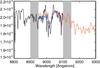 |
Fig. 1 Illustration of the combination of the MIUSCAT models (black line) with the IRTF based models (red solid line) between 8950 Å and 9100 Å. The blue line shows the combined model, obtained by means of a slight adjustment which we performed on the IRTF- based model spectra in order to end up with the same continuum flux as the extended MILES model spectra. The continuum fluxes were measured within the two narrow grey-shaded bands ranging from 8900 to 8950 Å and from 9100 to 9150 Å, respectively. Here, we plot model spectra of Solar metallicity and of an age of 10 Gyr, based on Padova00 isochrones. Note the significantly higher resolution of the MIUSCAT model spectrum compared to the IRTF-based one. |
It is remarkable that the IRTF-based model spectra had to be modified only very little to end up with the same continuum flux as the MILES-based ones. Without introducing any correction, the continuum fluxes of the two sets of model spectra already agree within an accuracy of <2% in the joining region. The reason for this is the excellent flux calibration of both the IRTF library and of the CaT library (Cenarro et al. 2001) which was used to account for the gap redwards of the wavelength range of the MILES stellar library. Conroy & van Dokkum (2012) for example carried out a similar approach of using MILES spectra in the optical and IRTF spectra in the NIR as input for their models. To bridge the gap between 7400 and 8150 Å, they made use of synthetic spectra. They, however, encountered problems with the flux calibration and as a result the colours measured from their models are only accurate to around ≈5%.
We decided to use the IRTF-based models throughout the joining region since this reddest part of the MIUSCAT models, based on the Indo-U.S. library, is characterized by a limited flux-calibration quality and strong telluric residuals (see V12). The MILES SSP models have a constant FWHM resolution of approximately 2.5 Å, while the IRTF-based ones in the IR are calculated for a constant instrumental velocity dispersion of σ = 60 km s-1. Hence, in order to correctly perform the joining, in the region between 8950 and 9100 Å, we smoothed the MILES SSP spectra to a constant FWHM of 4.2 Å, which corresponds to a velocity dispersion of σ = 60 km s-1. However,we stress that we kept the MILES part of the models at its constant FWHM resolution of ≈2.5 Å and the IRTF part at its constant spectral resolution of R ≈ 2000 after joining the models. Thus, at a wavelength of 8950 Å, there is a sudden change in resolution. The IRTF-based models were rebinned to the same pixel size of 0.9 Å pixel-1 as the MIUSCAT models.
3. Colours measured from our models
In this Section, we first check the internal consistency and correctness of our models by comparing several optical-NIR colours derived from them to the so-called photometric predictions for these colours (see Sect. 3.1). The latter ones are based on the MILES models in the optical as well as on various colour-temperature relations. Moreover, we carry out a detailed comparison with the colours predicted by other models in the literature (Sect. 3.2). Finally, we show the ability of our models to fit various optical and NIR colours observed for early-type galaxies (ETGs, see Sect. 3.3).
In order to obtain colours from our SSP model spectra, we multiply them by the transmission of the respective filters and integrate. In this procedure, we calibrate the resulting magnitudes based on the Vega-spectrum of Castelli & Kurucz (1994) as a zeropoint. We have to keep in mind that according to Ricciardelli et al. (2012) the colours of Vega are assumed to be (V − R) = 0 mag and (V − I) = − 0.04 mag in the Johnson-Cousins filters. Thus, we have to correct our obtained colours according to the latter relation.
In this work we are particularly interested in optical – NIR colours, i.e., colours combining filters from the optical and the NIR range of our joined SSP model spectra. Consequently, we calculated the magnitudes in the Buser V (Buser 1978), Cousins R and I and the Johnson J and K-bands (Bessell 1979). Since the influence of the IMF on the colours predicted by our models is almost negligible (R15), we restrict our colour analysis to SSP models based on Kroupa IMFs.
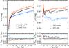 |
Fig. 2 Upper panels: comparison between the behaviour with age of the (V − R) and the (J − K) colours extracted from our model spectra (based on Padova00 isochrones) and the same colours from the MILES photometric predictions (see http://miles.iac.es; Vazdekis et al. 2010, 2015). The dotted lines delineate the MILES photometric predictions and the solid ones the colours calculated from our SSP model spectra. The different colours and symbols represent three different metallicites (see legend). Lower panels: visualization of the absolute differences between the colours measured from our model spectra and the photometrically predicted ones. |
3.1. Checking the internal consistency of the model colours
In Figs. 2–5, we compare various optical – NIR colours as calculated from our model SSPs with the same colours from the MILES photometric predictions. Since these photometric predictions have only been published based on Padova002, we present only comparisons to models using this set of isochrones. We also compared, however, the same model colours to the photometric predictions based on BaSTI isochrones and obtained very similar results. The photometric colour predictions have been determined by integrating the stellar fluxes obtained from the colour-temperature relations determined for dwarfs (Alonso et al. 1996) and for giants (Alonso et al. 1999) of spectral types F0-K5. These relations are based on extensive photometric stellar libraries and are in general metallicity dependent. Note that these colours are not obtained by integrating any synthesized SSP model SEDs within the bandpass of a filter. Since we have also used the same colour-temperature relations in order to transform the theoretical parameters (Teff, log(g), [Fe/H]) of our models to the observational plane (see Sect. 2.1), we expect a close agreement between the colours from our models and those originating from the photometric predictions.
As can be seen from the lower panels of Figs. 2–5, the differences between the colours Δ(colour) = (colour)SSP − models − (colour)phot.predictions are indeed almost for all cases smaller than the photometric precision of 0.02 mag. Slightly larger differences can usually be observed for the young ages (<2 Gyr), which is due to the lower quality of our models in this age range (see Sect. 2) caused by the limited number of AGB and carbon stars in the IRTF library. In the NIR, these types of stars contribute significantly to the total flux at these young ages (e.g. Maraston 2005; Maraston et al. 2009; Maraston & Strömbäck 2011). Apart from that, the differences between the colours measured directly from the spectra and the ones from the photometric predictions tend to be the largest in the models with supersolar metallicity, [ Fe / H ] = − 0.22. These are also of lower quality compared to their counterparts of Solar and subsolar metallicity since the coverage in parameter space is rather poor for such metallicities in the IRTF library (compare to Sect. 8.3 in R15).
The good agreement which we find between the colours measured from our model spectra and the photometrically predicted ones confirms that we have carried out correctly the modelling process and that hence our models are internally consistent. It also shows the good flux calibration of the IRTF stellar library which we confirmed in R15. Moreover, also in the optical range, Ricciardelli et al. (2012) found differences of the order of only 0.01 − 0.02 mag between the synthetic and the photometric colours. To test whether the joining of the optical with the infrared part of our models was done correctly, the colours containing the I filter are particularly interesting, since that encompasses the joining region of the models from 8900 to 9150 Å. The same holds for colours composed of an optical and a NIR band like (V − J) and (V − K). The fact that these colours do not show a worse agreement with the photometric predictions than pure optical or NIR colours proves the robustness of our method of joining the MIUSCAT spectral range with the IRTF-based one described above (see Sect. 2.2).
3.2. Comparison to other model predictions in the literature
We now compare the predictions of our models for colours to other models available in the literature which cover the optical and NIR wavelength range. These are in the first place the models by Maraston (1998, 2005), Maraston et al. (2009, hereafter Maraston models) and the ones by Conroy & van Dokkum (2012, hereafter CvD models). Furthermore, the Padova group has presented colour predictions in this wavelength range based on their library of stellar isochrones (Marigo et al. 2008). Recently Meneses-Goytia et al. (2015b) published SSP models in the NIR between 9300 and 24 100 Å which are also based on the stars of the IRTF library. In what follows, we summarize the main characteristics of all these models.
Maraston models
The Maraston models are calculated for the sets of isochrones developed by Cassisi et al. (1997), Cassisi & Salaris (1997) and Cassisi et al. (2000) and use as input the theoretical stellar spectra of the BaSeL stellar library (Lejeune et al. 1998). The spectra of the BaSeL library are based on stellar atmospheres from Kurucz (1992) and, in the case of M giants, from Fluks et al. (1994) and Bessell et al. (1989, 1991). For TP-AGB stars, Maraston (2005) include the empirical spectra of the library of Lançon & Mouhcine (2002).
Model predictions by the Padova group
Marigo et al. (2008, hereafter Marigo models) also make use of the Kurucz stellar atmospheres. More in detail, they work with the revised ATLAS9 model spectra by Castelli & Kurucz (2003), while adopting the model atmospheres of Allard et al. (2000) for M, L and T dwarfs and those of Fluks et al. (1994) for M giants. Contrary to the Maraston models, the Marigo models employ the synthetic spectra of Loidl et al. (2001) for TP-AGB stars. The main caveat of the Marigo models is that they give only colour predictions and do not provide model spectra.
CvD models
Conroy & van Dokkum (2012), however, followed an approach comparable to ours by combining stellar spectra of the two empirical stellar libraries MILES (Sánchez-Blázquez et al. 2006) and IRTF (Rayner et al. 2009) with similar parameters. The MILES spectra cover the spectral range between 0.35 and 0.74 μm, whereas the IRTF stars are available for wavelengths between 0.81 and 2.4 μm. In order to fill in the gap between the two stellar libraries and also in order to incorporate the possibility to change individual element abundances, Conroy & van Dokkum (2012) used the ATLAS model atmospheres (Kurucz 1992). It should be noticed that Conroy & van Dokkum (2012) used a subsample of the IRTF library only about half the size of ours (91 stars) by placing quite strong constraints on the individual stars (only luminosity classes III or V, measured parallaxes available). Moreover, as mentioned in Sect. 2.2, colours measured from their models are less accurate than colours obtained from our models. To reproduce the main sequence and red giant branch evolutionary phases, Conroy & van Dokkum (2012) applied the Dartmouth isochrones (Dotter et al. 2008). This set of isochrones, however, does not exist for evolutionary phases beyond the core helium ignition. Hence, they used the Padova isochrones (Marigo et al. 2008) for the horizontal and asymptotic branches.
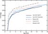 |
Fig. 6 Comparison of the behaviour of the (V − R) colour as a function of age for three different models (see legend) and our own (BaSTI- and Padova00-based) ones. All the displayed models are of solar metallicity and based on an underlying Kroupa IMF. |
Discussion
Figure 6 shows the predicted (V − R) colours extracted from both our Padova00- and BaSTI-based SSP models, as well as from the three sets of models discussed above (see legend). We see that in (V − R), all of the models from the literature follow the same trend as our SSP models and become redder with increasing age. The largest change in colour can be observed for ages between 1 and 3 Gyr, while the reddening is less abrupt for older ages. For the youngest ages, the Marigo models trace best the predictions from our SSP models. However, they exhibit the largest difference (Δ ≈ 0.03 − 0.05) for ages older than 3 Gyr. In this age interval, the Maraston models and the Conroy ones agree closest with our models. Moreover, for these older ages, the predictions of our models show a good agreement with the observed colours of globular clusters, as can be seen from Figs. 1 and 3 in Ricciardelli et al. (2012).
As Fig. 7 shows, the difference between the sets of models is much more pronounced for (J − K). Both of our SSP models show a moderate peak towards red colours for ages between 1 and 2 Gyr, before becoming slightly redder again for older ages. We attribute this peak to the AGB and TP-AGB stars which are the main contributors to the integrated IR light at these intermediate ages. The same peak – though considerably stronger – becomes visible in the Marigo models. For ages larger than 3 Gyr, this set of models gives gradually slightly bluer colours. This behaviour, which is contrary to what we observe in our models, is also observed in the (J − K) colours of the CvD models. However, while the Marigo models coincide very well with ours for ages older than 3 Gyr, the CvD models are too blue by about Δ(J − K) ≈ 0.06 for ages larger than 7 Gyr. Due to an enhanced AGB star contribution (see also Maraston 1998, 2005; Maraston et al. 2009), the Maraston models show the reddest colours between 1 and 2 Gyr of all the models considered here. At ages of 1 Gyr, the peak has apparently not yet been reached, and the reddening seems to continue for younger ages. Then, the (J − K) colour decreases rapidly until reaching a minimum at around 3 Gyr. For older ages, the (J − K) colour becomes redder again, while always staying too blue by at least Δ(J − K) ≈ 0.07 with respect to the predicted colours of our models.
Recently, Zibetti et al. (2013) has risen serious doubts about the much enhanced contribution of TP-AGB stars to the Maraston-models which results in the red colours for ages between 1 and 3 Gyr in Fig. 7. Zibetti et al. (2013) were unable to reproduce the observed optical-NIR colours of their 16 post-starburst galaxies with any combination of stellar populations based on the Maraston models. Despite the somewhat bluer colours predicted for older ages, both the assumption of a simple stellar population or a scenario of a recent burst of star formation together with an underlying old population yielded colours which were too red compared to their observations.
The comparison carried out here for the (J − K) colour with our models and those of Marigo and CvD highlights the overly extreme behaviour of the Maraston models. In order to compensate the very red colours at younger ages caused by the large fraction of AGB stars contributing to their models, they end up with too blue colours at older ages.
Models by Meneses-Goytia et al. (2015b)
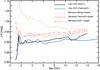 |
Fig. 8 As Fig. 7, but comparing the (J − K) colours of the three different sets of Meneses-models to our own (BaSTI- and Padova00-based) ones. |
To construct their models (hereafter Meneses-models), Meneses-Goytia et al. (2015b) excluded less stars from the IRTF library than we did and they also determined their atmospheric parameters differently. While we used both colour-temperature relations and a large literature compilation (Röck et al. 2015), Meneses-Goytia et al. (2015a) determined the stellar atmospheric parameters using full-spectrum fitting based on ULySS (Koleva et al. 2009). Moreover, they slightly changed the interpolator code (Vazdekis et al. 2003)3. In addition to the BaSTI and the Padova00 isochrones, Meneses-Goytia et al. (2015b) computed their models also based on the set of isochrones by Marigo et al. (2008).
Figure 8 shows a comparison between our model predictions for the (J − K) colour and those of the different sets of Meneses-models. The colours originating from our models based on the BaSTI and the Padova00 isochrones agree well with those of the corresponding sets of the Meneses-models. Compared to our models, the latter ones are, however, generally redder by Δ(J − K) = 0.03 mag. This difference can be explained by the different adopted atmospheric parameters with respect to our models, in particular for the coolest stars. In addition, our models offer the advantage of a much larger wavelength coverage, since they include the whole optical wavelength range and extend up to 5 μm.
The set of Meneses-models calculated using the isochrones of Marigo et al. (2008) show a very similar overall behaviour to the colour predictions of the Marigo models (see Fig. 7). The former yield, however, colours which are redder by about Δ(J − K) = 0.07 − 0.08 mag and their increase due to the contribution of AGB stars at ages smaller than 2 Gyr is even more pronounced than in the Marigo models. Contrary to, e.g. the Maraston-models, the (J − K) colours originating from this set of Meneses-models also do not decrease significantly towards bluer colours for older ages. Moreover, the NIR-colours of the observed ETGs can be only fitted by models of low metallicities of [ Fe / H ] = −0.4–−0.7 (see Fig. 10 in Meneses-Goytia et al. 2015b). However, stellar population analysis in the optical range renders such low metallicities for ETGs extremely unlikely.
3.3. Reproducing observed colours of ETGs
Figure 9 shows the optical colour (B − V) as a function of the NIR colour (J − K) for a selected sample of ETGs together with the predictions from our models. The 2MASS (J − K) colours were taken from the 2MASS Large Galaxy Atlas (Jarrett et al. 2003) while the corresponding optical (B − V) colours come from the HyperLeda4 database (Makarov et al. 2014). The colours of our models fit very well those of the observed galaxies. This proves that our combined models qualify perfectly to reproduce all the colours from the optical until the MIR range.
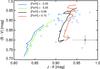 |
Fig. 9 (B − V) versus (J − K) diagram showing our models overplotted on a sample of ETGs (blue diamonds). The uncertainties in both colours are indicated by an error bar. We display the predictions of our models based on BaSTI isochrones for ages between 1 and 14 Gyr and various metallicities (see legend). |
In Fig. 10, we compare the colour predictions of our models in the NIR to the observed colours of the central regions of 51 bright ETGs (mostly ellipticals and S0) at small redshifts (z< 0.022) observed by Frogel et al. (1978). All of their colours are corrected to the restframe. Additionally, we also overplot the colour predictions of the Maraston and the CvD models for Solar metallicities, Kroupa-like IMFs and ages older than 1 Gyr and 3 Gyr, respectively. For both examined colours, (J − K) and (J − H), our models provide good fits. Like in the optical range, the observed colours can be reproduced well by an old, single stellar population without the need for an additional young component. Our models coincide with the mean colours of the observed sample in both colours. At the same time, the models also trace a substantial part of the scatter in the colours. Both colours are hampered by the age-metallicity degeneracy, i.e. they become redder with both increasing age and metallicity. Consequently, the bluer galaxies can be both more metal-poor and younger than their redder counterparts.
Both the colours obtained from the CvD models and from the Maraston ones show a worse agreement with the observations than the colours originating from our SSP models. While the CvD models yield somewhat too blue (J − K) colours compared to the bulk of ETGs, the Maraston models fit the observations reasonably well only for the very youngest ages between 1 and 2 Gyr. For ages older than 2 Gyr, the Maraston models provide colours which are all too blue with respect to the observed ETGs of Frogel et al. (1978). We noted this very extreme behaviour of the Maraston models already in Fig. 7 in Sect. 3.2. Contrary to the Maraston models, our models allow us to fit the colours of the observed galaxies with a single SSP without the need for a contribution of an additional young population, which is in good agreement with detailed studies in the optical range.
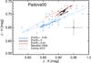 |
Fig. 10 (J − H) versus (J − K) diagram of the ETGs of Frogel et al. (1978; blue diamonds). Overplotted are the corresponding colours predicted from our SSP models based on Padova00 isochrones (solid lines, colours indicate different metallicities according to the legend) as well as those originating from the Maraston models (blue dotted line) and from the CvD models (red dashed line). Both of these sets of models were computed for Solar metallicity and for ages larger than 1 Gyr (Maraston models) and 3 Gyr (CvD models), respectively. The observed uncertainties in both colours are indicated by an error bar. |
4. Summary
We present the first evolutionary stellar population models covering the wavelength range from 3465 to 50 000 Å which are – apart from two gaps which were covered with the help of theoretical libraries – based on empirical stellar spectra. We obtained this large wavelength coverage by combining the extended MILES models (V10; V12) in the optical range with the models based on the IRTF library (Cushing et al. 2005; Rayner et al. 2009) in the NIR and MIR between 8150 and 50 000 Å (R15).
The actual matching was carried out between 8950 and 9100 Å (see Sect. 2.2). Thanks to the excellent flux calibration of the stellar spectra of both the MILES and the IRTF library, we had to adjust only slightly the fluxes in the joining region. Nevertheless, due to this slight artificial modification of the flux one should refrain from measuring line strength indices in this matching region. However, it is completely safe to obtain all kinds of optical and NIR/MIR colours by integrating the model spectra over the respective filter bandpasses. When determining line strength indices from our combined SSP models, one should be aware that the MILES-based part of the models is kept at the FWHM resolution of 2.5 Å, while the IRTF-based part redwards of 8950 Å is given at the constant spectral resolution of R ≈ 2000.
We calculated our models based on both BaSTI (Pietrinferni et al. 2004) and Padova00 (Girardi et al. 2000) isochrones. Our models are available for a large range of underlying IMFs, like Kroupa, revised Kroupa and unimodal and bimodal of slopes varying between Γ = 0.3 and 3.3.
We conclude that our SSP models are internally consistent due to the close agreement of optical and NIR colours obtained from them with the colours originating from the predictions based on extensive photometric libraries published on our web page2. Even colours composed of filters encompassing the joining region between our two sets of models usually do not deviate more than the photometric limit of 0.02 mag from the ones obtained from the photometric predictions.
We also compared the predictions of our SSP models to those of other models which are available in the literature for the optical and NIR wavelength range. The observed differences between the theoretical Maraston, Marigo and the semiempirical CvD models and our two sets of Padova00 and BaSTI based SSP models are rather small in the case of the pure optical (V − R) colour. For a NIR colour like (J − K), some differences between the various sets of models arise from the different treatment of the TP-AGB evolutionary phase. Compared to our newly combined SSP models, the models of Marigo and in particular those of Maraston show a much more pronounced contribution of AGB stars which gets reflected in significantly redder colours with respect to our models for ages younger than 2 Gyr. For ages older than 3 Gyr, our SSP models agree best with the Marigo models, while the Maraston models show bluer colours compared to our models. The Meneses-models which are based on a comparable sample of stars from the IRTF library yield slightly redder colours in the case of underlying BaSTI andPadova00 isochrones. Their set of models calculated using the isochrones by Marigo et al. (2008), however, results in too red colours over the whole age range with respect to our models and in too low metallicities for the ETGs compared to what we know from the optical range. Moreover, our models offer the additional advantage of a much larger wavelength coverage.
Different optical and NIR colours measured from our SSP models are in good agreement with the observed colours from ETGs. Like in the optical spectral range, we are able to fit these galaxies with just one, old single-burst like stellar population and we do not need to assume an additional young component as is the case for other models in the literature.
Our combined models are available on the MILES webpage2. Future work will focus on achieving a better understanding of the poorly analyzed absorption line features in the NIR from both a modeling and observational point of view.
Acknowledgments
We acknowledge financial support to the DAGAL network from the People Programme (Marie Curie Actions) of the European Union’s Seventh Framework Programme FP7/2007–2013/ under REA grant agreement number PITN-GA-2011-289313, and from the Spanish Ministry of Economy and Competitiveness (MINECO) under grant numbers AYA2013-41243-P and AYA2013-Y8226-C3-1-P. J.H.K. thanks the Astrophysics Research Institute of Liverpool John Moores University for their hospitality, and the Spanish Ministry of Education, Culture and Sports for financial support of his visit there, through grant number PR2015-00512.
References
- Allard, F., Hauschildt, P. H., Alexander, D. R., Ferguson, J. W., & Tamanai, A. 2000, in From Giant Planets to Cool Stars, eds. C. A. Griffith, & M. S. Marley, ASP Conf. Ser., 212, 127 [Google Scholar]
- Allard, F., Homeier, D., & Freytag, B. 2012, Roy. Soc. Lond. Philosoph. Trans. Ser. A, 370, 2765 [Google Scholar]
- Alonso, A., Arribas, S., & Martinez-Roger, C. 1996, A&A, 313, 873 [NASA ADS] [Google Scholar]
- Alonso, A., Arribas, S., & Martínez-Roger, C. 1999, A&AS, 140, 261 [NASA ADS] [CrossRef] [EDP Sciences] [Google Scholar]
- Bessell, M. S. 1979, PASP, 91, 589 [NASA ADS] [CrossRef] [Google Scholar]
- Bessell, M. S., Brett, J. M., Wood, P. R., & Scholz, M. 1989, A&AS, 77, 1 [NASA ADS] [Google Scholar]
- Bessell, M. S., Brett, J. M., Scholz, M., & Wood, P. R. 1991, A&AS, 89, 335 [NASA ADS] [Google Scholar]
- Bruzual, G., & Charlot, S. 2003, MNRAS, 344, 1000 [NASA ADS] [CrossRef] [Google Scholar]
- Buser, R. 1978, A&A, 62, 411 [NASA ADS] [Google Scholar]
- Cassisi, S., & Salaris, M. 1997, MNRAS, 285, 593 [NASA ADS] [Google Scholar]
- Cassisi, S., Castellani, M., & Castellani, V. 1997, A&A, 317, 108 [NASA ADS] [Google Scholar]
- Cassisi, S., Castellani, V., Ciarcelluti, P., Piotto, G., & Zoccali, M. 2000, MNRAS, 315, 679 [NASA ADS] [CrossRef] [Google Scholar]
- Castelli, F., & Kurucz, R. L. 1994, A&A, 281, 817 [NASA ADS] [Google Scholar]
- Castelli, F., & Kurucz, R. L. 2003, in Modelling of Stellar Atmospheres, eds. N. Piskunov, W. W. Weiss, & D. F. Gray, IAU Symp., 210, 20 [Google Scholar]
- Cenarro, A. J., Gorgas, J., Cardiel, N., et al. 2001, MNRAS, 326, 981 [NASA ADS] [CrossRef] [Google Scholar]
- Cenarro, A. J., Peletier, R. F., Sánchez-Blázquez, P., et al. 2007, MNRAS, 374, 664 [NASA ADS] [CrossRef] [Google Scholar]
- Chen, Y.-P., Trager, S. C., Peletier, R. F., et al. 2014, A&A, 565, A117 [NASA ADS] [CrossRef] [EDP Sciences] [Google Scholar]
- Conroy, C., & van Dokkum, P. 2012, ApJ, 747, 69 [NASA ADS] [CrossRef] [Google Scholar]
- Conroy, C., Gunn, J. E., & White, M. 2009, ApJ, 699, 486 [NASA ADS] [CrossRef] [Google Scholar]
- Cushing, M. C., Rayner, J. T., & Vacca, W. D. 2005, ApJ, 623, 1115 [NASA ADS] [CrossRef] [Google Scholar]
- Dotter, A., Chaboyer, B., Jevremović, D., et al. 2008, ApJS, 178, 89 [NASA ADS] [CrossRef] [Google Scholar]
- Fluks, M. A., Plez, B., The, P. S., et al. 1994, A&AS, 105, 311 [NASA ADS] [Google Scholar]
- Frogel, J. A., Persson, S. E., Matthews, K., & Aaronson, M. 1978, ApJ, 220, 75 [NASA ADS] [CrossRef] [Google Scholar]
- Girardi, L., Bressan, A., Bertelli, G., & Chiosi, C. 2000, A&AS, 141, 371 [NASA ADS] [CrossRef] [EDP Sciences] [Google Scholar]
- Husser, T.-O., Wende-von Berg, S., Dreizler, S., et al. 2013, A&A, 553, A6 [NASA ADS] [CrossRef] [EDP Sciences] [Google Scholar]
- Jarrett, T. H., Chester, T., Cutri, R., Schneider, S. E., & Huchra, J. P. 2003, AJ, 125, 525 [NASA ADS] [CrossRef] [Google Scholar]
- Koleva, M., Prugniel, P., Bouchard, A., & Wu, Y. 2009, A&A, 501, 1269 [NASA ADS] [CrossRef] [EDP Sciences] [Google Scholar]
- Kroupa, P. 2001, MNRAS, 322, 231 [NASA ADS] [CrossRef] [Google Scholar]
- Kurucz, R. L. 1992, in The Stellar Populations of Galaxies, eds. B. Barbuy, & A. Renzini, IAU Symp., 149, 225 [Google Scholar]
- Lançon, A., & Mouhcine, M. 2002, A&A, 393, 167 [NASA ADS] [CrossRef] [EDP Sciences] [Google Scholar]
- Lançon, A., & Wood, P. R. 2000, A&AS, 146, 217 [NASA ADS] [CrossRef] [EDP Sciences] [Google Scholar]
- Le Borgne, J.-F., Bruzual, G., Pelló, R., et al. 2003, A&A, 402, 433 [NASA ADS] [CrossRef] [EDP Sciences] [Google Scholar]
- Le Borgne, D., Rocca-Volmerange, B., Prugniel, P., et al. 2004, A&A, 425, 881 [NASA ADS] [CrossRef] [EDP Sciences] [Google Scholar]
- Lejeune, T., Cuisinier, F., & Buser, R. 1997, A&AS, 125, 229 [NASA ADS] [CrossRef] [EDP Sciences] [Google Scholar]
- Lejeune, T., Cuisinier, F., & Buser, R. 1998, A&AS, 130, 65 [NASA ADS] [CrossRef] [EDP Sciences] [Google Scholar]
- Loidl, R., Lançon, A., & Jørgensen, U. G. 2001, A&A, 371, 1065 [NASA ADS] [CrossRef] [EDP Sciences] [Google Scholar]
- Makarov, D., Prugniel, P., Terekhova, N., Courtois, H., & Vauglin, I. 2014, A&A, 570, A13 [Google Scholar]
- Maraston, C. 1998, MNRAS, 300, 872 [NASA ADS] [CrossRef] [Google Scholar]
- Maraston, C. 2005, MNRAS, 362, 799 [NASA ADS] [CrossRef] [Google Scholar]
- Maraston, C., & Strömbäck, G. 2011, MNRAS, 418, 2785 [NASA ADS] [CrossRef] [Google Scholar]
- Maraston, C., Strömbäck, G., Thomas, D., Wake, D. A., & Nichol, R. C. 2009, MNRAS, 394, L107 [NASA ADS] [CrossRef] [Google Scholar]
- Marigo, P., Girardi, L., Bressan, A., et al. 2008, A&A, 482, 883 [NASA ADS] [CrossRef] [EDP Sciences] [Google Scholar]
- Meneses-Goytia, S., Peletier, R. F., Trager, S. C., et al. 2015a, A&A, 582, A96 [NASA ADS] [CrossRef] [EDP Sciences] [Google Scholar]
- Meneses-Goytia, S., Peletier, R. F., Trager, S. C., & Vazdekis, A. 2015b, A&A, 582, A97 [NASA ADS] [CrossRef] [EDP Sciences] [Google Scholar]
- Pickles, A. J. 1998, PASP, 110, 863 [CrossRef] [Google Scholar]
- Pietrinferni, A., Cassisi, S., Salaris, M., & Castelli, F. 2004, ApJ, 612, 168 [NASA ADS] [CrossRef] [Google Scholar]
- Prugniel, P., & Soubiran, C. 2001, A&A, 369, 1048 [NASA ADS] [CrossRef] [EDP Sciences] [Google Scholar]
- Rayner, J. T., Cushing, M. C., & Vacca, W. D. 2009, ApJS, 185, 289 [NASA ADS] [CrossRef] [Google Scholar]
- Ricciardelli, E., Vazdekis, A., Cenarro, A. J., & Falcón-Barroso, J. 2012, MNRAS, 424, 172 [NASA ADS] [CrossRef] [Google Scholar]
- Röck, B., Vazdekis, A., Peletier, R. F., Knapen, J. H., & Falcón-Barroso, J. 2015, MNRAS, 449, 2853 [NASA ADS] [CrossRef] [Google Scholar]
- Sánchez-Blázquez, P., Peletier, R. F., Jiménez-Vicente, J., et al. 2006, MNRAS, 371, 703 [NASA ADS] [CrossRef] [Google Scholar]
- Valdes, F., Gupta, R., Rose, J. A., Singh, H. P., & Bell, D. J. 2004, ApJS, 152, 251 [NASA ADS] [CrossRef] [Google Scholar]
- Vazdekis, A. 1999, ApJ, 513, 224 [NASA ADS] [CrossRef] [Google Scholar]
- Vazdekis, A., Casuso, E., Peletier, R. F., & Beckman, J. E. 1996, ApJS, 106, 307 [NASA ADS] [CrossRef] [Google Scholar]
- Vazdekis, A., Cenarro, A. J., Gorgas, J., Cardiel, N., & Peletier, R. F. 2003, MNRAS, 340, 1317 [NASA ADS] [CrossRef] [Google Scholar]
- Vazdekis, A., Sánchez-Blázquez, P., Falcón-Barroso, J., et al. 2010, MNRAS, 404, 1639 [NASA ADS] [Google Scholar]
- Vazdekis, A., Ricciardelli, E., Cenarro, A. J., Rivero-González, J. G., & Díaz-García, L. A. 2012, MNRAS, 424, 157 [NASA ADS] [CrossRef] [Google Scholar]
- Vazdekis, A., Coelho, P., Cassisi, S., et al. 2015, MNRAS, 449, 1177 [NASA ADS] [CrossRef] [Google Scholar]
- Westera, P., Lejeune, T., Buser, R., Cuisinier, F., & Bruzual, G. 2002, A&A, 381, 524 [NASA ADS] [CrossRef] [EDP Sciences] [Google Scholar]
- Worthey, G. 1994, ApJS, 95, 107 [NASA ADS] [CrossRef] [Google Scholar]
- Zibetti, S., Gallazzi, A., Charlot, S., Pierini, D., & Pasquali, A. 2013, MNRAS, 428, 1479 [NASA ADS] [CrossRef] [Google Scholar]
All Tables
All Figures
|
Fig. 1 Illustration of the combination of the MIUSCAT models (black line) with the IRTF based models (red solid line) between 8950 Å and 9100 Å. The blue line shows the combined model, obtained by means of a slight adjustment which we performed on the IRTF- based model spectra in order to end up with the same continuum flux as the extended MILES model spectra. The continuum fluxes were measured within the two narrow grey-shaded bands ranging from 8900 to 8950 Å and from 9100 to 9150 Å, respectively. Here, we plot model spectra of Solar metallicity and of an age of 10 Gyr, based on Padova00 isochrones. Note the significantly higher resolution of the MIUSCAT model spectrum compared to the IRTF-based one. |
| In the text | |
|
Fig. 2 Upper panels: comparison between the behaviour with age of the (V − R) and the (J − K) colours extracted from our model spectra (based on Padova00 isochrones) and the same colours from the MILES photometric predictions (see http://miles.iac.es; Vazdekis et al. 2010, 2015). The dotted lines delineate the MILES photometric predictions and the solid ones the colours calculated from our SSP model spectra. The different colours and symbols represent three different metallicites (see legend). Lower panels: visualization of the absolute differences between the colours measured from our model spectra and the photometrically predicted ones. |
| In the text | |
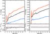 |
Fig. 3 Same as Fig. 2, but for (V − J) and (V − K) colours. |
| In the text | |
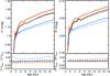 |
Fig. 4 Same as Fig. 2, but for (V − I) and (R − I) colours. |
| In the text | |
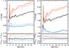 |
Fig. 5 Same as Fig.2, but for (I − J) and (I − K) colours. |
| In the text | |
|
Fig. 6 Comparison of the behaviour of the (V − R) colour as a function of age for three different models (see legend) and our own (BaSTI- and Padova00-based) ones. All the displayed models are of solar metallicity and based on an underlying Kroupa IMF. |
| In the text | |
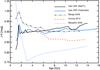 |
Fig. 7 Same as Fig. 6, but for the (J − K) colour. |
| In the text | |
|
Fig. 8 As Fig. 7, but comparing the (J − K) colours of the three different sets of Meneses-models to our own (BaSTI- and Padova00-based) ones. |
| In the text | |
|
Fig. 9 (B − V) versus (J − K) diagram showing our models overplotted on a sample of ETGs (blue diamonds). The uncertainties in both colours are indicated by an error bar. We display the predictions of our models based on BaSTI isochrones for ages between 1 and 14 Gyr and various metallicities (see legend). |
| In the text | |
|
Fig. 10 (J − H) versus (J − K) diagram of the ETGs of Frogel et al. (1978; blue diamonds). Overplotted are the corresponding colours predicted from our SSP models based on Padova00 isochrones (solid lines, colours indicate different metallicities according to the legend) as well as those originating from the Maraston models (blue dotted line) and from the CvD models (red dashed line). Both of these sets of models were computed for Solar metallicity and for ages larger than 1 Gyr (Maraston models) and 3 Gyr (CvD models), respectively. The observed uncertainties in both colours are indicated by an error bar. |
| In the text | |
Current usage metrics show cumulative count of Article Views (full-text article views including HTML views, PDF and ePub downloads, according to the available data) and Abstracts Views on Vision4Press platform.
Data correspond to usage on the plateform after 2015. The current usage metrics is available 48-96 hours after online publication and is updated daily on week days.
Initial download of the metrics may take a while.