| Issue |
A&A
Volume 589, May 2016
|
|
|---|---|---|
| Article Number | A42 | |
| Number of page(s) | 12 | |
| Section | Astrophysical processes | |
| DOI | https://doi.org/10.1051/0004-6361/201527501 | |
| Published online | 12 April 2016 | |
IGR J17451–3022: A dipping and eclipsing low mass X-ray binary
1
ISDC Data Centre for Astrophysics, Chemin d’Ecogia 16, 1290
Versoix,
Switzerland
e-mail: This email address is being protected from spambots. You need JavaScript enabled to view it.
2
Centrum Astronomiczne im. M. Kopernika,
Bartycka 18, 00-716
Warszawa,
Poland
3
Department of Astrophysical Sciences, Princeton
University, 4 Ivy
Lane, NJ
08544
Princeton,
USA
4
INAF, Istituto di Astrofisica Spaziale e Fisica Cosmica –
Palermo, via U. La Malfa
153, 90146
Palermo,
Italy
5
Institut de Ciències de l’Espai (IEEC-CSIC),
Campus UAB, carrer de Can Magrans, S/N 08193,
Cerdanyola del Vallès, Barcelona, Spain
6
Astrohpysics, Department of Physics, University of
Oxford, Keble Road,
Oxford
OX1 3RH,
UK
7
Universitá degli Studi di Cagliari, Dipartimento di
Fisica, SP Monserrato-Sestu, KM
0.7, 09042
Monserrato,
Italy
8
INAF-Istituto di Astrofisica Spaziale e Fisica Cosmica –
Milano, via E. Bassini
15, 20133
Milano,
Italy
9
Dipartimento di Fisica e Chimica, Universitá di
Palermo, via Archirafi
36, 90123
Palermo,
Italy
10
Department of Physics, Oregon State University,
301 Weniger Hall, Corvallis, OR
97331,
USA
11
Max-Planck-Institut für Extraterretrische Physik,
Giessenbachstrasse,
85748
Garching,
Germany
Received:
4
October
2015
Accepted:
7
March
2016
Abstract
In this paper we report on the available X-ray data collected by INTEGRAL, Swift, and XMM-Newton during the first outburst of the INTEGRAL transient IGR J17451–3022, discovered in 2014 August. The monitoring observations provided by the JEM-X instruments on board INTEGRAL and the Swift /XRT showed that the event lasted for about 9 months and that the emission of the source remained soft for the entire period. The source emission is dominated by a thermal component (kT ~ 1.2 keV), most likely produced by an accretion disk. The XMM-Newton observation carried out during the outburst revealed the presence of multiple absorption features in the soft X-ray emission that could be associated with the presence of an ionized absorber lying above the accretion disk, as observed in many high inclination, low mass X-ray binaries. The XMM-Newton data also revealed the presence of partial and rectangular X-ray eclipses (lasting about 820 s) together with dips. The rectangular eclipses can be associated with increases in the overall absorption column density in the direction of the source. The detection of two consecutive X-ray eclipses in the XMM-Newton data allowed us to estimate the source orbital period at Porb = 22620.5+2.0-1.8 s (1σ confidence level).
Key words: X-rays: individuals: IGR J17451-3022 / X-rays: binaries
© ESO, 2016
1. Introduction
IGR J17451–3022 is an X-ray transient discovered by INTEGRAL on 2014 August 22 during the observations performed in the direction of the Galactic center (Chenevez et al. 2014). The source underwent a 9-month outburst and began its return to quiescence in the second half of May 2015 (Bahramian et al. 2015a). At discovery, the source displayed a relatively soft emission, significantly detected by the JEM-X instrument on board INTEGRAL only below 10 keV (Chenevez et al. 2014). The estimated 3–10 keV flux was ~7 mCrab, corresponding to roughly 10-10 erg cm-2 s-1. The outburst of IGR J17451–3022 was followed up with Swift (Altamirano et al. 2014; Heinke et al. 2014; Bahramian et al. 2015b, 2014a,b), Suzaku (Jaisawal et al. 2015), and Chandra (Chakrabarty et al. 2014). The best determined source position was obtained from the Chandra data at RA(J2000) =  , Dec(J
 , with an associated uncertainty of 0.̋6 (90% confidence level). The spectral energy distribution of the source, together with the discovery of X-ray eclipses spaced by ~6.3 h, led to the classification of this source as a low mass X-ray binary (LMXB; Bahramian et al. 2014b; Jaisawal et al. 2015).
In this paper we report on the analysis of all available Swift and INTEGRAL data collected during the outburst of the source, together with a XMM-Newton Target of Opportunity observation (ToO) that was performed on 2014 March 6 for 40 ks.
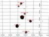 |
Fig. 1 INTEGRAL JEM-X mosaicked image around the position of IGR J17451–3022 (3–10 keV). This was obtained by using the data collected during the satellite revolutions 1448–1533 (excluding 1458; see text for details). The source is detected in this mosaic with a significance of 23.7σ. |
2. INTEGRAL data
During its outburst, IGR J17451–3022 was visible within the field of view of the two JEM-X units on board INTEGRAL from satellite revolution 1448 (starting on 2014 August 18) to 1470 (hereafter first part of the outburst) and from 1508 to 1533 (ending on 2015 April 25; hereafter second part of the outburst). We analyzed all the publicly available INTEGRAL data and those for which our group obtained access rights in the INTEGRAL AO11 by using version 10.1 of the Off-line Scientific Analysis software (OSA) distributed by the ISDC (Courvoisier et al. 2003). INTEGRAL observations are divided into “science windows” (SCWs), i.e., pointings with typical durations of ~2–3 ks. Only SCWs in which the source was located to within an off-axis angle of 4.5 deg from the center of the JEM-X field of view (Lund et al. 2003) were included in the JEM-X analysis, while for IBIS/ISGRI we retained all SCWs where the source was within an off-axis angle of 12 deg from the center of the instrument field of view. We extracted the IBIS/ISGRI (Ubertini et al. 2003; Lebrun et al. 2003) mosaics in the 20–40 keV and 40–80 keV energy bands, while the JEM-X mosaics were extracted in the 3–10 keV and 10–20 keV energy bands. We used below values from JEM-X1 as a reference to provide all quantitative results, but checked that compatible values, to within the uncertainties, would be obtained with JEM-X2.
By checking the IBIS/ISGRI mosaics of each revolution, we noticed that the source was never significantly detected except for revolution 1458, which covers the period 2014 September 21 at 19:02 UTC to September 24 at 03:24 UTC (total exposure time 158 ks). In this revolution, we estimated from the IBIS/ISGRI mosaics a source detection significance of 8.4σ in the 20–40 keV energy band and 7.8σ in the 40–80 keV energy band. The corresponding source count-rate in the two energy bands was 0.80 ± 0.10 cts s-1 and 0.54 ± 0.07 cts s-1, which translate into fluxes of 5.7 ± 0.7 mCrab (~4.4 × 10⁻¹¹ erg cm-2 s-1) and 7.2 ± 0.9 mCrab (~5.0 × 10⁻¹¹ erg cm-2 s-1), respectively1. In the IBIS/ISGRI mosaic obtained during the first part of the outburst (revolutions 1448–1470, but excluding revolution 1458), the source was only marginally detected at ~5.6σ in the 20–40 keV energy range and ~7.0σ in the 40–80 keV energy range. The count-rate of the source was roughly 0.2 cts s-1 in both energy bands, corresponding to a flux of ~1.5 mCrab in the 20–40 keV energy band and ~2.5 mCrab in the 40–80 keV energy band (i.e., ~1.2 × 10⁻¹¹ erg cm-2 s-1 and ~1.7 × 10⁻¹¹ erg cm-2 s-1, respectively). Given the relatively long cumulated exposure time of the mosaic (1.4 Ms), several structures were detected at significances close to or higher than that of IGR J17451–3022. For this reason, we cannot determine whether the fluxes measured from the position of the source are genuine or are simply due to background fluctuations arising in the crowded and complex region of the Galactic Center. We can certainly conclude that the overall flux of the source during the first part of the outburst in the IBIS/ISGRI energy band was significantly lower than that measured during the revolution 1458 alone. A similar conclusion applies to the IBIS/ISGRI mosaic extracted during the second part of the outburst, i.e., including data from revolution 1508 to 1533 (total exposure time 1.3 Ms). In this case the detection significance of the source was only 5.0σ in the 20–40 keV energy band and 3.6σ in the 40–80 keV energy range. These low significance detections are likely due to background fluctuations. We estimated in this case a 3σ upper limit on the source flux of about 2 mCrab in both the 20–40 keV and 40–80 keV energy bands (corresponding to ~1.5 × 10⁻¹¹ erg cm-2 s-1 and ~1.4 × 10⁻¹¹ erg cm-2 s-1, respectively). By combining the ISGRI data from revolutions 1448–1533, but excluding revolution 1458, we did not notice an increase in the source detection significance. In this deeper mosaic (total exposure time 2.7 Ms), the source detection was at 6σ in the 20–40 keV energy band and 7.6σ in the 40–80 keV energy band. This finding supports the idea that the mentioned low level detections in all revolutions but 1458 are likely to result from background fluctuations.
In revolution 1458, the source was detected at 5.8σ in the 3–10 keV JEM-X energy band with a count-rate of 0.80 ± 0.14 cts s-1 (total exposure time 37 ks). The estimated flux was 7.2 ± 1.2 mCrab (~1.0 × 10⁻¹⁰ erg cm-2 s-1). The source was only marginally detected (~3σ) in the 10–20 keV energy band with a count-rate of 0.17 ± 0.06 cts s-1 and a flux of 5 ± 2 mCrab (corresponding to ~4.6 × 10⁻¹¹ erg cm-2 s-1).
We did not detect significant variability of the 3–10 keV source flux in the JEM-X data collected in all other revolutions, but the corresponding flux in the 10–20 keV energy band seemed to decrease by a factor of at least ≳3. In the JEM-X mosaic built by using data from revolution 1448 to 1470 (excluding revolution 1458), the source was detected with a count-rate of 0.67 ± 0.04 cts s-1 (detection significance 16σ) in the 3–10 keV energy band and we estimated a 3σ upper limit of 2 mCrab for the flux in the 10–20 keV energy band (total exposure time 367 ks). In revolutions 1508 to 1533, the source was detected with a count-rate of 0.70 ± 0.04 cts s-1 in the 3–10 keV energy band (detection significance 18σ) and we estimated a 3σ upper limit of 2 mCrab for the flux in the 10–20 keV energy band (total exposure time 372 ks). When data from all revolutions but 1458 are merged (see Fig. 1), the estimated source count-rate in the 3–10 keV energy range is 0.68 ± 0.03 cts s-1 (detection significance 23.7σ) and the 3σ upper limit for the flux in the 10–20 keV energy band is 1 mCrab (total exposure time 738 ks).
Given the above results, we focused on the JEM-X and ISGRI spectra extracted from the data collected during satellite revolution 1458. As the source was relatively faint and the surrounding region crowded, the JEM-X spectra were extracted with the mosaic_spec tool from a mosaic with eight energy bins (spanning the range 3–25 keV) in order to avoid contamination from nearby sources. ISGRI spectra were extracted by using a response matrix with six energy bins in the range 20–100 keV. During the fit to these spectra we ignored the energy range 20–25 keV in JEM-X owing to the lack of signal from the source and the first bin in ISGRI to avoid calibration uncertainties. The combined JEM-X+ISGRI spectrum could be well fit ( /d.o.f. = 0.4/7) by using a simple absorption power-law model (the absorption column density was fixed to the best value determined from the XMM-Newton data, i.e., NH = 5.6 × 1022 cm-2; see Sect. 4). The best fit power-law photon index was Γ = 2.0 ± 0.4 and the measured absorbed flux in the 3–20 keV (20–100 keV) was 1.0 × 10⁻¹⁰ erg cm-2 s-1 (8.8 × 10⁻¹¹ erg cm-2 s-1). A fit with a single thermal component, such as bbodyrad or diskbb in Xspec, was not able to provide an acceptable fit to the broad-band data (/d.o.f. ≳ 7). The combined JEM-X+ISGRI spectrum of IGR J17451–3022 is shown in Fig. 2.
Owing to the low signal-to-noise ratio, no meaningful ISGRI spectrum could be extracted for the source when all data but those in revolution 1458 were stacked together. The corresponding JEM-X spectrum resulted in only three energy bins with a significant flux measurement and thus discriminating between different spectral models (i.e., a power-law rather than a thermal component) was not possible. The spectrum would be compatible with both a power-law of photon index ~3 or a diskbb with a temperature of ~1 keV. The 3–10 keV flux estimated from the spectral fit was ~1.0 × 10⁻¹⁰ erg cm-2 s-1 (not corrected for absorption).
Considering all the results of the INTEGRAL analysis together, we thus conclude that the spectral energy distribution measured during the first detectable outburst of IGR J17451–3022 remained generally soft and hardly detected above ~10 keV. There are, however, indications that the source might have undergone a spectral state transition during the INTEGRAL revolution 1458 where a significant detection above 20 keV was recorded.
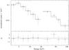 |
Fig. 2 Combined JEM-X1 and ISGRI spectrum of IGR J17451–3022 extracted from the INTEGRAL data in revolution 1458. The best fit model is obtained by using an absorbed power-law model (see text for details). The residuals from the fit are shown in the bottom panel. |
Finally, we also extracted the JEM-X1 and JEM-X2 lightcurves with a time resolution of 2 s to search for type-I X-ray bursts. However, we did not find any significant detection.
3. Swift data
Swift /XRT (Burrows et al. 2005) periodically observed the source starting close to its initial detection until it faded into quiescence 9 months later (i.e., from 2014 August 5 to 2015 June 6). Observations in the period 2014 November to 2015 early February were not available owing to the satellite Sun constraints. A log of all available XRT observations is given in Table 1.
XRT data were collected in both windowed-timing (WT) and photon-counting (PC) mode and analyzed by using standard procedures and the FTOOLS software (v6.16). The XRT data were processed with the xrtpipeline (v.0.13.1) and the latest calibration files available (20140730). The WT data were never affected by pile-up; therefore, WT source events were extracted from circular regions of 20 pixels (1 pixel ~2.36′′). Instead, when required the PC data were corrected for pile-up by adopting standard procedures (Vaughan et al. 2006; Romano et al. 2006). In particular, we determined the size of the affected core of the point spread function (PSF) by comparing the observed and nominal PSF, and excluded all the events that fell within that region from the analysis. The PC source events were thus extracted either from an annuli with an outer radius of 20 pixels and an inner radius determined from the severity of the pile-up, or within circular regions with a radius of 20 pixels when pile-up was not present. Background events were extracted from nearby source-free regions. From each XRT observation we extracted an averaged spectrum and the corresponding barycentered lightcurve. The time resolution of the lightcurves was 1 s for data in WT mode and 2.5 s for data in PC mode. The barycentric correction was applied by using the barycorr tool. For the observations 025–028, a single spectrum was extracted owing to the low statistics of these data. All spectra were binned to ensure at least 20 counts per energy bin and were fit in the 0.5–10 keV energy range.
All XRT spectra could be well fit by using a simple absorbed disk blackbody model (tbabs*diskbb in Xspec; see also Sect. 4). Fits with a power-law model provided in most cases significantly worse results. We report the best fit obtained in all cases in Table 1. The XRT monitoring showed that the spectral energy distribution of the X-ray emission from IGR J17451–3022 was roughly stable along the entire outburst. The absorption column density and the temperature of the thermal component measured by XRT always remained compatible (to within the uncertainties) with the values obtained from the fit to the XMM-Newton data (see Sect. 4). We verified that fixing the XRT absorption column density to the XMM-Newton value would result in acceptable fits to all observations and negligible changes in the temperature of the thermal component. We note that no XRT observations were performed during (or sufficiently close in time to) the INTEGRAL revolution 1458 where a possible spectral state transition of the source was observed (see Sect. 2).
Log of all Swift /XRT observations used in this work.
Given the relatively low statistics of each XRT observation, we did not perform a detailed timing analysis of the data. However, in Fig. 3 we show the total outburst lightcurve of the source as observed by XRT from the onset of the event down to the return in quiescence. In this figure we indicate the time intervals corresponding to the coverage provided by INTEGRAL and the time of the ToO observation carried out by XMM-Newton (see Sect. 4).
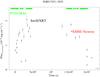 |
Fig. 3 Swift /XRT lightcurve of the entire outburst recorded from IGR J17451–3022. The flux is not corrected for absorption. The start time of the lightcurve (t = 0) is 2014 September 5 at 15:37 (UTC). We also show in the plot the coverage provided by INTEGRAL (see Sect. 2) and the flux measured by XMM-Newton (see Sect. 4). |
4. XMM-Newton data
The XMM-Newton (Jansen et al. 2001) ToO observation of IGR J17451–3022 was performed on 2015 March 06 for a total exposure time of 40 ks. The EPIC-pn was operated in timing mode, the MOS2 in full frame, and the MOS1 in small window. We reduced these data by using the SAS version 14.0 and the latest XMM-Newton calibration files available2 (XMM-CCF-REL-329; see also Pintore et al. 2014). The observation was slightly affected by intervals of high flaring background and thus we filtered out these intervals following the SAS online thread3. The final effective exposure time for the three EPIC cameras was 29 ks.
We first extracted the EPIC-pn lightcurve of the source in the energy range 0.5–12 keV from CCD Cols. 28–46. The corresponding background lightcurve was extracted by using Cols. 3–10. The background-subtracted EPIC-pn lightcurve of IGR J17451–3022 with a time bin of 50 s is shown in Fig. 4; we also used the epiclccorr tool to correct the lightcurves for any relevant instrumental effect. The source displayed an average count-rate of 16 cts s-1, two X-ray eclipses, and the presence of dips at the beginning of the observation and between the two eclipses. Given the source count-rate, both MOS1 and MOS2 data suffered from significant pile-up. This was corrected by following the SAS online threads. The RGS spectra were characterized by a low statistics owing to the significant extinction recorded in the direction of the source (see below). We thus used the RGS and the MOS data only to check the consistency with the results obtained from the analysis of the EPIC-pn data, but do not discuss them in detail. A fit of all data together revealed the presence of instrumental residuals in the EPIC-pn below 1.7 keV (see Fig. 5). This issue has been reported in several papers using the EPIC-pn in timing mode and thus we restricted our spectral analysis to the 1.7–12 keV energy range (see, e.g., Piraino et al. 2012; Pintore et al. 2015; D’Aì et al. 2015; Boirin et al. 2005, for a similar issue with EPIC-pn residuals below 1.7 keV). We barycentered the EPIC-pn data before carrying out any timing analysis.
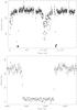 |
Fig. 4 Top: EPIC-pn lightcurve of IGR J17451–3022 (0.5–12 keV). The start time of the lightcurve (t = 0) is 2015 March 6 at 6:26 (UTC). The bin time is 50 s for display purposes. Time intervals with no data are due to the filtering of the high flaring background. Bottom: zoom of the first eclipse (time bin 10 s). The apparent different count-rate at the bottom of the eclipse between this and the upper figure is due to the different time binning. |
4.1. The X-ray eclipses
We used the detection of two consecutive eclipses in the 0.5–12 keV EPIC-pn lightcurve of the source to determine the system orbital period; we used a time bin of 20 s and verified a posteriori that different choices for the time binning would not significantly affect the results. As the eclipses of IGR J17451–3022 are virtually rectangular (see Fig. 4), a fit to each of the two eclipses was carried out using the same technique described by Bozzo et al. (2007) in the case of the eclipsing LMXB 4U 2129+47.
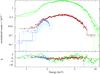 |
Fig. 5 EPIC-pn (green), EPIC-MOS1 (black), EPIC-MOS2 (red), RGS1 (blue), and RGS2 (cyan) average spectra extracted from the XMM-Newton observation of IGR J17451–3022. The model used for the preliminary fit of the data here is an absorbed disk blackbody model (tbabs*diskbb in Xspec). The residuals from the fit in the bottom panel show the instrumental excess in the EPIC-pn data below 1.7 keV (in addition to the many absorption features, see also Fig. 7). For this reason, we only used EPIC-pn data in the energy range 1.7–12 keV for further analysis. |
The model we developed to fit rectangular eclipses treats the mean source count-rate outside (Fmax) and inside (Fmin) the eclipse as free parameters, together with the mid-eclipse epoch (T0) and the duration of the eclipse (D). We performed a minimization of the obtained χ2 value from the fit to the data by using our dedicated IDL routine. The model was integrated over each time bin before computing the χ2 in order to take data binning into account. The routine samples the χ2 hyper-surface in a fine grid of values before computing the variance between the model and the data for each set of parameters. The variance is then used to determine the local χ2 minima in the 4D parameter space. The best fits to the two mid-eclipse epochs were found to be T0(a) = 57087.32320 ± 0.00001 MJD and T0(b) = 57087.5850110 ± 0.00001 MJD. The corresponding eclipse durations were  s and D(b) = 822.66
 s. We show the relevant contour plots for the fits to the two eclipses in Fig. 6. From these measurements, we estimated the orbital period of the system as Porb = 22620.5
 s (all uncertainties here are given at 1σ confidence level). This is a slightly improved measurement compared to the value 22623 ± 5 s reported previously by Jaisawal et al. (2015).
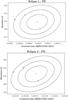 |
Fig. 6 Contour plots of the two eclipses durations and mid-epochs obtained by fitting the rectangular eclipse model to the data. The 1σ, 2σ, and 3σ contours around the best determined values are indicated. |
4.2. Spectral analysis
We first extracted the source spectrum during the steady part of the XMM-Newton observation, i.e., filtering out the time intervals corresponding to the dips and the eclipses (the resulting total exposure time is 16.8 ks). This spectrum showed a curved shape that could be described by using a thermal component typical of an accretion disk (diskbb in Xspec). We accounted for the absorption column density in the direction of the source by using a tbabs component with solar abundances. Although this model could describe the continuum reasonably well, the fit was far from being acceptable (/d.o.f. = 15.94/138) owing to the presence of several absorption features. For completeness, we mention that a fit with an absorbed power law (tbabs*pow in Xspec) would give a significantly worse fit (/d.o.f. = 69.75/138). In Fig. 7 we show the ratio between the data and the model when the fit is carried out by using the tbabs*diskbb model.
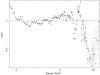 |
Fig. 7 Ratio between the EPIC-pn data and the tbabs*diskbb model. The plot indicates the presence of several absorption features, including a broad structure around ~9 keV. |
In order to improve the fit, we first included a number of absorption Gaussian lines (gaussian in Xspec) to account for all visible features in the residuals, and then included a broad absorption feature (gabs in Xspec) to take into account the deepest structure around ~9 keV (see Fig. 7). We fixed to zero the widths of the lines that could not be constrained after a preliminary fit and left this parameter free to vary in all other cases. This phenomenological fit was used to identify the lines that correspond to known atomic transitions and guide further analysis. We show all the results in Table 2 together with the identification of the lines. We marked with “?” the identifications of the two lines at 5.7 and 6.1 keV for which we did not find any other mention in the literature of LMXBs and that we thus consider tentative associations.
We checked for possible spectral variations by carrying out a time-resolved spectral analysis of the XMM-Newton data, as well as an orbital-phase resolved analysis. The results of the time-resolved spectral analysis are given in Table 2.
Results of the fit to the steady emission from IGR J17451–3022 recorded from XMM-Newton (i.e., excluding the time intervals of the dips and the eclipses).
The results obtained from the orbital phase resolved spectral analysis are given in Table 3. In both cases we could not find evidence of significant spectral variability. We also note that, owing to the reduced statistics of these spectra, obtaining meaningful fits in the 6–8 keV range was particularly challenging because of the blending of several lines.
The spectral analysis of the X-ray dips was carried out separately as the hardness ratio (HR) calculated from the soft (0.5–2.5 keV) and hard (2.5–12.0 keV) X-ray lightcurves of the source as a function of the orbital phase provided clear evidence for spectral variability during these events (see Fig. 8).
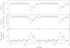 |
Fig. 8 EPIC-pn lightcurve of IGR J17451–3022 folded on the best orbital period determined in this work, |

We extracted orbital phase resolved spectra during phases corresponding to the HR variations: 0.61–0.65, 0.65–0.68, 0.68–0.75, 0.75–0.82, and 0.82–0.85. In all cases a reasonably good fit ( –1.2) could be obtained with an absorbed diskbb model. Owing to the poor statistics of these spectra (integration times of a few ks) we could not measure significant changes in the temperature and radius of the diskbb component or in the absorption column density. Furthermore, several absorption lines appeared as blended and thus we were unable to constrain their parameters in the fits with reasonable accuracy. In order to clarify the origin of the HR increase close to the dips (see Fig. 8), we extracted a single spectrum by combining orbital phases between 0.65 and 0.82. This spectrum revealed a modest (but significant) increase in the column density of both the neutral and the additional ionized absorber. This is discussed further in Sect. 4.2.1.
We also extracted the source spectrum during the two eclipses. Since in this case the source flux was significantly lower, we also made use of the spectra extracted from the two MOS cameras and fit them together with the EPIC-pn. The integration time was too short to obtain meaningful spectra from the two RGSs and so we did not include these data in the combined fit. The spectrum could be equally well fit with an absorbed diskbb (NH = (5.3 ± 0.6) × 1022 cm-2, kT = 1.17 ± 0.09, Ndiskbb = 0.8 ± 0.4,  /d.o.f. = 0.92/98) or a power-law model (NH = (8.8 ± 0.9) × 1022 cm-2, Γ = 3.9 ± 0.3, /d.o.f. = 0.98/98). The measured 0.5–10 keV X-ray flux was 9.5 × 10⁻¹² erg cm-2 s-1. We introduced in the fit inter-calibration constants between the three instruments and found them to be compatible with unity (to within the uncertainties).
4.2.1. Physical spectral model
The spectral properties of the source analyzed in Sect. 4.2, together with the characteristics of the lightcurve discussed in Sect. 4.1, are strongly reminiscent of high inclination LMXBs with absorbing/outflowing material located above the accretion disk (see Sect. 5). In order to provide a more physical description of the spectral energy distribution of IGR J17451–3022, we made use of a model comprising a diskbb component which is affected by both the Galactic absorption and a local “warm” absorber (warmabs4 in Xspec). This model takes into account the ionization status of the gas, its turbulent broadening velocity, its bulk velocity (through the measurement of redshifted or blueshifted lines), and the abundance of the different materials with respect to solar values. Following the identification of several absorption lines in Sect. 4.2, we left the abundances corresponding to Si, S, Ar, Ca, Mn, K, and Fe free to vary in the fit. A cabs component that accounts for Compton scattering (not included in warmabs) was also added to the fit. We fixed the column density of this component to be the same as the warbmabs multiplied by a factor of 1.21 to take roughly into account the number of electrons per hydrogen atom (in the case of solar abundances; see, e.g., Díaz Trigo et al. 2014, and references therein). We changed the default ionizing continuum in warmabs, which is a power-law of photon index Γ = 2, to a blackbody ionizing continuum with kT ~ 1.2 keV. Even though the source might undergo some spectral state transitions characterized by a non-thermal power-law component, this does not seem to be the case for most of the outburst (see Sect. 2). As it is not possible to select a diskbb component as an ionizing continuum in the warmabs model, we chose the available blackbody continuum with a similar temperature because it was a reasonably good approximation in the case of IGR J17451–3022 (as was also done in other sources, see, e.g., Díaz Trigo & Boirin 2013). We also assumed 1012 cm-3 for the ionized medium density, a value typically used in LMXBs (see, e.g., Díaz Trigo et al. 2014). The drop in the source X-ray emission at energies ≳9 keV that required the addition of a gabs component in the phenomenological model was completely accounted for by the addition of the warmabs model. We included an additional edge at ~8.2 keV in the fit to minimize the residuals still visible around this energy and two absorption Gaussian lines with centroid energies of ~5.7 keV and ~6.1 keV. These two lines improved the fit to the Cr and Mn lines, which were not fully taken into account by the warmabs component. This model provided an acceptable result (see Table 4). The residuals left from this fit did not suggest the presence of additional spectral components, even though some structures remained visible close to the iron lines at 6.7–7.0 keV (see Fig. 9). These structures might result from a non-optimal description of the complex absorbing medium in IGR J17451–3022 through the warmabs model, e.g., due to the presence of different broadening or outflowing velocities.
We used the best fit model also to characterize the spectrum extracted during the orbital phases corresponding to the dips and the most evident HR variations (0.65–0.72 and 0.72–0.82; see Sect. 4.2). This allowed a more physical comparison between the average emission of the source and the emission during the dips. Owing to the reduced statistics of the dip spectrum, we fixed in the fit those parameters that could not be constrained to the values determined from the average spectrum. The results of this fit, summarized in Table 4, suggest that the dips are likely caused by a moderate (but significant) increase in the column density of the neutral and ionized absorber close to the source.
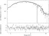 |
Fig. 9 Best fit to the average EPIC-pn spectrum of the steady emission from IGR J17451–3022 (excluding the time intervals corresponding to the eclipses and the dips) with the physical model described in Sect. 4.2.1. We show here the unfolded spectrum. The residuals from the fit are shown in the bottom panel. |
4.3. Timing analysis
We also performed a timing analysis of the EPIC-pn data to search for coherent signals. We first reported all photons arrival times to the solar system barycentre using the Chandra position of the source (see Sect. 1). The orbital motion of the compact object limits the length of the time series over which a search for periodicities can be performed without taking into account the Doppler shift induced by the motion of the source. To evaluate this time interval we calculated Eq. (21) of Johnston & Kulkarni (1991) for an orbital period of Porb = 6.28 h and an inclination i ~ 80°, obtaining  (1)Assuming the case of a signal with a putative frequency of ν = 300 Hz, described by m = 1 harmonic and emitted by an object orbiting around a M2 ~ 0.3 M⊙ companion star (Zdziarski et al. 2016), we then calculated a Fourier power spectrum in intervals of length Δtbest = 448.6 s. The time series was sampled at eight times the minimum time resolution of the timing mode of the EPIC-pn (tres = 2.952 × 10⁻⁵ s), obtaining a value of the Nyquist frequency, νNy = (8tres)-1/ 2 = 2117 Hz. We then inspected frequencies up to νNy (with a frequency resolution of
  Hz) to search for a coherent periodic signal, but found none significant with an upper limit on the pulse amplitude of A< 12.5% (3σ confidence level).
In order to improve the sensitivity to pulsed signals emitted by a source in a binary system, we used a quadratic coherence recovery technique (QCRT) following the guidelines given by Wood et al. (1991) and Vaughan et al. (1994). This technique is based on the correction of the photon arrival times with a quadratic transformation, under the assumption that the sinusoidal Doppler modulation introduced by the orbital motion can be approximated by a parabola over a time interval that is short enough. To estimate such a length we calculated Eq. (22) of Johnston & Kulkarni (1991) for the same parameters mentioned above:  (2)In order to increase the speed of the power spectrum calculation, we considered a value of the interval length equal to a power of two of the time resolution of the time series, Δtbest = 226tres = 1981, and divided the time series into Nintv = 20 intervals. Before performing a signal search, the arrival times of the X-ray photons in each of these intervals were corrected using a quadratic relation t′ = αt2. The parameter α was varied in steps equal to
 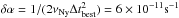 within a range determined by considering the possible size of the two components. Calculating the expression given by Wood et al. (1991) for Porb = 6.28 h, we considered αmax = αmin = 1.54 × 10⁻⁷ [ M2/ (M1 + M2) ] [ (M1 + M2) /M⊙ ] 1/3s-1. Assuming as example values M1 = 1.7 M⊙, and M2 = 0.3 M⊙, we obtained αmax = αmin = 2.9 × 10⁻⁸ s. The number of corrections made to the preliminary arrival times for each of the Nintv = 20 time intervals is then Nα = 2αmax/δα = 967. A power spectrum was produced for each of these trial corrections, inspecting frequencies up to νNy = (8tres)-1/ 2 = 2117 Hz with a resolution of δν = 1/Δtbest = 1/(226tres) = 5 × 10⁻⁴ Hz, giving a total number of frequency trials equal to Nν = νNy/δν = 222. The total number of trials is then NintvNαNν = 8.1 × 10¹⁰, and assuming that in the absence of any signal the noise in the power spectrum is distributed as a χ2 with two degrees of freedom, we then set a post-trial detection level at 3σ confidence level of Pdet = 62.1. No signal was significantly detected and upper limits of ≃5% (3σ confidence level) were typically found in the different time intervals.
5. Discussion
We reported on the analysis of the X-ray data collected during the first outburst of the INTEGRAL transient IGR J17451–3022. The source displayed a relatively soft X-ray emission during most of the event (lasting about 9 months) and thus it was not significantly detected by the hard X-ray imager IBIS/ISGRI on board INTEGRAL. The only exception is the time interval corresponding to the satellite revolution 1458 where the source underwent a possible spectral state transition and its X-ray emission was recorded up to ~100 keV. During the INTEGRAL revolution 1458, the spectrum of the source could be described well by using a relatively hard power law with a photon index of Γ ~ 2. During all the remaining outburst phases covered by INTEGRAL the source was only significantly detected by JEM-X at energies ≲10 keV. The average JEM-X spectrum, however, was characterized by low statistics and did not permit a clear distinction between different possible spectral models. The JEM-X data showed, nevertheless, that the X-ray flux of the source remained relatively stable in the 3–10 keV energy band and was compatible with that recorded by Swift /XRT before the beginning of the outburst decay.
The Swift /XRT observations covered a large part of the source outburst, excluding the time period 2014 November to 2015 February when the visibility of the Galactic center was limited by Sun constraints. The XRT data did not reveal any dramatic spectral change in the X-ray emission from the source during the outburst. Its spectrum was dominated by a thermal component, interpreted as being due to the presence of an accretion disk. The hard X-ray emission recorded during the INTEGRAL revolution 1458 could thus have been due to a temporary spectral state transition of the source, similar to what is often observed during the outbursts of neutron star (NS) and black hole (BH) LMXBs (see, e.g., Done et al. 2007; Muñoz-Darias et al. 2014, for recent reviews). Owing to the lack of simultaneous coverage with focusing X-ray instruments during the INTEGRAL revolution 1458 and the availability of spectra with sufficiently high statistics, we were not able to investigate this possible spectral state transition in greater detail.
The same spectral component that dominated all XRT spectra was also detected in the XMM-Newton observation of the source carried out in 2015 March. The EPIC data clearly showed the presence of a number of absorption features, the most evident ones being centered at the known energies of the Fe XXV/Fe XXVI Kα and Kβ complexes. Similar features are observed in a number of LMXBs hosting either a NS or a BH, and are usually ascribed to the presence of an ionized absorbing material located above the accretion disk (Ueda et al. 1998; Kotani et al. 2000; Sidoli et al. 2001; Parmar et al. 2002; Boirin & Parmar 2003; Boirin et al. 2004, 2005; Hyodo et al. 2008). Such absorbers are more likely to be observed in high inclination systems (≳70 deg; see, e.g., Ponti et al. 2012, 2014; D’Aì et al. 2014) where our line of sight passes directly through the disk. In some cases, the absorption features show significant blueshifts, thus indicating that the ionized material is emerging from the system as a “disk wind” (see, e.g., Schulz & Brandt 2002; Kubota et al. 2007; Díaz Trigo et al. 2007; Iaria et al. 2008). Different driving mechanisms that generate disk winds have been proposed (see, e.g., Proga & Kallman 2002). These comprise a combination of radiation and thermal pressure, best suited to explain disk winds forming at distances of ≳1010–1012 cm from the central compact object, or magnetic effects. In the latter case the disk wind can be produced at relatively small distances from the compact object (≲109–1010 cm) owing to the pressure generated by the magnetic viscosity internal to the disk or magnetocentrifugal forces (Miller et al. 2006). In all cases, the presence of an ionized absorbing material can be accounted for in the spectral analysis of high inclination LMXBs by using the warmabs model in Xspec. The fit with this model that we carried out on the IGR J17451–3022 data in Sect. 4.2.1 revealed that the warm absorber in this source has a column density of  cm-2, a turbulent velocity of σv ≃ 290 km s-1, and a bulk velocity v ≃ 2200 km s-1. The last value indicates that this material is moving away from the disk and can thus be most likely associated with a disk wind. We note here that even though the measured outflowing velocity in Table 4 is highly significant, the corresponding shift in energy of the involved lines is modest (about 0.7% of the centroid energy) and is roughly of the same order of magnitude as the EPIC-pn calibration energy accuracy. For this reason, any interpretation of the presence of an outflowing velocity on the order of a few thousand km s-1 measured with the EPIC-pn has to be taken with caution.
From the estimated column density and ionization parameter of the warm absorber, we can also infer the distance of this material from the compact object by using the definition of the ionization parameters ξ = LX/ner2, where LX is the source X-ray luminosity, ne ≃ 1012 cm-3 is the medium density assumed in the warmabs model, and r is the distance between the absorbing medium and the central source. Making use of the best fit values in Table 4, we obtain r ≃ 2.0 × 1010 cm, which is an intermediate value of the ionized absorber distance from the central compact object dividing thermal/radiative and magnetic models.
We caution, however, that the distance to IGR J17451–3022 is not known at present (thus potentially leading to large uncertainties on the estimated X-ray luminosity of the source) and that the above calculation depends on the density assumed for the partly ionized absorbing medium (see Sect. 4.2.1). Disk winds are usually observed in bright LMXBs hosting a BH in the radio-free high soft state (HSS) or a NS with a luminosity LX ≳ 0.15LEdd (here LEdd is the Eddington luminosity for an accreting NS; see, e.g., Ponti et al. 2012, 2014, 2015, and references therein). The X-ray luminosity estimated from the unabsorbed XMM-Newton flux of IGR J17451–3022 is LX ≃ 4.3 × 1036(D/ 8 kpc)2 erg s-1, i.e., about 2% of the typical Eddington luminosity for a NS and a relatively low luminosity for a Galactic BH in the HSS (see, e.g., Done et al. 2007, for a recent review). This suggests that IGR J17451–3022 might be located well beyond the Galactic Center, i.e., at distances ≫8 kpc. The lack of optical/radio/IR observations during the outburst of IGR J17451–3022 (to the best of our knowledge) currently prevents a more accurate estimate of the source distance. We note that, as it occurs in other sources seen at high inclination, it is also possible that only a fraction of the intrinsic X-ray luminosity arrives to the observer (see, e.g., Burderi et al. 2010), thus increasing our uncertainty concerning the source localization and the interpretation on its real nature. Concerning the assumed value of ne, we commented in Sect. 4.2.1 that ~1012 cm-3 is a reasonable estimate based on our knowledge of similar systems. Direct measurements of the plasma density in LMXBs displaying the presence of pronounced absorption features has only been obtained in two cases so far, and thus we cannot rule out substantially different values of ne (see Díaz Trigo & Boirin 2015, and references therein).
At odds with other LMXBs seen at high inclinations and characterized by dense coronae (see, e.g., Díaz Trigo & Boirin 2013), we find no evidence for either a broad iron emission line or a reflection component produced close to the inner disk boundary in IGR J17451–3022. The prominence of these features is a strong function of the system inclination and might become undetectable at ≳80 deg (see, e.g., García et al. 2014). We find evidence for an edge at ~8.2 keV (see Table 4) that could be due to Fe XXV, even though the measured energy is lower than expected (8.828 keV; see, e.g., di Salvo et al. 2009, for a similar case). An alternative possibility is that the residuals around this energy are left due to a poor fit with the warmabs model, especially in an energy range where the effective area of the EPIC-pn camera is decreasing rapidly and the signal-to-noise ratio of the data is far from being optimal (see Fig. 9).
The analysis of the EPIC-pn data has also revealed the presence of two virtually rectangular eclipses in the source lightcurve, lasting about 820 s each. From the measurement of the two eclipse mid-epochs we provided an estimate of the source orbital period at 22620.5 s (1σ confidence level; see Sect. 4.1). The residual X-ray flux measured during the eclipses (about 6% of the averaged uneclipsed flux) could in principle be explained by the presence of an accretion disk corona (ADC) located above the disk that scatters the X-rays from the central point-like source. However, as the X-ray spectrum extracted during the eclipse could be equally well fit with a diskbb or a power-law model, we are unable to determine whether this residual emission corresponds to a fraction of the scattered thermal X-rays from the disk or whether there is also some significant reprocessing within the ADC with an eventual contribution from a scattering halo. This phenomenology is remarkably similar to that observed in the case of the NS LMXB EXO 0748-676, which shows rectangular eclipses with a 4% residual X-ray flux (during X-ray active periods; see, e.g., Parmar & White 1988).
The X-ray dips detected by XMM-Newton from IGR J17451–3022 also show remarkable similarities with the dips in EXO 0748-676. In both systems, the dips precede the X-ray eclipse in phase and display complex structures varying from one orbit to the other. They also give rise to measurable changes in the hardness ratio of the source emission, which is interpreted in terms of increased absorption due to the presence of vertically extended structures in the disk at the impact point of the accretion stream from the donor star. It is worth noting that EXO 0748-676 also displayed clear evidence of an ionized absorbing material located above the accretion disk, even though no significant blueshift of the detected absorption features could be measured in that case (Ponti et al. 2014).
Both the search for X-ray bursts and for pulsations resulted in non-detections, leaving the nature of the compact object in IGR J17451–3022 unclear (see Sect. 2 and 4.3). As disk winds are currently understood to be a ubiquitous property of many NS and BH LMXBs observed at high inclination, this feature cannot be used to distinguish easily between the two possibilities in the case of IGR J17451–3022. The analysis of the X-ray continuum from the source could, however, provide some additional clues. In particular, the normalization of the diskbb model in the XMM-Newton and Swift data is found always to be ≲20 and thus we can infer an approximate inner disk boundary of 12(d/ 8 kpc)(cos(θ/ 85 deg))(− 1/2) km. Even when the usual color and torque-free boundary corrections are considered for the diskbb component (see, e.g., Gierliński et al. 1999; Nowak et al. 2012, and references therein), the inner disk boundary estimated from the X-ray spectrum of IGR J17451–3022 remains uncomfortably small for a black hole (less than 2 rg for a 3 M⊙ BH). Although this does not allow us to draw a firm conclusion about the nature of the compact object in IGR J17451–3022, we conclude that the NS hypothesis is favoured (see also Zdziarski et al. 2016).
The conversion from count-rate to mCrab was carried out by using the most recent observations of the Crab (at the time of writing) in spacecraft revolution 1597. From these data we measured a count-rate for the Crab of 139.4 cts s-1 and 75.2 cts s-1 from the IBIS/ISGRI mosaics in the 20–40 keV and 40–80 keV bands. The estimated count-rates in the JEM-X mosaics were of 111.6 cts s-1 and 29.6 cts s-1 in the energy band 3–10 keV and 10–20 keV, respectively.
Acknowledgments
We thank N. Schartel and the XMM-Newton team for having promptly performed the ToO observation analyzed in this paper. We are indebted to the Swift PI and operations team for the continuous support during the monitoring campaign of X-ray transients. We thank an anonymous referee for the useful comments. A.A.Z. and P.P. have been supported in part by the Polish NCN grants 2012/04/M/ST9/00780 and 2013/10/M/ST9/00729. A.P. is supported by a Juan de la Cierva fellowship, and acknowledges grants AYA2012-39303, SGR2009-811, and iLINK2011-0303. P.R. acknowledges contract ASI-INAF I/004/11/0. G.P. acknowledges support by the Bundesministerium für Wirtschaft und Technologie/Deutsches Zentrum für Luft- und Raumfahrt (BMWI/DLR, FKZ 50 OR 1408) and the Max Planck Society. L.B. e T.D. acknowledge contract ASI-INAF.
References
- Altamirano, D., Wijnands, R., Heinke, C. O., & Bahramian, A. 2014, ATel, 6469, 1 [NASA ADS] [Google Scholar]
- Bahramian, A., Heinke, C. O., Beardmore, A. P., Altamirano, D., & Wijnands, R. 2014a, ATel, 6501, 1 [NASA ADS] [Google Scholar]
- Bahramian, A., Heinke, C. O., Wijnands, R., & Altamirano, D. 2014b, ATel, 6486, 1 [NASA ADS] [Google Scholar]
- Bahramian, A., Heinke, C. O., Altamirano, D., & Wijnands, R. 2015a, ATel, 7570, 1 [NASA ADS] [Google Scholar]
- Bahramian, A., Heinke, C. O., Wijnands, R., & Altamirano, D. 2015b, ATel, 7028, 1 [NASA ADS] [Google Scholar]
- Boirin, L., & Parmar, A. N. 2003, A&A, 407, 1079 [NASA ADS] [CrossRef] [EDP Sciences] [Google Scholar]
- Boirin, L., Parmar, A. N., Barret, D., Paltani, S., & Grindlay, J. E. 2004, A&A, 418, 1061 [NASA ADS] [CrossRef] [EDP Sciences] [Google Scholar]
- Boirin, L., Méndez, M., Díaz Trigo, M., Parmar, A. N., & Kaastra, J. S. 2005, A&A, 436, 195 [NASA ADS] [CrossRef] [EDP Sciences] [Google Scholar]
- Bozzo, E., Falanga, M., Papitto, A., et al. 2007, A&A, 476, 301 [NASA ADS] [CrossRef] [EDP Sciences] [Google Scholar]
- Burderi, L., Di Salvo, T., Riggio, A., et al. 2010, A&A, 515, A44 [NASA ADS] [CrossRef] [EDP Sciences] [Google Scholar]
- Burrows, D. N., Hill, J. E., Nousek, J. A., et al. 2005, Space Sci. Rev., 120, 165 [NASA ADS] [CrossRef] [Google Scholar]
- Chakrabarty, D., Jonker, P. G., & Markwardt, C. B. 2014, ATel, 6533, 1 [NASA ADS] [Google Scholar]
- Chenevez, J., Vandbaek Kroer, L., Budtz-Jorgensen, C., et al. 2014, ATel, 6451, 1 [NASA ADS] [Google Scholar]
- Courvoisier, T., Walter, R., Beckmann, V., et al. 2003, A&A, 411, L53 [NASA ADS] [CrossRef] [EDP Sciences] [Google Scholar]
- D’Aì, A., Iaria, R., Di Salvo, T., et al. 2014, A&A, 564, A62 [NASA ADS] [CrossRef] [EDP Sciences] [Google Scholar]
- D’Aì, A., Di Salvo, T., Iaria, R., et al. 2015, MNRAS, 449, 4288 [NASA ADS] [CrossRef] [Google Scholar]
- di Salvo, T., D’Aí, A., Iaria, R., et al. 2009, MNRAS, 398, 2022 [NASA ADS] [CrossRef] [Google Scholar]
- DíazTrigo, M., & Boirin, L. 2013, Acta Polytechnica, 53, 659 [Google Scholar]
- Díaz Trigo, M., & Boirin, L. 2015, Astronomical Notes, submitted [arXiv:1510.03576] [Google Scholar]
- Díaz Trigo, M., Parmar, A. N., Miller, J., Kuulkers, E., & Caballero-García, M. D. 2007, A&A, 462, 657 [NASA ADS] [CrossRef] [EDP Sciences] [Google Scholar]
- Díaz Trigo, M., Migliari, S., Miller-Jones, J. C. A., & Guainazzi, M. 2014, A&A, 571, A76 [NASA ADS] [CrossRef] [EDP Sciences] [Google Scholar]
- Done, C., Gierliński, M., & Kubota, A. 2007, A&ARv, 15, 1 [NASA ADS] [CrossRef] [EDP Sciences] [Google Scholar]
- García, J., Dauser, T., Lohfink, A., et al. 2014, ApJ, 782, 76 [NASA ADS] [CrossRef] [Google Scholar]
- Gierliński, M., Zdziarski, A. A., Poutanen, J., et al. 1999, MNRAS, 309, 496 [NASA ADS] [CrossRef] [Google Scholar]
- Heinke, C. O., Bahramian, A., Altamirano, D., & Wijnands, R. 2014, ATel, 6459, 1 [NASA ADS] [Google Scholar]
- Hyodo, Y., Ueda, Y., Yuasa, T., et al. 2008, ArXiv e-prints [arXiv:0809.1278] [Google Scholar]
- Iaria, R., D’Aí, A., Lavagetto, G., et al. 2008, ApJ, 673, 1033 [NASA ADS] [CrossRef] [Google Scholar]
- Jaisawal, G. K., Homan, J., Naik, S., & Jonker, P. 2015, ATel, 7361, 1 [NASA ADS] [Google Scholar]
- Jansen, F., Lumb, D., Altieri, B., et al. 2001, A&A, 365, L1 [NASA ADS] [CrossRef] [EDP Sciences] [Google Scholar]
- Johnston, H. M., & Kulkarni, S. R. 1991, ApJ, 368, 504 [NASA ADS] [CrossRef] [Google Scholar]
- Kotani, T., Ebisawa, K., Dotani, T., et al. 2000, ApJ, 539, 413 [NASA ADS] [CrossRef] [Google Scholar]
- Kubota, A., Dotani, T., Cottam, J., et al. 2007, PASJ, 59, 185 [NASA ADS] [Google Scholar]
- Lebrun, F., Leray, J. P., Lavocat, P., et al. 2003, A&A, 411, L141 [NASA ADS] [CrossRef] [EDP Sciences] [Google Scholar]
- Lund, N., Budtz-Jørgensen, C., Westergaard, N. J., et al. 2003, A&A, 411, L231 [NASA ADS] [CrossRef] [EDP Sciences] [Google Scholar]
- Miller, J. M., Raymond, J., Fabian, A., et al. 2006, Nature, 441, 953 [NASA ADS] [CrossRef] [PubMed] [Google Scholar]
- Muñoz-Darias, T., Fender, R. P., Motta, S. E., & Belloni, T. M. 2014, MNRAS, 443, 3270 [NASA ADS] [CrossRef] [Google Scholar]
- Nowak, M. A., Wilms, J., Pottschmidt, K., et al. 2012, ApJ, 744, 107 [NASA ADS] [CrossRef] [Google Scholar]
- Parmar, A. N., & White, N. E. 1988, Mem. Soc. Astron. It., 59, 147 [NASA ADS] [Google Scholar]
- Parmar, A. N., Oosterbroek, T., Boirin, L., & Lumb, D. 2002, A&A, 386, 910 [NASA ADS] [CrossRef] [EDP Sciences] [Google Scholar]
- Pintore, F., Sanna, A., Di Salvo, T., et al. 2014, MNRAS, 445, 3745 [NASA ADS] [CrossRef] [Google Scholar]
- Pintore, F., Di Salvo, T., Bozzo, E., et al. 2015, MNRAS, 450, 2016 [NASA ADS] [CrossRef] [Google Scholar]
- Piraino, S., Santangelo, A., Kaaret, P., et al. 2012, A&A, 542, L27 [NASA ADS] [CrossRef] [EDP Sciences] [Google Scholar]
- Ponti, G., Fender, R. P., Begelman, M. C., et al. 2012, MNRAS, 422, L11 [NASA ADS] [CrossRef] [Google Scholar]
- Ponti, G., Muñoz-Darias, T., & Fender, R. P. 2014, MNRAS, 444, 1829 [NASA ADS] [CrossRef] [Google Scholar]
- Ponti, G., Bianchi, S., Muñoz-Darias, T., et al. 2015, MNRAS, 446, 1536 [NASA ADS] [CrossRef] [Google Scholar]
- Proga, D., & Kallman, T. R. 2002, ApJ, 565, 455 [NASA ADS] [CrossRef] [Google Scholar]
- Romano, P., Campana, S., Chincarini, G., et al. 2006, A&A, 456, 917 [NASA ADS] [CrossRef] [EDP Sciences] [Google Scholar]
- Schulz, N. S., & Brandt, W. N. 2002, ApJ, 572, 971 [NASA ADS] [CrossRef] [Google Scholar]
- Sidoli, L., Oosterbroek, T., Parmar, A. N., Lumb, D., & Erd, C. 2001, A&A, 379, 540 [NASA ADS] [CrossRef] [EDP Sciences] [Google Scholar]
- Ubertini, P., Lebrun, F., Di Cocco, G., et al. 2003, A&A, 411, L131 [NASA ADS] [CrossRef] [EDP Sciences] [Google Scholar]
- Ueda, Y., Inoue, H., Tanaka, Y., et al. 1998, ApJ, 492, 782 [NASA ADS] [CrossRef] [Google Scholar]
- Vaughan, B. A., van der Klis, M., Wood, K. S., et al. 1994, ApJ, 435, 362 [NASA ADS] [CrossRef] [Google Scholar]
- Vaughan, S., Goad, M. R., Beardmore, A. P., et al. 2006, ApJ, 638, 920 [NASA ADS] [CrossRef] [Google Scholar]
- Wood, K. S., Norris, J. P., Hertz, P., et al. 1991, ApJ, 379, 295 [NASA ADS] [CrossRef] [Google Scholar]
- Zdziarski, A. A., Ziolkowski, J., Bozzo, E., & Pjanka, P. 2016, A&A, submitted [arXiv:1603.07288] [Google Scholar]
All Tables
Results of the fit to the steady emission from IGR J17451–3022 recorded from XMM-Newton (i.e., excluding the time intervals of the dips and the eclipses).
All Figures
|
Fig. 1 INTEGRAL JEM-X mosaicked image around the position of IGR J17451–3022 (3–10 keV). This was obtained by using the data collected during the satellite revolutions 1448–1533 (excluding 1458; see text for details). The source is detected in this mosaic with a significance of 23.7σ. |
| In the text | |
|
Fig. 2 Combined JEM-X1 and ISGRI spectrum of IGR J17451–3022 extracted from the INTEGRAL data in revolution 1458. The best fit model is obtained by using an absorbed power-law model (see text for details). The residuals from the fit are shown in the bottom panel. |
| In the text | |
|
Fig. 3 Swift /XRT lightcurve of the entire outburst recorded from IGR J17451–3022. The flux is not corrected for absorption. The start time of the lightcurve (t = 0) is 2014 September 5 at 15:37 (UTC). We also show in the plot the coverage provided by INTEGRAL (see Sect. 2) and the flux measured by XMM-Newton (see Sect. 4). |
| In the text | |
|
Fig. 4 Top: EPIC-pn lightcurve of IGR J17451–3022 (0.5–12 keV). The start time of the lightcurve (t = 0) is 2015 March 6 at 6:26 (UTC). The bin time is 50 s for display purposes. Time intervals with no data are due to the filtering of the high flaring background. Bottom: zoom of the first eclipse (time bin 10 s). The apparent different count-rate at the bottom of the eclipse between this and the upper figure is due to the different time binning. |
| In the text | |
|
Fig. 5 EPIC-pn (green), EPIC-MOS1 (black), EPIC-MOS2 (red), RGS1 (blue), and RGS2 (cyan) average spectra extracted from the XMM-Newton observation of IGR J17451–3022. The model used for the preliminary fit of the data here is an absorbed disk blackbody model (tbabs*diskbb in Xspec). The residuals from the fit in the bottom panel show the instrumental excess in the EPIC-pn data below 1.7 keV (in addition to the many absorption features, see also Fig. 7). For this reason, we only used EPIC-pn data in the energy range 1.7–12 keV for further analysis. |
| In the text | |
|
Fig. 6 Contour plots of the two eclipses durations and mid-epochs obtained by fitting the rectangular eclipse model to the data. The 1σ, 2σ, and 3σ contours around the best determined values are indicated. |
| In the text | |
|
Fig. 7 Ratio between the EPIC-pn data and the tbabs*diskbb model. The plot indicates the presence of several absorption features, including a broad structure around ~9 keV. |
| In the text | |
|
Fig. 8 EPIC-pn lightcurve of IGR J17451–3022 folded on the best orbital period determined in this work, |
| In the text | |
|
Fig. 9 Best fit to the average EPIC-pn spectrum of the steady emission from IGR J17451–3022 (excluding the time intervals corresponding to the eclipses and the dips) with the physical model described in Sect. 4.2.1. We show here the unfolded spectrum. The residuals from the fit are shown in the bottom panel. |
| In the text | |
Current usage metrics show cumulative count of Article Views (full-text article views including HTML views, PDF and ePub downloads, according to the available data) and Abstracts Views on Vision4Press platform.
Data correspond to usage on the plateform after 2015. The current usage metrics is available 48-96 hours after online publication and is updated daily on week days.
Initial download of the metrics may take a while.