| Issue |
A&A
Volume 589, May 2016
|
|
|---|---|---|
| Article Number | A129 | |
| Number of page(s) | 15 | |
| Section | Planets and planetary systems | |
| DOI | https://doi.org/10.1051/0004-6361/201527344 | |
| Published online | 26 April 2016 | |
Effect of turbulence on collisions of dust particles with planetesimals in protoplanetary disks
1
Laboratoire J.-L. Lagrange, Université Côte d’Azur, Observatoire de la Côte
d’Azur, CNRS,
06304
Nice,
France
e-mail:
This email address is being protected from spambots. You need JavaScript enabled to view it.
2
Anton Pannekoek Institute for Astronomy, University of
Amsterdam, 1012
WX
Amsterdam, The
Netherlands
3
Department of Earth and Planetary Sciences, Tokyo Institute of
Technology, 152-8551
Tokyo,
Japan
4
Earth-Life Science Institute, Tokyo Institute of
Technology, 152-8550
Tokyo,
Japan
Received: 11 September 2015
Accepted: 29 January 2016
Abstract
Context. Planetesimals in gaseous protoplanetary disks may grow by collecting dust particles. Hydrodynamical studies show that small particles generally avoid collisions with the planetesimals because they are entrained by the flow around them. This occurs when St, the Stokes number, defined as the ratio of the dust stopping time to the planetesimal crossing time, becomes much smaller than unity. However, these studies have been limited to the laminar case, whereas these disks are believed to be turbulent.
Aims. We want to estimate the influence of gas turbulence on the dust-planetesimal collision rate and on the impact speeds.
Methods. We used three-dimensional direct numerical simulations of a fixed sphere (planetesimal) facing a laminar and turbulent flow seeded with small inertial particles (dust) subject to a Stokes drag. A no-slip boundary condition on the planetesimal surface is modeled via a penalty method.
Results. We find that turbulence can significantly increase the collision rate of dust particles with planetesimals. For a high turbulence case (when the amplitude of turbulent fluctuations is similar to the headwind velocity), we find that the collision probability remains equal to the geometrical rate or even higher for St ≳ 0.1, i.e., for dust sizes an order of magnitude smaller than in the laminar case. We derive expressions to calculate impact probabilities as a function of dust and planetesimal size and turbulent intensity.
Key words: planets and satellites: formation / planet-disk interactions / turbulence / accretion, accretion disks / hydrodynamics / methods: numerical
© ESO, 2016
1. Introduction
Conventional models for planet formation involve the hierarchical growth by accretion of “planetesimals”. Such building blocks undergo collisions and gravitational binding to eventually reach planetary sizes (see, e.g., Safronov 1972; Hayashi et al. 1985). Still several serious uncertainties remain in the processes leading from sub-μm dust grains, which follow the sub-Keplerian gas, to km-sized planetesimals that are massive enough to move on Keplerian orbits. One of them is known as the “meter-size barrier”. Meter-sized bodies experience a strong drag force, which causes rapid orbital decay due to angular momentum loss. The timescale of this decay is less than 100 yr at 1 AU (see, e.g., Weidenschilling 1984; Nakagawa et al. 1986), which is shorter by several orders of magnitude than the observationally inferred disk lifetime (several million years). Consequently, the planet-forming material are lost from the disk.
One scenario for overcoming the meter-size barrier is by the combined effect of streaming instabilities and pebble accretion. Because of growth to mm/cm-sized particles and settling, dust concentrates in the midplane and may become unstable to streaming instabilities (Youdin & Goodman 2005; Johansen et al. 2007, 2011). This forms relatively large planetesimals. After that, these large planetesimals can sweep up surrounding grains and migrating pebbles (Ormel & Klahr 2010; Ormel & Kobayashi 2012; Lambrechts & Johansen 2012). Because the orbital decay of the pebbles is also fast, a large number of pebbles are supplied from outer disk regions on relatively short timescales, resulting in rapid planet growth. This scenario utilizes the too rapid migration problem, rather than avoids it. The pebble accretion model is actively discussed for the formation of the solar system (Morbidelli et al. 2015) and of close-in super-Earth systems in exoplanetary systems (Chatterjee & Tan 2014, 2015). However, the details of the accretion of grains and pebbles by (large) planetesimals have not been fully clarified.
Guillot et al. (2014) proposed detaile expressions for the accretion rates of dust grains in a protoplanetary gaseous disk for a wide range of dust and planetesimal sizes. They point out that, when using the numerical results by Sekiya & Takeda (2003), the accretion probability drops off by several orders of magnitude at relatively small dust grains (within what they refer to as the “hydrodynamical regime”). This strong depletion can be easily explained by qualitative physical arguments. The motion of small grains is strongly coupled to the gas flow. Since they follow gas streamlines they may avoid (head-on) collisions with the planetesimal. However, the numerical simulations by Sekiya & Takeda (2003) assume laminar flow, while it is known that the disk gas is most likely to be turbulent. Observationally inferred accretion rate in T-Tauri disks is far higher than that caused by molecular viscosity. Consequently, protoplanetary disks are expected to be turbulent, with a turbulent eddy viscosity νt much higher than the molecular kinematic viscosity. Turbulence should affect the reduction in the dust accretion probability in hydrodynamical regime. Recently, Mitra et al. (2013) studied the influence of turbulence on the dust impact velocity by means of two-dimensional direct numerical simulations. They found a velocity distribution with exponential tails and argued that most of the dust collides with a speed comparable to that of the head wind.
The purpose of this paper is to propose expressions for dust accretion probabilities on planetesimals in turbulent gas, based on three-dimensional direct hydrodynamical simulations. Gravity effects are omitted in this study and are left for a future work. We follow the approach introduced by Homann & Bec (2015) and consider an idealized situation in which the planetesimal is assumed to be spherical with a smooth surface. The gas is modeled as a purely hydrodynamical and incompressible fluid so that other possible modes originating from either the magneto-rotational instability (MRI) or compressibility are not taken into account. Additionally, we neglect any shear, disregard gravitational effects, and do not allow for rotation of the planetesimal. The aim of this work is twofold: first, it shall provide a detailed study of collisions between small inertial grains and a large spherical object and, secondly, it shall determine its consequences on the accretion of dust by planetesimals in the context of planet formation.
It is worth mentioning that our results, involving the hydrodynamical interactions and the collisions between a large spherical inclusion and small particles with inertia, have important applications in contexts that go beyond planet formation. In atmospheric physics, this problem is known as “inertial impaction” and is relevant for estimating rates in rain formation or wet deposition of aerosols where a falling water drop scavenges smaller cloud droplets or solid pollutants. Studies of such problems often rely on collision efficiencies and, again, mainly formulas from laminar flow conditions are used (Berthet et al. 2010). A popular formula is that of Slinn (1974), who proposed a fit of the collision efficiency for the inertial impaction regime. Later, he included molecular diffusion and extended his formula to smaller projectiles (Slinn 1976, 1983). Inertial impaction is also important for the design and improvement of industrial filters. Haugen & Kragset (2010) studied the impact of particles on a cylinder in a two-dimensional laminar inflow. Later, Hydle Rivedal et al. (2011) investigated the case of a turbulent inflow and found that turbulent fluctuations yield up to ten times more collisions than a corresponding laminar inflow.
The paper is organized as follows. In Sect. 2, we explain the disk model and notations. In Sect. 3, we describe the numerical method that we use in our approach. In Sect. 4, we present the results of our hydrodynamical simulations. In particular, we propose an expression for the accretion probability in laminar and turbulent flows as a function of both the Stokes number, which compares dust inertia to the perturbation of the gas motion due to the planetesimal, and the turbulent intensity of the surrounding gas flow. Section 5 is devoted to astrophysical discussions on the obtained results. Section 6 contains a summary and some concluding remarks.
2. Protoplanetary disk turbulence model and notations
2.1. Disk model
We consider a minimum mass solar nebula (MMSN) model (Weidenschilling 1977b; Hayashi 1981), where the surface density and temperature of the gas in the disk are given in terms of power laws:  Σ1 and T1 are the values at 1 au, for which we choose Σ1 = 1700 g cm-2 and T1 = 270 K. (A list of symbols and their definitions used in this paper is summarized in Appendix 6.) Assuming the disk is vertically isothermal, with the isothermal sound speed
  and a mean molecular weight of μ = 2.34mH, the density reads
 ![Mathematical equation: \begin{equation} \rho(r,z) = \frac{\Sigma_\mathrm{gas}(r)}{H\sqrt{2\pi}} \exp\left[ -\frac{1}{2} \left( \frac{z}{H} \right)^2 \right], \label{eq:rho-rz} \end{equation}](/articles/aa/full_html/2016/05/aa27344-15/aa27344-15-eq12.png) (3)where H = cs/ ΩK is the disk scale height and
(3)where H = cs/ ΩK is the disk scale height and  the orbital (Keplerian) frequency at distance r from the star. It follows that H/r ∝ r1/4, so that the disk is flared.
Due to the density and temperature gradients, the disk is slightly supported by pressure. The amount of pressure support Δg = (dP/ dr) /ρ compared to the solar gravity is often expressed in terms of a parameter η defined as 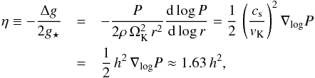 (4)where we introduced the pressure logarithmic gradient ∇log P ≡ −d(log P)/d(log r), the Keplerian velocity vK ≡ ΩKr, and the disk aspect ratio h ≡ cs/vK = H/r. The numbers are obtained from an MMSN disk with the above power law profiles for density and temperature. It follows that the motion of the disk is less than Keplerian (Weidenschilling 1977a); the gas flows at a speed equal to (1−η) vK. Also, the headwind that is faced by a big body (a.k.a. planetesimal), which moves at a Keplerian speed through the sub-Keplerian rotating gas, then reads
  (5)which, for an MMSN disk is independent of the distance r to the star.
2.2. Turbulence model
The gas has a mean-free path of  where σmol ≈ 2 × 10-15 cm2 (Chapman & Cowling 1970) is the molecular cross section. The kinematic molecular viscosity of the gas is νmol = (1/2) vthℓmfp where
  is the mean molecular thermal speed.
However, for these parameters the resulting diffusion timescales ~r2/νmol are too long to explain, for example, the measured accretion rate in T-Tauri disks. Consequently, protoplanetary disks are expected to be mildly turbulent, but still subsonic, with a turbulent eddy viscosity νt assumed to be much larger than the molecular kinematic viscosity. An often used parameterization is the alpha-viscosity model of Shakura & Sunyaev (1973):  (6)The dimensionless constant α is a disk-dependent parameter. Its value may range from a minimum of α ≈ 10-5, when the turbulence originates from the Kelvin-Helmholtz instability of a dust layer at the mid-plane, to perhaps α ≈ 0.1 for the most violent disks with a strong magneto-rotational instability (the MRI; Balbus & Hawley 1991). Generally, the saturation level of the MRI turbulence depends on the magnitude of the magnetic field that threads the disks, the level of ionization, and the amount of dust (Turner et al. 2014). Consequently, a variety of α-values can be expected (Ormel & Okuzumi 2013). But even for a weak level of turbulence – meaning, α ≪ 1 – the Reynolds number of the flow, Re = νt/νmol, is very large by virtue of the very low densities that characterize astrophysical environments. Indeed, for a MMSN density profile:
  (7)For such expected large values of the Reynolds number, one can reasonably assume that the gas flow is in a developed three-dimensional turbulent regime which can be described using Kolmogorov (1941) phenomenology. The kinetic energy is injected at a large (integral) scale L by a hydro- or magnetohydrodynamical instability. In both cases the injection mechanism is associated to the sub-Keplerian shear. The associated shear rate sets the typical turbulent large-eddy turnover time to
  (Cuzzi et al. 2001). The eddy viscosity then reads νt = L2/tL = L2 ΩK leading, together with Eq. (6), to L = α1/2H and vL ≡ L/tL = α1/2cs. Note that the assumptions of incompressibility (vL ≪ cs) and three-dimensionality (L ≪ H) of the turbulent flow in the disk are both fulfilled as long as α ≪ 1. According to Kolmogorov (1941) phenomenology, the kinetic energy cascades downscale with a constant rate
  until it reaches the smallest active scales, the Kolmogorov scale ℓKol below which it is dissipated by molecular viscosity. The typical velocity vℓ of eddies whose size ℓ lies in the inertial range ℓKol ≪ ℓ ≪ L reads vℓ ≃ (εKolℓ)1/3. The Kolmogorov length is defined as the scale where the scale-dependent Reynolds number Re(ℓ) ≡ vℓℓ/νmol is unity, so that
  and the associated timescale
  . The integral Reynolds number Re = νt/νmol gives the extension of the inertial range: L/ℓKol = Re3/4 and tL/tKol = Re1/2.
2.3. Dimensionless quantities
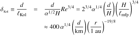
Let us now turn back to our original problem, that is the aerodynamic interactions between the disk gas flow and a solid planetesimal of size Rp, diameter d = 2Rp. There are three dimensionless quantities characterizing the system: (the numerical values below are those obtained for an MMSN disk)
-
the planetesimal Reynolds number
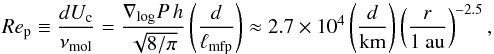 (8)which corresponds
to the strength of inertia with respect to molecular viscous forces for the gas flow
surrounding the planetesimal and characterizes how turbulent is its wake.
(8)which corresponds
to the strength of inertia with respect to molecular viscous forces for the gas flow
surrounding the planetesimal and characterizes how turbulent is its wake. -
the turbulent intensity
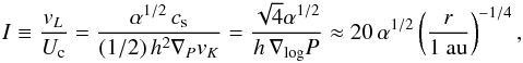 (9)which
measures how strong the turbulent velocity fluctuations are compared to the speed of
the planetesimal slip.
(9)which
measures how strong the turbulent velocity fluctuations are compared to the speed of
the planetesimal slip. -
the ratio between the planetesimal size and the Kolmogorov scale
 (10)which
measures the range of turbulent eddies that might interfere with the planetesimal
perturbation of the gas flow. It is indeed known that the flow perturbation occurs
on scales of the order of d, so that all turbulent eddies of sizes
between ℓKol and d can potentially
modify the gas flow around the spherical planetesimal.
(10)which
measures the range of turbulent eddies that might interfere with the planetesimal
perturbation of the gas flow. It is indeed known that the flow perturbation occurs
on scales of the order of d, so that all turbulent eddies of sizes
between ℓKol and d can potentially
modify the gas flow around the spherical planetesimal.
In the laminar case, Rep = 400 corresponds to a 1 km planetesimal located at ~5 au in the MMSN disk, or e.g. to a 10 km planetesimal at ~12 au.
For the turbulent case, ideally we should find parameters for which all three lines match with parameters of the numerical experiments. However, because of the ~106 mismatch between the Reynolds number in the disk and the maximum one that can be attained by present-day numerical simulations, this is not yet possible. We come back to this issue when applying the results of numerical models to real disk conditions.
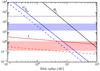 |
Fig. 1 Turbulent disk parameters: planetesimal Reynolds number Rep (black), dimensionless turbulent intensity I (red), and planetesimal to Kolmogorov scale d/ℓKol (blue) for a MMSN disk model, disk turbulent parameters α = 10-4 (dashed) and α = 10-2 (solid) and planetesimal diameter d = 1 km. The blue and black line thus scale up and down with the planetesimal size. The shaded regions are covered by the numerical experiments (see Table 1). |
3. Numerical model
3.1. Gas flow
We focus on the collision rate of a stream of dust particles with one spherical planetesimal. To study this situation we perform 3D direct numerical simulations (DNS) of a hydrodynamic flow around a spherical object with a no-slip boundary conditions at its surface. The overall method consists in a combination of a standard pseudo-Fourier-spectral solver with a penalty method that is explained in this section.
We integrate the incompressible Navier-Stokes equations 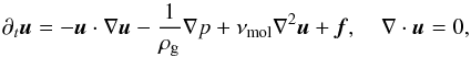 (11)for the gas velocity u, where ρg is the gas density, νmol its kinematic molecular viscosity and f a force. The latter maintains a uniform inflow speed and an eventually ambient turbulent flow. Its form is described later. The pseudo-Fourier-spectral approach consists in computing spatial derivatives in Fourier-space and convolutions arising from the non-linear terms in real space. A Fast-Fourier transform is used to switch between the two spaces. We use the P3DFFT library (see Pekurovsky 2012) that is very efficient on massive parallel computers.
The Navier–Stokes equation is integrated in the reference frame of the planetesimal. The spatial average of the velocity field is thus fixed and given by the planetesimal speed Uc relative to the gas. Equation (11) is associated with a no-slip boundary condition at the surface of the planetesimal, which is assimilated to a spherical object at rest whose diameter is denoted by d and its center by XS. We thus have  (12)Numerically, this no-slip condition is enforced by an immersed boundary technique (IBM). The latter technique was first used to simulate the blood in flow in the context of a human heart by Peskin (1972). Today, a variety of different approaches exists (Mittal & Iaccarino 2005). Generally speaking, IBM consists in solving fluid equations in domains with complex boundary conditions such as moving heart valves on Cartesian grids. As such boundaries are generally not grid conform, their effect on the flow has to be modeled. For our problem of a spherical obstacle at rest, the idea consists in defining the velocity field in the full domain enforcing a vanishing velocity in the entire object, that is for all x such that | x − XS | ≤ d/ 2. The Navier-Stokes Eq. (11) then has to be modified by introducing in its right-hand side a penalty force fb(x,t), which acts as a Lagrange multiplier associated to the constraint defined by the boundary condition (12). The full problem (11)−(12) can then be rewritten as
  (13)where L(u) denotes the right hand side of (11). In order to compute fb we make use of a direct forcing method introduced by Fadlun et al. (2000) where we directly impose the planetesimal velocity to the grid using the technique of a pressure predictor and an improved modeling of the spherical inclusion. Benchmarks (see Homann et al. 2013) of this method for a fixed sphere show good agreement with existing data. This method has also been used for the study of moving neutrally buoyant particles in homogeneous isotropic turbulence in Homann & Bec (2010) and Cisse et al. (2013). A similar IBM has been used by Uhlmann (2005) together with a second order finite-difference Navier-Stokes solver to simulate turbulent suspensions involving many particles.
3.2. Dust particles
Dust particles are modeled by spherical inertial particles with a radius a much smaller than the smallest scales of the flow, so that they can be approximated by point particles. Further, we assume that these particles move sufficiently slow with respect to the gas and that their mass density ρp is much higher than the gas density ρg. With these assumptions the dominant hydrodynamic force exerted by the gas is a drag force, which is proportional to the velocity difference between the particle and the gas flow (see Maxey & Riley 1983; Gatignol 1983) ![Mathematical equation: \begin{equation} \ddot{\bm X} = \frac{1}{\taus}\! \left[\bm u(\bm X\!,t) \!-\! \dot{\bm X} \right] \label{eq:particles} \end{equation}](/articles/aa/full_html/2016/05/aa27344-15/aa27344-15-eq89.png) (14)where the dots stand for time derivatives. ts is called the response (or stopping) time and is a measure of particle inertia. It is the relaxation time of the particle velocity to that of the gas (see Guillot et al. 2014, for a description of how the particle size relates to the stopping time). Finally, we also assume that the particles are sufficiently diluted to neglect any interaction among them and any back-reaction on the flow.
(14)where the dots stand for time derivatives. ts is called the response (or stopping) time and is a measure of particle inertia. It is the relaxation time of the particle velocity to that of the gas (see Guillot et al. 2014, for a description of how the particle size relates to the stopping time). Finally, we also assume that the particles are sufficiently diluted to neglect any interaction among them and any back-reaction on the flow.
 |
Fig. 2 Instantaneous streamlines of the gas flow (entering from the right with a speed Uc) around a planetesimal with Rep = 400 and dust particles (St = 0.8) for I = 0 (laminar, δKol = 0), I = 0.29 (moderately turbulent, δKol = 25), and I = 1.18 (strongly turbulent, , δKol = 70) from top to bottom. |
Usually, particle inertia is quantified in terms of the Stokes number St = ts/tc defined by non-dimensionalizing their response time by a characteristic time scale tc of the carrier flow. The present problem involves different relevant time scales. Td = d/Uc, the time it takes a dust particle to pass the planetesimal, tL, the turbulent large-eddy turn-over time and tKol, the turbulent dissipation time scale. If not otherwise specified, we use tc = Td as this time scale rules the collision efficiency in the laminar regime: particles with small St are closely coupled to the flow and are swept around the obstacle. Large St particles preferentially collide with it1.
In studies concerned with the small-scale dynamics of inertial particles one usually uses tc = tKol (Bec et al. 2006) and we denote the associated Stokes number StKol.
3.3. Simulation setup
We performed simulations of a planetesimal moving through a uniform and different turbulent flows. The physical situation is illustrated in Fig. 2 where the planetesimal, together with dust particles are shown in a small slice. These are snapshots taken from our three-dimensional simulations. The planetesimal experiences a headwind speed Uc from the right that is advecting the dust particles. The upper panel is taken from a simulation with a uniform inflow while the two others include turbulence with two different intensities. Dust particles that have collided with the planetesimal are missing downstream, resulting in an empty region behind the planetesimal that is clearly visible for the laminar flow, but much less for the turbulent cases.
These figures show important differences between laminar and turbulent gas flows. The spatial distribution of the dust as well as its local velocity strongly depend on the carrier flow type. Note that while St = 0.8 for all cases shown in Fig. 2, StKol = 1.25 for I = 0.29 and StKol = 9.8 for I = 1.18 so that the clustering properties of the particles change from one value of I to the other.
The runs involving a turbulent flow are set up in the following way (see Table 2 for parameters and definitions). An initially smooth large scale flow is integrated according to (11) without any forcing f. Once a turbulent flow has developed (after approx. 1−2 tL) the velocity field is forced by keeping constant the energy content of the two lowest wave number shells (1 ≤ k ≤ 2) in Fourier space. This leads to a statistically stationary turbulent flow to which the planetesimal is added. For this, the root-mean-square value vL of the velocity fluctuations is normalized to the values given in Table 2 for each simulation. A mean velocity of Uc in one direction is imposed by keeping constant the zero Fourier mode of the corresponding component of the velocity. The planetesimal is modeled via the mentioned immersed boundary method. The integration is continued until a statistically stationary state is reached again. At this point, inertial particles are seeded at a constant rate into the flow in a plane sufficiently far from the planetesimal so that they have enough time (>ts) to relax to the flow. During the simulation we remove and record all the particles that are touching the spherical planetesimal or reaching the end of the computational domain. On average the domain is filled with approximately ten million particles.
The laminar flow simulations (see Table 1 for parameters and definitions) start with a uniform flow (Uc = 1) in which the planetesimal is placed. Disturbances produced by its wake are removed at the end of the computational domain via another application of the penalty method, so that they are not re-injected upstream the planetesimal by the periodic boundary conditions. The dust particles are introduced into the flow once a (statistically) stationary state is reached.
The time integration of (11) uses a Runge-Kutta scheme of third order. The grid resolution is chosen in order to resolve all small scales of the problem: those of the spherical planetesimal boundary layer, all turbulent scales in its wake and the smallest scales of the possibly turbulent ambient flow.
All physical flow parameters are determined by three dimensionless parameters: the Reynolds number of the planetesimal Rep = Ucd/νmol, the Reynolds number of the gas Re = vLL/νmol, L being the integral scale of the ambient turbulent flow, and the turbulent large-scale intensity I = vL/Uc. The latter measuring the strength of the large-scale turbulent fluctuations compared to the mean flow velocity. In the laminar case (Re = 0, I = 0), we varied the planetesimal Reynolds number Rep from 100 to 1000. We analyze the effect of turbulent fluctuations for one specific choice of the planetesimal Reynolds number, namely Rep = 400 (turbulent wake) and vary I from 0.14 to 1.18. The corresponding flow Reynolds numbers Re (listed in Table 2) are a consequence of our particular choice of the external force. Freezing the energy content of the lowest shells in spectral space does not allow for changing L but only vL that enters in the definitions of both I and Re.
The particle dynamics is characterized by the Stokes number St. In all simulations we consider streams of heavy dust particles with response times ts in between 0.04 and 81.92, corresponding to Stokes numbers St in the range 0.05 ≤ St ≤ 63. The main parameters of all simulations are summarized in Tables 2 and 1.
Parameters of the turbulence simulations.
Parameters of the laminar simulations.
4. Results
4.1. Laminar settings
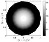 |
Fig. 3 Projected frontal view of the average probability density of impaction on the planetesimal for dust particles with St = 0.2. White: many collisions; black: no collisions. |
In a uniform gas flow all dust particles have the same velocity far from the planetesimal. This physical situation is fully determined by the Reynolds number of the planetesimal Rep and the Stokes number St of the dust particles. A typical flow pattern is illustrated in the upper panel of Fig. 2 where a planetesimal flies through a stream of dust particles while creating a moderately turbulent wake. If an approaching dust particle collides with the planetesimal or not is only determined by its Stokes number and impact parameter. Without the hydrodynamic flow that deflects dust around the obstacle it would just be the impact parameter ruling the collision rate so that the hydrodynamic forces reduce the collision rate below that of the geometric cross section.
The colliding dust particles preferentially hit the planetesimal on the axis of symmetry with a decreasing probability to its edge. Small inertial particles only touch the planetesimal in a central region leaving eventually an outer non-collisional ring (see Fig. 3). But this region already disappears for Stokes numbers around unity, so that dust collisions fill the complete front of the spherical planetesimal. In the limit of infinite St the distribution becomes uniform. Rear collisions virtually never happen (see Fig. 4) in a laminar flow that is because inertia prevents those particles that moved around the planetesimal from getting into the recirculation region of the wake. The few records observed might be numerical noise.
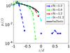 |
Fig. 4 Probability density function of the stream-wise position z at which colliding particles impact the planetesimal. The center of the planetesimal is located at z = 0 and separates its front (negative z) from its back (positive z). The “ballistic” curve refers to straight dust trajectories that do not feel any hydrodynamic forces. |
A central quantity of the accretion problem is the collision efficiency (or collision rate) E(St) that is the ratio between the actual collision rate and that expected for free-streaming particles that do not feel any hydrodynamic force from the gas flow. The latter rate is obtained from the geometrical cross-section of the planetesimal and reads ndUcπd2/ 4, where nd designates the number density of dust particles. We use the following notation: E0 denotes the uniform gas flow case that we are going to analyze in this section and EI denotes the turbulent case parameterized by the turbulent intensity I that is discussed in the following section. The efficiency E0 is a monotonously increasing function of the dust particle Stokes number St that asymptotically reaches unity for particles with very large inertia (see Fig. 5). The higher is Rep the more probable are collisions, especially at small St. In this low inertia limit, E0 sharply drops for all Rep. The reason for this is the well established existence of a critical Stokes number Stc below which no collisions occur at all (Taylor 1940).
Indeed, in the case of an inviscid Euler flow (zero viscosity, Rep = ∞) it can be shown that E0 drops to zero for small but finite  (Ingham et al. 1990). The viscous boundary layer of a finite Rep planetesimal that shrinks as ~
 reduces the collision probability and increases Stc. For the limiting case of a Stokes flow Michael & Norey (1970) computed numerically a critical Stokes number of 0.605.
Slinn (1974, 1976, 1983) proposed a fitting function of the collision rate of the form ![Mathematical equation: \begin{equation} \label{eq:slinn} \begin{cases} E_0^{\text{Slinn}}(\St,\Rep)=\left(\frac{\displaystyle{\St-\St^{\text{Slinn}}_{\rm c}}}{\displaystyle{\St-\St^{\text{Slinn}}_{\rm c}+2/3}} \right)^{3/2} \\[1em] \St^{\text{Slinn}}_{\rm c}(\Rep)= \frac{\displaystyle{0.6+(1/24)\, \log(1+\Rep/2)}}{\displaystyle{1+\log(1+\Rep/2)}}\cdot \end{cases} \end{equation}](/articles/aa/full_html/2016/05/aa27344-15/aa27344-15-eq169.png) (15)
(15) is thus a critical number below which the (extremely low) collision probability is determined by different physical mechanisms. These expressions appear to have been fitted empirically to both experimental and numerical data with uncertainties of order 0.1 on the determination of E0(St) (see Slinn 1974).
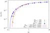 |
Fig. 5 Collision efficiency as a function of the dust particle Stokes number obtained from direct numerical simulations with uniform inflows (symbols). The lines correspond to the fitting formula (15) proposed by Slinn (1983). |
It is useful to look in more detail at the small and large St efficiencies separately. In Fig. 6 the collision efficiency is shown as a function of St − Stc and not simply as a function of St. We hence focus on the behavior of the collision probability when approaching the critical Stokes number. Stc is chosen in such a way that all curves fall on top of each other so that differences for different Reynolds numbers disappear. Our estimated Stc are close to that of Slinn (15) (see inset of Fig. 6). The case of large but finite values of Rep has also been addressed by Phillips & Kaye (1999), using matched asymptotics together with numerical simulations of the particle dynamics inside the obstacle boundary layer. They found critical Stokes numbers slightly larger than those of Slinn (15), so that our value are in between these two predictions.
E0 increases linearly at small St − Stc (see Fig. 6), that is in contradiction to Slinn’s formula (15) that predicts  . To incorporate this small-Stokes behavior we propose the fitting function
 ![Mathematical equation: \begin{equation} \label{eq:e_fit} \begin{cases} E_0(\St,\Rep)=\frac{\displaystyle{\St-\St_{\rm c}}}{\displaystyle{\St-\St_{\rm c}+2/3}} \\[1em] \St_{\rm c}(\Rep)= \frac{\displaystyle{0.6+(1/24)\, \log(1+\Rep/6)}}{\displaystyle{1+\log(1+\Rep/6)}} \end{cases} \end{equation}](/articles/aa/full_html/2016/05/aa27344-15/aa27344-15-eq175.png) (16)which is in excellent agreement with our data. Here we mention (as already remarked by Slinn) that an exponential fit of the form exp(−a/St) also works quite well for not too small St but this form does evidently not conform to a critical Stokes number.
(16)which is in excellent agreement with our data. Here we mention (as already remarked by Slinn) that an exponential fit of the form exp(−a/St) also works quite well for not too small St but this form does evidently not conform to a critical Stokes number.
We also note that Slinn (1974) had also proposed a similar fit (linear instead of with a 3/2 exponent), but opted for Eq. (15)which showed a marginal improvement to the experimental and numerical data available at the time. The uncertainties that we obtain here are much smaller and allow to discriminate against the fit from Eq. (15).
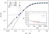 |
Fig. 6 Collision efficiency as a function of St − Stc, where Stc is the critical Stokes number below which no collision happen. fit = (St − Stc)/(St − Stc + 2/3) (Eq. (16)). The solid line indicates a linear increase. Inset: Critical Stokes number as a function of the planetesimal Reynolds number. fit = |

To study the large-Stokes number behavior in details it is useful to analyze 1 − E0(St) that measures how the free-streaming particle limit is recovered as a function of St. All curves for different Rep (see Fig. 7) fall on the top of each other and reveal a St-1 behavior at large St. Again, we observe slight deviations to Slinn’s fitting formula, while our proposed expression (16) fairly matches the data.
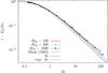 |
Fig. 7 Collision efficiency deficit 1 − E0(St) as a function of St for different planetesimal Reynolds numbers and the various fitting formula, as labeled. |
4.2. Turbulent settings
One can expect that turbulent velocity fluctuations of the gas, resulting in dust velocity fluctuations, alter the collision statistics of dust and planetesimals. An analysis of these changes is the subject of this section.
The turbulent accretion problem involves more parameters than the laminar problem presented in the previous section. It is determined by four dimensionless parameters. The planetesimal and dust properties are of course still described by the Reynolds number Rep and the dust Stokes number St, but turbulence adds two additional dimensionless parameters specifying the ambient turbulent flow. They are the gas Reynolds number Re = vLL/νmol and the turbulent intensity I = vL/Uc that compares the amplitude of turbulent fluctuations with the mean velocity of the gas.
In this work, we explicitly vary St and the turbulent intensity I and fix the planetesimal Reynolds number to Rep = 400 (weakly turbulent wake) in order to limit computational costs. The gas Reynolds number Re is implicitly varied as it is coupled to I due to our specific forcing scheme that prescribes L to approximately half of the domain size.
The physical situation for two different turbulent intensities is illustrated in the mid and bottom panel of Fig. 2. Dust particles are in these cases advected by a chaotic and irregular flow possessing coherent structures, i.e. structures eventually persisting for a long time. This has two important implications: first, the velocity of dust is fluctuating spatially and temporally (see Figs. 2b and c) and in turn (as we study in details below) modifies the collision statistics. Second, from studies of hydrodynamic turbulence it is known that inertial particles tend to escape from coherent rotating regions of the flow and tend to cluster in straining regions (Squires & Eaton 1991). These agglomerations are called preferential concentrations Shaw (2003), Balachandar & Eaton (2010). However, we expect that these concentrations play a negligible role for the present study in which we are concerned with averaged accretion quantities such as the collision efficiency. The reason is that the temporally averaged dust concentration in the ambient flow is approximately the same as in the laminar case (not shown) so that particle density fluctuations average out.
4.2.1. Collision efficiency
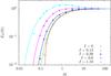 |
Fig. 8 Collision efficiencies for several turbulent intensities I = vL/Uc and Rep = 400. The I = 0 curve is the same as in Fig. 5. Solid lines: fits of the function EI(St) = exp(−a(I) /St) (1 + b(I) St/ (1 + St2)) with: a = 0.49, b = −0.095 for I = 0.14; a = 0.38, b = −0.04 for I = 0.29; a = 0.21, b = 0.31 for I = 0.60; a = 0.085, b = 1.08 for I = 1.18. |
Turbulent fluctuations significantly increase the collision probability. Figure 8 shows the collision efficiency EI for various I. One observes that higher is the turbulent intensity I, more collisions happen. This increase is the strongest at small St and disappears asymptotically at large St. As is discussed later, the collision efficiency around St ≈ 1 remarkably exceeds unity.
For the smallest Stokes numbers and the largest turbulent intensity we observe more than one hundred times more collisions than in the reference laminar flow. This relative increase ΔE(St,I) = EI/E0 − 1 of the turbulent efficiency compared with the laminar one is shown in Fig. 9. It is represented as a function of St − Stc that is the distance from the critical Stokes number Stc as ΔE diverges when St → Stc. The large values of ΔE at small St decreases as a power law with an exponent close to −1. The dependence of ΔE on I is nearly quadratic. Indeed, the different curves almost fall on the top of each other when normalized by I1.7 as can be seen from the inset of Fig. 9.
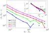 |
Fig. 9 Relative increase of the collision efficiency for several turbulent intensities as a function of the distance from the critical Stokes number of the laminar case. |
Turbulent collision efficiencies (compare Fig. 8) are well fitted by the function  (17)containing two parameters a and b. The dependence of these parameters on the turbulent intensity is shown in Fig. 10 together with simple fitting formulas. The parameter a is decreasing roughly exponentially as a function of I. b is close to zero for small intensities and strongly increasing starting from I ≈ 0.4.
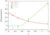 |
Fig. 10 Dependence of the fitting parameter a and b on the turbulent intensity I, for Rep = 400. fa = 0.65 exp(−1.8 I) is fitting function for the parameter a, |

In the small Stokes number limit, the turbulent collision efficiency displays a clear exponential falloff (see Fig. 11) indicating that the critical Stokes number disappears when turbulence influences the dust motion. Additionally, curves for different I fall approximately on top of each other once shown as a function of StL = tsvL/L. It is thus a turbulent time scale, namely the large-eddy turn-over time, that replaces the advection time d/Uc relevant for the laminar problem.
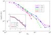 |
Fig. 11 Logarithm of collision efficiencies showing the exponential character at small StL = tsvL/L. Inset: probability density function (PDF) of stream-wise velocity gradient normalized to standard deviation within the boundary layer. |
There are different ways in which turbulence enhances the collision probability. Fluctuations of the headwind speed mix collision efficiencies for different I and St and allow for collisions of dust particles beyond the critical Stokes number Stc. In turbulent gas flows, the dust heads onto the planetesimal with a fluctuating velocity. The probability distribution of the headwind is given by the one-point turbulent velocity distribution that is known to be close to a Gaussian. For the present problem, its standard deviation is given by the turbulent intensity I. These headwind variations lead to a fluctuating planetesimal Reynolds number and to fluctuating dust Stokes numbers. Especially close to the laminar value Stc this results in higher collision probabilities and an absence of a critical Stokes number. Another consequence of a variable headwind are fluctuations of the stream-wise velocity gradient σ in the upstream boundary layer of the planetesimal. They modify the local Stokes number that can be defined by St = tsσ. The probability for a collision of a dust particle with stopping time ts is then P(St>Stc) = P(σ>Stc/ts), and thus relates to the probability of observing a large velocity gradient at the particle surface. The probability density function (PDF) of σ shown in the inset of Fig. 11. The tails are close to exponential, although we cannot rule out stretched exponential tails as observed in homogeneous isotropic turbulence. Exponential tails mean P(σ>Stc/ts) ~ exp(−CStc/ts) which is consistent with the formally observed exponential fall off of EI(St) at small values of St.
Another mechanism to increase the collision probability relates to turbulent diffusion. This enhances the mobility of dust and increases its flux onto the planetesimal. As a simplified gedankenexperiment one can think of a sphere moving in a sinusoidal velocity field representing the large-scale turbulent fluctuations. Let us assume (in the reference frame of the sphere) a velocity of the form u = Ucex + I sin(2π/tL,t) ey. The volume swept by the sphere is evidently larger in the turbulent case (I> 0) than in the laminar (I = 0). According to inertia, dust particles are more or less coupled to the gas which makes the swept volume additionally depending on St. Small St particles stick to the gas trajectories so their swept volumes equal. This effect can explain the observation of collision efficiencies exceeding unity in turbulent flows. For large St, particles move ballistically so that they only sweep through the laminar (I = 0) volume.
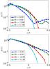 |
Fig. 12 Probability of collisions as a function of the stream-wise position for I = 0.29 (top) and I = 0.6 (bottom). |
We conclude this section with a study of the spatial distribution of dust impacts on the surface of a planetesimal in a turbulent disk. In Fig. 4 we saw that dust collisions preferentially happen close to the stagnation point of the flow in a quiescent disk. This is still true when turbulent fluctuation agitate the dust (see Fig. 12). But the added randomness leads to a homogenization of the impact position. The larger is I the more the collisions fill the entire planetesimal surface. And especially for small St particles, backward collision become frequent.
4.2.2. Impact velocity
The relative velocity of dust and a planetesimal at impact is crucial for the dust accretion problem as it determines, together with the angle of impact, the outcome of a collision. Low collision speeds lead to sticking of dust on the target surface, while high speeds lead to bouncing, fragmentation with mass transfer or erosion (e.g., Blum & Wurm 2008; Windmark et al. 2012).
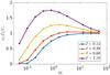 |
Fig. 13 Mean dust velocity at impact on the planetesimal surface for Re = 400. |
In laminar disks the mean impact speed of small-size dust (with a stopping time smaller than the orbital period) is a monotonously increasing function of inertia (Weidenschilling 1977a). Dust particles with inertia close to the critical Stokes number only slightly touch the planetesimal surface while large St particles collide with the full headwind speed. Dust particles in turbulent disks experience gas velocity fluctuations and in turn drag variations. They follow preferentially turbulent structures with characteristic time-scales that equal their response time. This coupling of inertial particles is known to create non-trivial phenomena such as the mentioned small-scale preferential concentrations that are the most effective for StKol = ts/tKol ≈ 0.6 particles (Reade & Collins 2000; Bec et al. 2006).
We observe such a eddy-dust coupling also for the collision velocity vc (the norm of the dust velocity vector at impact) of dust particles with a planetesimal (see Fig. 13). Asymptotically, small-St dust (small in the sense of particles with a small collision efficiency) still only mildly touches the surface, while large-St dust collides with the speed of the headwind. However, at intermediate values of St, turbulent velocity fluctuations lead to an increase of the collision speed that even exceeds the headwind speed. For the highest turbulent intensity that is studied here (I = 1.18), the average impact speed is approximately 75% higher than the mean headwind speed. We remark that once particle inertia is measured in terms of the characteristic time scale of turbulent structures of size d (planetesimal diameter) td = tL (d/L)2/3 (td = 4.4,2.1,1.1 for I = 0.29,0.6,1.18) all maxima of the curves (located at St ≈ 3.2,1.6,0.8) in Fig. 13 align at St = ts/td ≈ 0.6. Turbulent eddies of the size of the planetesimal are thus responsible for this increase of the impact velocity.
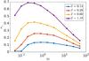 |
Fig. 14 Standard deviation of the impact speed for Re = 400 and several turbulent intensities. |
To estimate the broadness of the velocity distributions we measured in Fig. 14 their standard deviation. Here, the St ≈ 1 peak is even more important than for the mean impact speed. For a St = 0.4 dust particle in a I = 1.18 headwind, the velocity distribution is up to six times broader than in a non-turbulent disk.
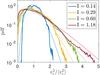 |
Fig. 15 Probability density function of the impact velocity normal to the planetesimal surface for St = 0.8 and several turbulent intensities as labeled. The bold lines correspond to measurements from numerical simulations, while the thin lines refer to the non-central chi-squared prediction (see text). |
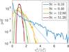 |
Fig. 16 Probability density function of the surface normal impact velocity for I = 0.29 and several Stokes numbers as labeled. As in Fig. 15, the bold lines correspond to numerical simulations and the thin lines refer to the non-central chi-squared prediction. |
The impact speed has, besides its average value and standard deviation, a probability distribution that varies with both I and St. It reveals that high-impact speeds of the order of several times the headwind speed are quite probable. For a fixed value of St the distribution becomes monotonously broader with increasing I (see Fig. 15). The numerical data is there compared to the non-central chi-squared distribution that would be obtained if vc were the norm of a three-dimensional random Gaussian vector with prescribed mean and variance. Up to statistical accuracy, it seems from Fig. 15 that such an approach gives a rather good description of actual fluctuations of the impact velocity. This approximation is however valid only if the Stokes number St is sufficiently large. Figure 16 indeed represents the same distributions for a fixed value of I at varying St. One observes deviations from the chi-squared prediction in both tails at the smallest value of the Stokes number. It seems nevertheless that the distribution still belongs to the same family and can be approximated by a chi-squared distribution with a smaller number of degrees of freedom. Everything happens as at small St, the dust velocity fluctuations with respect to the planetesimal were constrained in a space with dimension less than three.
The outcome of a collision also depends on the angle of impact. Figure 17 shows the average collision angle  with respect to the surface normal direction n. Small St dust preferentially touches the planetesimal with an mean impact angle close to 90°. High inertia dust heads straight onto the planetesimal and experiences an average impact angle of 45°. Turbulent fluctuations randomize the impact angle and favor this way to the same mean angle of
  .
.
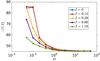 |
Fig. 17 Average angle of impact |

5. Astrophysical application
5.1. Linear cross section
We apply these results to realistic disk conditions. In order to study filtering of dust by planetesimals, Guillot et al. (2014) had applied the results of numerical simulations by Sekiya & Takeda (2003) for a laminar disk and a fixed planetesimal Reynolds number Rep = 50. Our simulations in the laminar case cover a range of Rep from 100 to 1000. As seen in Fig. 1 and Eq. (8), this corresponds to planetesimals with diameters between 4 m and 40 m at 1 au and between 1 km and 12 km at 10 au. Since the outcome of the simulations is only weakly dependent on Rep (the critical Stokes number is a function of log (1 + Rep/ 2) – see Eq. (16)), we expect to be able to extrapolate the results outside this range.
In most cases however, turbulence is expected to be important. Our simulations in the turbulent case have been calculated for various intensities of the turbulence I, but a fixed planetesimal Reynolds number Rep = 400. However, when turbulence becomes important, we expect the results to become very weakly dependent on Rep. This is for two reasons: First as seen in Fig. 2, for values of I approaching unity, the flow around planetesimals is perturbed very significantly and becomes controlled by the turbulence of the disk instead of by the planetesimal properties. Second, turbulence perturbs the boundary layer around the planetesimal independently of its properties to offer new possibilities for dust particles to impact.
But for small planetesimals and/or low turbulent intensity, the planetesimal size can become smaller than the Kolmogorov scale, i.e., the minimum scale for turbulent eddies. In that case, the planetesimals experience a headwind of variable intensity and direction. It is expected that, in the limit of d/ℓKol ≪ 1, the situation becomes similar to the laminar case, but with a headwind that is increased by  . We write
 ![Mathematical equation: \begin{equation} \label{eq:fhydro} f_{\rm hydro}= \begin{cases} \left[E_0(\St^*,\Rep)\right]^{1/2} & \quad {\rm if}\quad \delta_\mathrm{Kol}=d/\ell_{\rm Kol}<1\\ \left[E_I(\St)\right]^{1/2} & \quad \mbox{otherwise} \end{cases} \end{equation}](/articles/aa/full_html/2016/05/aa27344-15/aa27344-15-eq238.png) (18)where fhydro is the collision efficiency as defined by Guillot et al. (2014),
(18)where fhydro is the collision efficiency as defined by Guillot et al. (2014),  .and E0 and EI the fitting formula (16) and (17). With this definition, 2Rpfhydro is the planetesimal linear collisional cross section and
  its surface collisional cross section. Thus, for a planetesimal smaller than the smallest turbulent eddy, the flow is considered laminar, but we account with the use of St∗ for a flow velocity that is slightly higher on average. On the other hand, when the planetesimal is larger than the Kolmogorov scale, we use the results of the simulations in the turbulent case directly.
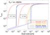 |
Fig. 18 Value of the factor fhydro (see Eq. (18)) indicative of a reduction of the linear cross section of planetesimals resulting from hydrodynamical effects as a function of dust particle size, for a planetesimal of 1 km radius in an MMSN disk, at an orbital distance of 7.1 au (plain) and 1 au (dashed) and for various levels of turbulence (as labeled). The results are compared to the one obtained by Guillot et al. (2014) which is independent of turbulence amplitude. For the 7.1 au case (which corresponds to Rep = 400 as in the previous hydrodynamical calculations), the lines corresponding to α = 10-4 and 10-6 are hidden behind the laminar case (see text). |
Figure 18 illustrates how the factor fhydro varies as a function of particle size in an MMSN disk for a 1 km-radius planetesimal either at 7.1 au or at 1 au. The first case corresponds to a planetesimal Reynolds number Rep = 400 equal to the one used in the hydrodynamical simulations with turbulence. The second case corresponds to a much higher Reynolds number Rep = 5.4 × 10⁴ outside the range of our simulations.
In all cases, particles which are larger than a critical value (i.e., with a Stokes number higher than unity) are accreted with a cross-section approximately equal to the geometric one (i.e., fhydro ≈ 1). In laminar disks or when turbulence is small, the cross section drops for small particles such that St< 1. If turbulence is large enough, this drop occurs at even smaller sizes, with an offset that corresponds to one to two orders of magnitude for the case with α = 10-2.
The comparison of the laminar Rep = 400 cases shows a relatively good agreement between our work and the previous results of Guillot et al. (2014) who used results from Sekiya & Takeda (2003) for a fixed planetesimal Reynolds number of 50. When turbulence is added, it is worth noticing that while the case with α = 10-2 stands out and allows much smaller particles to collide, the cases with α = 10-4 and 10-6 are almost indistinguishable from the laminar case. This is a direct consequence from the fact that δKol< 1 for these: the smallest turbulent cell is expected to be larger than the planetesimal size which implies that we switch to the laminar case in Eq. (18). Our approach is thus discontinuous in α, but resolving this issue would require dedicated simulations beyond the scope of the present work.
At high Reynolds number (i.e., the 1 au case in Fig. 18), the Kolmogorov parameter δKol is generally high which implies a nearly continuous behavior from high to low values of α. A small issue seen for low values of the viscosity and dust sizes corresponding to Stokes number close to unity is that the value of fhydro for a disk with low turbulence (e.g., α = 10-6) can become smaller than the laminar value, which according to our simulations is unlikely. Clearly, this is a consequence of the fact that our expressions have been derived for a relatively low planetesimal Reynolds number and are applied very far from that value. Again, dedicated simulations would be needed, but may be out of reach with present-day computing power.
5.2. Collision probabilities in disks
We now examine the consequences for collisions of dust grains with planetesimals with the same approach as Guillot et al. (2014).In protoplanetary disks, collisions between drifting dust particles and planetesimals occur with a probability  that is a function of the planetesimal cross section, the scale height of the dust disk hd and of the drift velocity of the dust particles. The latter depends on orbital distance r, orbital (Keplerian) frequency Ω and stopping time ts. In the limit that gravitational effects and gas drift may be neglected and for circular orbits, this probability can be shown to write (Guillot et al. 2014):
  (19)where fhydro accounts for hydrodynamical effects discussed previously (the purely geometrical limit is recovered for fhydro = 1).
In reality, gravity becomes important both for median to large planetesimals (kilometer size and more) and for large grains (above meter size) and seriously complicates the picture. Several interaction regimes may be defined as follows (see Ormel & Klahr 2010; Guillot et al. 2014):
-
The geometric regime, corresponds to the most simple case in which drag, hydrodynamical and gravity effects may be neglected.
-
We define the hydrodynamical regime as an extension of this regime at small dust sizes when we must account for the deflection of dust grains around planetesimals.
-
The Safronov regime corresponds to the case when large “dust” (effectively, boulders) which are very weakly affected by gas drag migrate inward so slowly that they feel a gravitational focusing by the planetesimal which increases the collision probability.
-
In the three-body regime, the gravity fields of the planetesimal and that of the central star must be taken into account.
-
The settling regime corresponds to the case when gravitational acceleration from the planetesimal and gas drag on the dust particles lead to an enhanced capture probability.
Accounting for the complexity of the problem we thus calculate the collision probability between dust and planetesimals, , from Eq. (43) of Guillot et al. (2014), assuming monodisperse size distributions2, but including fhydro from Eq. (18). In doing so, we also adopt an important modification stemming from the work of Johansen et al. (2015) and Visser & Ormel (2016): Instead of limiting the extent of the settling regime to when the capture radius is larger than the physical size of the planetesimal as in Guillot et al. (2014), we instead look for solutions of the settling regime equations outside of this range and adopt for the collision probability the maximum of the probabilities obtained in the settling and geometric+hydro regimes. This is important in regions where fhydro is extremely low but gravity and gas drag can still affect the trajectories of the dust particles.
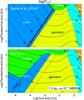 |
Fig. 19 Contours of the collision probability |
Figure 19 shows how varies with dust and planetesimal size for a fixed orbital distance of 1 au. We focus on planetesimals smaller than 100 km and down to 10 m with the caveat that for planetesimals smaller than about 1 km, gas drag should be included. The top panel shows the previous results from Guillot et al. (2014), which correspond to the case of a laminar flow and no extension of the settling regime. The bottom panel shows the results for a turbulent flow with full account for gravity effects even for low-planetesimal sizes.
The comparison between the top and bottom panels of Fig. 19 shows that even a weak planetesimal gravity effectively limits the decrease of the collision probabilities in the extended settling regime for dust smaller than ~100μm and planetesimals between one and 100 km. The inclusion of turbulence effects alsoshifts the hydrodynamic regime to smaller dust sizes. The shift is about one order of magnitude for all planetesimal sizes considered when comparing the results for α = 10-2 to those for a laminar disk. Particles of 0.1 mm can hence be accreted relatively efficiently by planetesimals for all the sizes considered. However, smaller particles still end in the hydrodynamical regime with a strongly reduced collision efficiency. For example micron-sized dust particles are very inefficiently captured by planetesimals larger than a few kilometers in size.
5.3. The inefficient capture of small dust grains
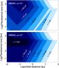 |
Fig. 20 Regions in which the collection of dust grains becomes very inefficient (defined as a collision cross section lower than 1% of the geometric one – see text) as a function of orbital distance and planetesimal radius for various dust sizes (labeled) and for two values of the turbulence: α = 10-2 (top panel) and α = 10-4 (bottom panel). Large particles are collected relatively efficiently everywhere except in the innermost regions of the disk where the gas density is assumed to be high. Small particles are inefficiently collected everywhere except at the largest orbital distances, at least in the case of a disk characterized by the MMSN gas density distribution. |
We now turn to the examination of how (in)efficiently individual small dust grains may have been collected by planetesimals as a function of their sizes and orbital distance. A full model would require studying the size distribution of dust and planetesimals and is beyond the scope of the present paper. However, we can identify the parameter space for which this collection of dust is inefficient by identifying when the collision cross section becomes smaller than 1% of the geometrical one (i.e., corresponding to fhydro< 0.1 in the limit when gravity effects are not important). Because the drop in collision probability in the hydro region of Fig. 19 is quite abrupt, we expect that if dust is indeed collected individually by planetesimals, this process should leave its imprint on the size distribution of individual grains in meteorites.
Figure 20 identifies these regions as a function of orbital distance and planetesimal size, either in the case of a high turbulence level (top panel) or a low turbulence level (bottom panel). In both cases, the collection of very small particles (nanometer sizes) is found to be very inefficient, at least inside of 10 au. Dust particles of progressively larger sizes can be collected up to shorter orbital distances, but the efficiency then strongly depends on the turbulence level.
For 1 mm particles (corresponding to a typical size of chondrules), we do not see in Fig. 20 a region of strongly inefficient collection when turbulence is high (α = 10-2), but for α = 10-4, these particles avoid collisions with planetesimals between about 0.3 and 30 km within a fraction of an au. One-micron particles are collected inefficiently inside a region extending from about 0.1 to 3 au depending on planetesimal size for α = 10-2, but this region extends from 0.8 to 6 au for α = 10-4. Smaller particles can collide with planetesimals only at larger orbital distances, when the gas density has decreased and the stopping time increased for a given particle size.
A larger turbulence level can therefore allow collisions of small-size particles which would otherwise be avoided due to the hydrodynamical flow around the planetesimals. However, this is also balanced by the fact that higher turbulence means a thicker dust subdisk which lowers the collision probability (see Guillot et al. 2014). Due to the form of Eq. (18), the effect of turbulence becomes weaker at large orbital distances, when the size of the smallest turbulent eddies becomes larger than the planetesimals. This thus explains why the contour lines for very small dust particles are identical for the α = 10-2 and α = 10-4 cases.
The change in behavior of the contour plots for α = 10-2, dust sizes between 1 μm and 1 mm and orbital distances from 0.05 to 0.3 au is due to a change in drag behavior for these particles: at short orbital distances, the gas density is so high that they are in the Stokes regimes and they switch to an Epstein drag beyond about 1 au.
For the planetesimal sizes considered, particles smaller than about 10 nm have a collision probability that is independent of alpha. This is because collisions can occur only in the outer disk where δKol< 1, i.e., the smallest Kolmogorov scale is still larger than the planetesimals considered.
Small particles such as the presolar grains present in meteorites, which can have sizes of only a few nanometers (e.g., Clayton & Nittler 2004) must have either collided with planetesimals far out in the disk or be incorporated into larger grains which would have themselves collided with planetesimals (e.g., Ormel et al. 2008). For some of the presolar grains, given their very low abundance, it remains possible that they were incorporated directly in planetesimals, although this would have to be quantified. In any case, this should have occurred without leading to any melting or dissociation of these grains which kept their identity throughout.
6. Conclusions
We have derived the accretion probability of small particles by a planetesimal in a turbulent gas. In order to do so, we performed high-resolution hydrodynamical simulations of the flow around a spherical planetesimal of diameter d moving with a velocity Uc, assuming incompressibility. We studied both the case of a laminar flow and that of a turbulent one, the intensity of the turbulence being related to the turbulent viscosity of the disk. Dust particles of variable size were implemented in the flow to determine collision rates.
For laminar flows, we confirm that small particles with a Stokes number St< 1 (corresponding to stopping times shorter than the time to cross the planetesimal) see a significant drop in their collision rate with the planetesimal. For turbulent flows however, this drop occurs for sizes that can be significantly smaller, i.e., turbulence helps accreting dust particles with sizes up to one to two order of magnitudes smaller than for laminar disks.
We thus derived collision probabilities both in the laminar case (Eq. (16)) and in the turbulent case (Eq. (17)). These expressions, even if limited to limited to Rep = 400, can be used for a wide range of situations. We propose an approximate recipe to use either the laminar case if the planetesimal size is smaller than the Kolmogorov scale and the turbulent case otherwise (Eq. (18)).
When applied to real disks, our new expressions shift the boundary with the hydro regime – where accretion rates are greatly suppressed – to smaller sizes. For example, for α = 10-2, the upper limit dust size in the hydrodynamical regime is decreased by a factor 100 and even sub-μm size particles collide efficiently with one-kilometer planetesimals. They also show that the accretion of extremely small particles is difficult and generally requires to be done by small planetesimals (less than km size) at large orbital distances (beyond 1 au) and/or late in time, when the disk has become less massive. We believe that these results are important to interpret, among other things, the presence and characteristics of presolar grains in meteorites since these vary in size from several microns down to only a few nanometers.
In order to apply our results to protoplanetary disks, we had to approximate the effect of gravity, often by extrapolations far from the regime in which numerical experiments were conducted. Future efforts will be directed towards including the gravitational force directly in our hydrodynamical simulations.
Note that in the context of astrophysical disks, a different Stokes number is often defined from τ = tsΩK. The definition of St that is used here is denoted by τf in e.g., Sekiya & Takeda (2003) and Guillot et al. (2014).
In doing so, we correct for the fact that in Guillot et al. (2014), the 3D collision probability in the hydro mode was overestimated because it neglected the reduction in the vertical cross section, i.e.,  had been assumed instead of
  . Because this affected the hydro mode with an already very low collision probability this had negligible effect on the qualitative results.
Acknowledgments
We thank Satoshi Okuzumi, Zoe Leinhart and Rico Visser for useful discussions. Most of the simulations were done using HPC resources from GENCI-IDRIS (Grant i2011026174). Part of them were performed on the “Mésocentre de calcul SIGAMM” at the Observatoire de la Côte d’Azur. The research leading to these results has received funding from the Agence Nationale de la Recherche (Programme Blanc ANR-12-BS09-011-04).
References
- Balachandar, S., & Eaton, J. K. 2010, Ann. Rev. Fluid Mech., 42, 111 [NASA ADS] [CrossRef] [Google Scholar]
- Balbus, S. A., & Hawley, J. F. 1991, ApJ, 376, 214 [NASA ADS] [CrossRef] [Google Scholar]
- Bec, J., Biferale, L., Boffetta, G., et al. 2006, J. Fluid Mech., 550, 349 [NASA ADS] [CrossRef] [Google Scholar]
- Berthet, S., Leriche, M., Pinty, J.-P., Cuesta, J., & Pigeon, G. 2010, Atmospheric Research, 96, 325 [NASA ADS] [CrossRef] [Google Scholar]
- Blum, J., & Wurm, G. 2008, ARA&A, 46, 21 [NASA ADS] [CrossRef] [EDP Sciences] [Google Scholar]
- Chapman, S., & Cowling, T. G. 1970, The mathematical theory of non-uniform gases. an account of the kinetic theory of viscosity, thermal conduction and diffusion in gases 3nd edn. (Cambridge University Press) [Google Scholar]
- Chatterjee, S., & Tan, J. C. 2014, ApJ, 780, 53 [NASA ADS] [CrossRef] [Google Scholar]
- Chatterjee, S., & Tan, J. C. 2015, ApJ, 798, L32 [NASA ADS] [CrossRef] [Google Scholar]
- Cisse, M., Homann, H., & Bec, J. 2013, J. Fluid Mech., 735, R1 [NASA ADS] [CrossRef] [Google Scholar]
- Clayton, D. D., & Nittler, L. R. 2004, ARA&A, 42, 39 [NASA ADS] [CrossRef] [Google Scholar]
- Cuzzi, J. N., Hogan, R. C., Paque, J. M., & Dobrovolskis, A. R. 2001, ApJ, 546, 496 [NASA ADS] [CrossRef] [Google Scholar]
- Fadlun, E. A., Verzicco, R., Orlandi, P., & Mohd, J. 2000, J. Comput. Phys., 60, 35 [NASA ADS] [CrossRef] [Google Scholar]
- Gatignol, R. 1983, J. Méc. Théor. Appl., 1, 143 [Google Scholar]
- Guillot, T., Ida, S., & Ormel, C. W. 2014, A&A, 572, A72 [NASA ADS] [CrossRef] [EDP Sciences] [Google Scholar]
- Haugen, N. E. L., & Kragset, S. 2010, J. Fluid Mech., 661, 239 [NASA ADS] [CrossRef] [Google Scholar]
- Hayashi, C. 1981, Prog. Theor. Phys. Suppl., 70, 35 [NASA ADS] [CrossRef] [MathSciNet] [Google Scholar]
- Hayashi, C., Nakazawa, K., & Nakagawa, Y. 1985, in Protostars and Planets II, eds. D. Black & M. Matthews (Tucson, AZ: University of Arizona Press), 1100 [Google Scholar]
- Homann, H., & Bec, J. 2010, J. Fluid Mech., 651, 81 [NASA ADS] [CrossRef] [Google Scholar]
- Homann, H., & Bec, J. 2015, Physics of Fluids, 27, 053301 [NASA ADS] [CrossRef] [Google Scholar]
- Homann, H., Bec, J., & Grauer, R. 2013, J. Fluid Mech, 721, 155 [NASA ADS] [CrossRef] [Google Scholar]
- Hydle Rivedal, N., Granskogen Bjørnstad, A., & Haugen, N. E. L. 2011, ArXiv e-prints [arXiv:1109.1135] [Google Scholar]
- Ingham, D., Hildyard, L., & Hildyard, M. 1990, Journal of Aerosol Science, 21, 935 [CrossRef] [Google Scholar]
- Johansen, A., Oishi, J. S., Mac Low, M.-M., et al. 2007, Nature, 448, 1022 [Google Scholar]
- Johansen, A., Klahr, H., & Henning, T. 2011, A&A, 529, A62 [NASA ADS] [CrossRef] [EDP Sciences] [Google Scholar]
- Johansen, A., Mac Low, M.-M., Lacerda, P., & Bizzarro, M. 2015, Science Advances, 1, 15109 [Google Scholar]
- Kolmogorov, A. 1941, Akademiia Nauk SSSR Doklady, 30, 301 [Google Scholar]
- Lambrechts, M., & Johansen, A. 2012, A&A, 544, A32 [Google Scholar]
- Maxey, M. R., & Riley, J. 1983, Phys. Fluids, 26, 883 [NASA ADS] [CrossRef] [Google Scholar]
- Michael, D. H., & Norey, P. W. 1970, Can. J. Phys., 48, 1607 [NASA ADS] [CrossRef] [Google Scholar]
- Mitra, D., Wettlaufer, J. S., & Brandenburg, A. 2013, ApJ, 773, 120 [NASA ADS] [CrossRef] [Google Scholar]
- Mittal, R., & Iaccarino, G. 2005, Ann. Rev. Fluid Mech., 37, 239 [NASA ADS] [CrossRef] [Google Scholar]
- Morbidelli, A., Lambrechts, M., Jacobson, S., & Bitsch, B. 2015, Icarus, 258, 418 [NASA ADS] [CrossRef] [Google Scholar]
- Nakagawa, Y., Sekiya, M., & Hayashi, C. 1986, Icarus, 67, 375 [NASA ADS] [CrossRef] [Google Scholar]
- Ormel, C., & Klahr, H. 2010, A&A, 520, A43 [NASA ADS] [CrossRef] [EDP Sciences] [Google Scholar]
- Ormel, C., & Kobayashi, H. 2012, ApJ, 747, 115 [NASA ADS] [CrossRef] [Google Scholar]
- Ormel, C. W., & Okuzumi, S. 2013, ApJ, 771, 44 [NASA ADS] [CrossRef] [Google Scholar]
- Ormel, C. W., Cuzzi, J. N., & Tielens, A. G. G. M. 2008, ApJ, 679, 1588 [NASA ADS] [CrossRef] [Google Scholar]
- Pekurovsky, D. 2012, SIAM Journal on Scientific Computing, 34, C192 [CrossRef] [Google Scholar]
- Peskin, C. S. 1972, J. Comput. Phys., 10, 252 [NASA ADS] [CrossRef] [Google Scholar]
- Phillips, C., & Kaye, S. 1999, Journal of Aerosol Science, 30, 709 [CrossRef] [Google Scholar]
- Reade, W. C., & Collins, L. R. 2000, Phys. Fluids, 12, 2530 [NASA ADS] [CrossRef] [Google Scholar]
- Safronov, V. S. 1972, Evolution of the protoplanetary cloud and formation of the earth and planets, Israel Program for Scientific Translations (Keter Publishing House) [Google Scholar]
- Sekiya, M., & Takeda, H. 2003, Earth, Planets, and Space, 55, 263 [Google Scholar]
- Shakura, N. I., & Sunyaev, R. A. 1973, A&A, 24, 337 [NASA ADS] [Google Scholar]
- Shaw, R. A. 2003, Ann. Rev. Fluid Mech., 35, 183 [NASA ADS] [CrossRef] [Google Scholar]
- Slinn, W. 1983, Atmospheric Sciences and Power Production, Chap.11 [Google Scholar]
- Slinn, W. G. N. 1974, Proc. USAEC Symposium [Google Scholar]
- Slinn, W. G. N. 1976, Geophys. Res. Lett., 3, 21 [NASA ADS] [CrossRef] [Google Scholar]
- Squires, K., & Eaton, J. 1991, Phys. Fluids A, 3, 1169 [Google Scholar]
- Taylor, G. I. 1940, Collected Works G.I. Taylor, 3, 236 [Google Scholar]
- Turner, N. J., Fromang, S., Gammie, C., et al. 2014, Protostars and Planets VI, 411 [Google Scholar]
- Uhlmann, M. 2005, J. Comput. Phys., 209, 448 [Google Scholar]
- Visser, R. G., & Ormel, C. W. 2016, A&A, 586, A66 [NASA ADS] [CrossRef] [EDP Sciences] [Google Scholar]
- Weidenschilling, S. J. 1977a, MNRAS, 180, 57 [NASA ADS] [CrossRef] [Google Scholar]
- Weidenschilling, S. J. 1977b, Ap&SS, 51, 153 [Google Scholar]
- Weidenschilling, S. J. 1984, Icarus, 60, 553 [NASA ADS] [CrossRef] [Google Scholar]
- Windmark, F., Birnstiel, T., Güttler, C., et al. 2012, A&A, 540, A73 [NASA ADS] [CrossRef] [EDP Sciences] [Google Scholar]
- Youdin, A. N., & Goodman, J. 2005, ApJ, 620, 459 [NASA ADS] [CrossRef] [Google Scholar]
Appendix A: Definition of symbols
We summarize here the symbols used in this paper and their definitions.
Symbols used in this article.
All Tables
All Figures
|
Fig. 1 Turbulent disk parameters: planetesimal Reynolds number Rep (black), dimensionless turbulent intensity I (red), and planetesimal to Kolmogorov scale d/ℓKol (blue) for a MMSN disk model, disk turbulent parameters α = 10-4 (dashed) and α = 10-2 (solid) and planetesimal diameter d = 1 km. The blue and black line thus scale up and down with the planetesimal size. The shaded regions are covered by the numerical experiments (see Table 1). |
| In the text | |
|
Fig. 2 Instantaneous streamlines of the gas flow (entering from the right with a speed Uc) around a planetesimal with Rep = 400 and dust particles (St = 0.8) for I = 0 (laminar, δKol = 0), I = 0.29 (moderately turbulent, δKol = 25), and I = 1.18 (strongly turbulent, , δKol = 70) from top to bottom. |
| In the text | |
|
Fig. 3 Projected frontal view of the average probability density of impaction on the planetesimal for dust particles with St = 0.2. White: many collisions; black: no collisions. |
| In the text | |
|
Fig. 4 Probability density function of the stream-wise position z at which colliding particles impact the planetesimal. The center of the planetesimal is located at z = 0 and separates its front (negative z) from its back (positive z). The “ballistic” curve refers to straight dust trajectories that do not feel any hydrodynamic forces. |
| In the text | |
|
Fig. 5 Collision efficiency as a function of the dust particle Stokes number obtained from direct numerical simulations with uniform inflows (symbols). The lines correspond to the fitting formula (15) proposed by Slinn (1983). |
| In the text | |
|
Fig. 6 Collision efficiency as a function of St − Stc, where Stc is the critical Stokes number below which no collision happen. fit = (St − Stc)/(St − Stc + 2/3) (Eq. (16)). The solid line indicates a linear increase. Inset: Critical Stokes number as a function of the planetesimal Reynolds number. fit = |
| In the text | |
|
Fig. 7 Collision efficiency deficit 1 − E0(St) as a function of St for different planetesimal Reynolds numbers and the various fitting formula, as labeled. |
| In the text | |
|
Fig. 8 Collision efficiencies for several turbulent intensities I = vL/Uc and Rep = 400. The I = 0 curve is the same as in Fig. 5. Solid lines: fits of the function EI(St) = exp(−a(I) /St) (1 + b(I) St/ (1 + St2)) with: a = 0.49, b = −0.095 for I = 0.14; a = 0.38, b = −0.04 for I = 0.29; a = 0.21, b = 0.31 for I = 0.60; a = 0.085, b = 1.08 for I = 1.18. |
| In the text | |
|
Fig. 9 Relative increase of the collision efficiency for several turbulent intensities as a function of the distance from the critical Stokes number of the laminar case. |
| In the text | |
|
Fig. 10 Dependence of the fitting parameter a and b on the turbulent intensity I, for Rep = 400. fa = 0.65 exp(−1.8 I) is fitting function for the parameter a, |
| In the text | |
|
Fig. 11 Logarithm of collision efficiencies showing the exponential character at small StL = tsvL/L. Inset: probability density function (PDF) of stream-wise velocity gradient normalized to standard deviation within the boundary layer. |
| In the text | |
|
Fig. 12 Probability of collisions as a function of the stream-wise position for I = 0.29 (top) and I = 0.6 (bottom). |
| In the text | |
|
Fig. 13 Mean dust velocity at impact on the planetesimal surface for Re = 400. |
| In the text | |
|
Fig. 14 Standard deviation of the impact speed for Re = 400 and several turbulent intensities. |
| In the text | |
|
Fig. 15 Probability density function of the impact velocity normal to the planetesimal surface for St = 0.8 and several turbulent intensities as labeled. The bold lines correspond to measurements from numerical simulations, while the thin lines refer to the non-central chi-squared prediction (see text). |
| In the text | |
|
Fig. 16 Probability density function of the surface normal impact velocity for I = 0.29 and several Stokes numbers as labeled. As in Fig. 15, the bold lines correspond to numerical simulations and the thin lines refer to the non-central chi-squared prediction. |
| In the text | |
|
Fig. 17 Average angle of impact |
| In the text | |
|
Fig. 18 Value of the factor fhydro (see Eq. (18)) indicative of a reduction of the linear cross section of planetesimals resulting from hydrodynamical effects as a function of dust particle size, for a planetesimal of 1 km radius in an MMSN disk, at an orbital distance of 7.1 au (plain) and 1 au (dashed) and for various levels of turbulence (as labeled). The results are compared to the one obtained by Guillot et al. (2014) which is independent of turbulence amplitude. For the 7.1 au case (which corresponds to Rep = 400 as in the previous hydrodynamical calculations), the lines corresponding to α = 10-4 and 10-6 are hidden behind the laminar case (see text). |
| In the text | |
|
Fig. 19 Contours of the collision probability |
| In the text | |
|
Fig. 20 Regions in which the collection of dust grains becomes very inefficient (defined as a collision cross section lower than 1% of the geometric one – see text) as a function of orbital distance and planetesimal radius for various dust sizes (labeled) and for two values of the turbulence: α = 10-2 (top panel) and α = 10-4 (bottom panel). Large particles are collected relatively efficiently everywhere except in the innermost regions of the disk where the gas density is assumed to be high. Small particles are inefficiently collected everywhere except at the largest orbital distances, at least in the case of a disk characterized by the MMSN gas density distribution. |
| In the text | |
Current usage metrics show cumulative count of Article Views (full-text article views including HTML views, PDF and ePub downloads, according to the available data) and Abstracts Views on Vision4Press platform.
Data correspond to usage on the plateform after 2015. The current usage metrics is available 48-96 hours after online publication and is updated daily on week days.
Initial download of the metrics may take a while.