| Issue |
A&A
Volume 588, April 2016
|
|
|---|---|---|
| Article Number | A85 | |
| Number of page(s) | 11 | |
| Section | Stellar structure and evolution | |
| DOI | https://doi.org/10.1051/0004-6361/201528038 | |
| Published online | 22 March 2016 | |
Multi-dimensional structure of accreting young stars
1
University of Exeter,
Physics and Astronomy, EX4 4,
QL Exeter,
UK
e-mail:
geroux@astro.ex.ac.uk
2
Max-Planck-Institut für Astrophysik, Karl Schwarzschild Strasse 1, 85741
Garching,
Germany
3
École Normale Supérieure de Lyon, CRAL (UMR CNRS 5574), Université
de Lyon 1, 69007
Lyon,
France
Received: 23 December 2015
Accepted: 5 February 2016
This work is the first attempt to describe the multi-dimensional structure of accreting young stars based on fully compressible time implicit multi-dimensional hydrodynamics simulations. One major motivation is to analyse the validity of accretion treatment used in previous 1D stellar evolution studies. We analyse the effect of accretion on the structure of a realistic stellar model of the young Sun. Our work is inspired by the numerical work of Kley & Lin (1996, ApJ, 461, 933) devoted to the structure of the boundary layer in accretion disks, which provides the outer boundary conditions for our simulations. We analyse the redistribution of accreted material with a range of values of specific entropy relative to the bulk specific entropy of the material in the accreting object’s convective envelope. Low specific entropy accreted material characterises the so-called cold accretion process, whereas high specific entropy is relevant to hot accretion. A primary goal is to understand whether and how accreted energy deposited onto a stellar surface is redistributed in the interior. This study focusses on the high accretion rates characteristic of FU Ori systems. We find that the highest entropy cases produce a distinctive behaviour in the mass redistribution, rms velocities, and enthalpy flux in the convective envelope. This change in behaviour is characterised by the formation of a hot layer on the surface of the accreting object, which tends to suppress convection in the envelope. We analyse the long-term effect of such a hot buffer zone on the structure and evolution of the accreting object with 1D stellar evolution calculations. We study the relevance of the assumption of redistribution of accreted energy into the stellar interior used in the literature. We compare results obtained with the latter treatment and those obtained with a more physical accretion boundary condition based on the formation of a hot surface layer suggested by present multi-dimensional simulations. One conclusion is that, for a given amount of accreted energy transferred to the accreting object, a treatment assuming accretion energy redistribution throughout the stellar interior could significantly overestimate the effects on the stellar structure and, in particular, on the resulting expansion.
Key words: accretion, accretion disks / stars: evolution / stars: formation / stars: pre-main sequence / hydrodynamics / convection
© ESO, 2016
1. Introduction
Accretion is an important process relevant to various fields in astrophysics, from star formation to the study of compact binaries and supernovae type Ia. Continuous theoretical and numerical efforts have been devoted to understanding the interaction between the inner edge of an accretion disk and the stellar surface. Analysis of this transition region is often based on boundary layer models that characterise this narrow region where the accreted matter leaving the disk decelerates to join the surface of the star, white dwarf or neutron star (see Pringle 1981, and references therein). Other approaches to studying the spread of accreted matter over the stellar surface are based on the so-called spreading layer model, following analytical models applied to neutron stars or white dwarfs (e.g. Inogamov & Sunyaev 1999; Piro & Bildsten 2004). Several authors have attacked the problem with multi-dimensional numerical methods (see e.g. Kley & Hensler 1987; Kley & Lin 1996; Balsara et al. 2009; Hertfelder et al. 2013). The numerical efforts from Kley & Hensler (1987) and Kley & Lin (1996), which were devoted to the accretion process on protostars, demonstrated the importance of meridional flow development over the surface of the accreting object, showing in the case of high accretion rates (FU Ori type stars) how matter accreted from a disk can spread over the poles and completely engulf the protostar.
Complementary to these works, there are also many studies devoted to the effect of accretion on the structure and evolution of objects, using either polytropic approaches (e.g. Hartmann et al. 1997) or simulations based on one dimensional (1D) stellar evolution codes (e.g. Mercer-Smith et al. 1984; Prialnik & Livio 1985; Shaviv & Starrfield 1988; Siess et al. 1997; Baraffe et al. 2009; Hosokawa et al. 2010). Despite many efforts, great uncertainties still remain regarding the amount of accretion luminosity imparted to the accreting object or radiated away, how the accreted material is redistributed over the stellar surface and the depth it reaches. Various treatments have been used, based either on modifications of the outer boundary conditions at the stellar surface (e.g. Mercer-Smith et al. 1984; Shaviv & Starrfield 1988; Palla & Stahler 1992; Hosokawa et al. 2010) or assuming that some amount of thermal energy released by accretion, and characterised by a part of the accretion luminosity, is added to the stellar interior (e.g. Hartmann et al. 1997; Siess et al. 1997; Baraffe et al. 2009). In the latter case, accretion is assumed to proceed through a disk with a part ϵ (≤1/2) of the gravitational potential energy going into the internal energy of the gas in the boundary layer. As material is incorporated into the star from the boundary layer, a part α of the energy of the gas is absorbed by the protostar and a part (1 − α) is radiated away. This leads to a rate where energy is added to the accreting protostar  (1)where M is the mass of the accreting protostar, Ṁ the accretion rate, and R the stellar radius. The parameter α is free and characterises the accretion process, with α = 0 for cold accretion and α> 0 for hot accretion (Baraffe et al. 2012).
The importance of understanding the effects of accretion on stellar structure and evolution was again highlighted in a series of works from one of the present authors (Baraffe et al. 2009, 2012; Baraffe & Chabrier 2010) within the context of early stages of evolution of young low mass stars and brown dwarfs. Early accretion history may affect the properties of objects (luminosity, radius, and effective temperature) in star formation regions and young clusters even after several Myr when the accretion process has ceased. This scenario can provide an explanation for a well known observed feature, namely the luminosity spread in Hertzsprung-Russel diagrams of star-forming regions and young clusters. Baraffe et al. (2012) proposed a so-called hybrid accretion scenario, wherein the amount of accretion energy absorbed by the protostar depends on the accretion rate. This hybrid scenario led to a proposed unified picture linking the observed luminosity spread in young clusters and FU Ori eruptions.
The work by Baraffe et al. could have important consequences for our understanding of star formation regions and young clusters. But the conclusions rely on a very simplistic approach to accretion in their stellar evolution calculations where the accreted material and energy are added instantaneously and uniformly throughout the stellar model. A more sophisticated model to describe the redistribution of accreted mass and energy within young stars has been developed by Siess & Forestini (1996), Siess et al. (1997). Their approach is based on earlier models by Kippenhahn & Thomas (1978), Kutter & Sparks (1987) developed for the study of accreting white dwarfs within the context of nova outburts. The basic idea is that the accreting material possesses angular momentum and its accretion onto a slowly (or non-) rotating stellar surface causes shear instabilities that induce mixing of material and transport the accreted angular momentum. The redistribution of mass, energy and angular momentum can be characterised by the same penetration function, which depends among other parameters, on the Richardson number Ri defined as the ratio of potential energy of buoyant force to kinetic energy of turbulence. The Siess et al. formalism is rather complex and it is difficult to gauge the added physical correctness achieved by this sophisticated model. Interestingly, while there have been several attempts to tackle the problem of boundary layers of accretion disks with multi-dimensional approaches, as previously mentioned, no multi-dimensional (hereafter multi-D) numerical study has ever been devoted to the effect of accretion on the structure of accreting objects.
This work is the very first attempt to describe with two dimensional (2D) hydrodynamic simulations the redistribution of accreted material and energy in accreting young stars. One motivation is to test some of the main assumptions used in the scenario developed by Baraffe et al. (2009, 2012), which heavily relies on the hypothesis of cold and hot accretion. In particular, the success of explaining various observations depends on the possibility of efficiently redistributing a given amount of the accreted energy within the stellar interior. More generally, the aim of such multi-dimensional simulations is to provide a clearer picture of the accretion process onto young stars and provide physical support to simple treatments of accretion used in stellar evolution codes for the wide range of astrophysical applications above-mentioned.
The hydrodynamical simulations were computed using our fully compressible time implicit code MUSIC (Multidimensional Stellar Implicit Code), initially developed by Viallet et al. (2011, 2013) and recently improved with the implementation of a Jacobian-free Newton-Krylov time integration method, which significantly improves the performance of the code (Viallet et al. 2016). This first numerical study devoted to accretion is inspired by the numerical work of Kley & Lin (1996) concerning the structure of the boundary layer in accretion disks and which provides the outer boundary conditions for our simulations. One of our primary goals is to understand whether and how accreted energy deposited onto a stellar surface can be redistributed in the interior. This first study focusses on high accretion rates characteristic of FU Ori systems and relevant to the Baraffe et al. (2009, 2012) analysis.
Our paper is organised as follows. In Sect. 2 we describe the stellar model used as a laboratory for our numerical experiments and the implementation of the accretion process in MUSIC. We analyse in Sect. 3 the effect of accretion on the stellar structure and in Sect. 4 the redistribution of accreted material assuming it has different values of specific entropy relative to the bulk specific entropy of the accreting object. Low specific entropy of the accreted material characterises the so-called cold accretion process whereas high specific entropy is relevant for the hot accretion case. The main findings resulting from the 2D calculations are transposed in our 1D stellar evolution code in Sect. 5 in order to understand the impact of our results on the evolution of accreting young stars. Finally, we discuss and conclude on the limitations and implications of these first multi-D results in Sect. 6.
2. Model of stellar accretion
2.1. Initial stellar model
Our main goal is to study the process of accretion on young stellar objects, which are essentially fully convective. We adopt as a stellar laboratory the young Sun model already used in Viallet et al. (2013, 2016) for the development and benchmarking of MUSIC. The main characteristics of MUSIC are briefly recalled below. It is a fully time implicit code solving the compressible hydrodynamic equations in spherical geometry using a finite volume method. Radiation transport is modelled with the diffusion approximation and realistic stellar equation of state and opacities are included. The code is continuously being developed and benchmarked and all numerical details are provided in the Viallet et al. series of papers. Thanks to the time implicit solver and the spherical coordinate system, MUSIC is particularly well suited for the description of convection in stellar interiors. A systematic study devoted to the sensitivity of convection properties to numerical treatments, including the resolution and extension of the spatial grid and the effects of boundary conditions, is presented elsewhere (Pratt et al. 2016). The young solar model was generated using the Lyon stellar evolution code (Baraffe & El Eid 1991; Chabrier & Baraffe 1997; Baraffe et al. 1998). It is a 1 M⊙ star of a few Myr, with radius R ~ 3 R⊙, effective temperature Teff ~ 4100 K and luminosity L ~ 2.3 L⊙, still contracting toward the Main-Sequence. Those properties are very similar to that of the central protostar adopted by Kley & Lin (1996). The model has developed a radiative core that covers ~40% of the stellar radius and a fully convective envelope covering the remaining 60% of the star. Note that energy generation from deuterium burning is not important for this particular model and does not need to be accounted for in the multi-D simulations.
The initial model for MUSIC is spherically symmetric with resolution in (r, θ) of 320 × 256 and uniform chemical composition and is created from the 1D model. Special attention is paid to the radial grid close to the surface. In the 1D model, the surface is defined using the Eddington approximation, with the surface corresponding to the photosphere at an optical depth τ = 2/3 and a surface temperature Tsurf equal to the effective temperature Teff (see e.g. Chabrier & Baraffe 1997). The small scale surface convection resulting from the rapidly decreasing pressure scale height near the surface of a star as well as steep surface radial gradients require a smaller radial spacing near the surface. We thus design the radial grid for the 2D simulations based on the following procedure. An initial radial spacing Δr0 at the surface of the stellar model is defined. Then, for each new radial cell, i, a new Δri = Δri − 1(1 + ϵ) is calculated until a fractional stellar radius r/R = 0.94 is reached (with r/R = 1.0 defining the surface). In the present work, we use ϵ = 0.05, yielding 64 shells in this region. Below r/R = 0.94 we use a fixed Δr such that 256 cells are evenly spaced between r/R = 0.94 and r/R = 0.2. Figure 1 shows a visualisation of the resulting grid, with a zoom of the outer geometrically decreasing radial spacing. In the angular direction we use 256 evenly spaced divisions. In the present case, we model a region covering θ = 20°−160°, with θ measured clockwise from the vertical axis.
Initially the 2D model has zero radial and tangential velocities. The radial grid extends down to the middle of the stellar radiative core. In 2D, MUSIC uses as independent variables the density ρ, the specific internal energy e, the radial velocity ur and the tangential velocity ut1. Periodic conditions in the tangential direction are used. The boundary conditions for velocities at the top and the bottom of the domain are based on reflective boundary conditions for the radial velocity and stress-free conditions for the tangential velocity (see Viallet et al. 2011). At the bottom of the domain, a constant energy flux, derived from the 1D initial model, is imposed and linear extrapolations as a function of radius in density and energy are used to set the values in the ghost cells. At the top of the domain, i.e. the surface, the energy flux is given by F = σT4, with σ the Stefan-Boltzmann constant and T the temperature of the cells in the top layer of the domain, in order to remain consistent with the 1D initial model. During the relaxation process of the initial model, the surface value of the density ρsurf is forced to be equal to that of the 1D initial model. The values of ρ and e in the ghost cells are the same as in the cells of the top layer. Note that values of density and energy in the ghost cells at the top and bottom of the domain are mainly used for higher order reconstruction of interface values. Uncertainties and limitations due to the boundary conditions used for present study are discussed in Sect. 6.
After a short time (<106 s) convection develops. The initial model requires some time to relax to a nearly steady state as indicated by the steady evolution of the total kinetic energy of the model with time. After this relaxation time, the model has a well developed convective region from a fractional radius r/R = 0.41 to the surface. For this particular initial model, the relaxation time to reach steady-state convection is ~2 × 10⁷ s, which corresponds to ~50 convective turnover timescales (see Sect. 3). Note that this relaxation time depends on the initial model, its radial extension and the boundary conditions, as analysed in a follow-up paper (Pratt et al. 2016). This relaxed model is the starting point for exploring the accretion process, i.e. the accretion boundary condition is only applied after this period of relaxation.
 |
Fig. 1 Visualisation of the computational mesh. On the right is a zoom of the near surface mesh showing the geometrically decreasing radial spacing. Note that the changes in grid-lines are a result of the rasterisation process to generate the figure and not indicative of a change in actual grid geometry. |
Summary of simulation parameters and results.
2.2. Multi-dimensional treatment of accretion
Accretion is implemented by applying a simple inflow boundary condition to the surface of the relaxed convective model. This is a very simplistic treatment which is far from treating the process of accretion with a fundamental physical approach. But this is a reasonable working hypothesis for our numerical experiments, given our first goal, which is to study with multi-D configurations the structure and evolution of accreting stars and to compare that to 1D approaches. The boundary values which must be specified in MUSIC for our accretion boundary condition are the inflow speed, vinflow, density, ρacc, and specific internal energy, eacc, of the accreted material. These values are set and held constant in the outer ghost cells of our simulation. ρacc is determined from vinflow and the mass accretion rate Ṁ such that  (2)where Aacc is the area over which the accretion boundary condition is applied.
The work by Kley & Lin (1996) is used as a guide to set the values for Aacc and vinflow. As mentioned in Sect. 1, we focus in this paper on high accretion rates and adopt Ṁ = 10-4M⊙ yr-1, which corresponds to model 2 of Kley & Lin (1996). For such high accretion rates, the Kley & Lin (1996) simulations suggest that the boundary layer covers the entire surface of the star. This picture is also consistent with other models based on the idea of a spreading layer where the infalling gas does not decelerate in the midplane of the disk but rather across the whole surface of the star (e.g. Inogamov & Sunyaev 1999). We thus assume Aacc to be equal to the surface area of the portion of the star we are modelling, i.e. Aacc = 4πR2sin(Δθ) with Δθ = 70°. As an estimate for the inflow speed we choose one tenth of the sound speed at the surface of the non-accreting model, or vinflow = 6.5 × 104 cm s-1 because Kley & Lin (1996) predict infall velocities of about this order of magnitude at the surface of the star. The above values yield an accretion boundary condition for the density of ρacc~2.7 × 10⁻⁷ g cm-3.
The final boundary condition that needs to be specified is the specific internal energy of the accreted material, eacc. Determining suitable values of eacc is a radiation hydrodynamics problem that requires a boundary (or spreading) layer model including the description of the accretion disk. This is a problem disconnected from our study and which cannot be addressed with our MUSIC code. We can thus only explore a range of values for eacc. Expectedly, if the accreted material is cold with a relatively low entropy, compared to the bulk entropy in the convective envelope, it will sink. Conversely hotter material with larger entropy will remain near the surface. With a given equation of state, the specific entropy of the material can be related to the specific energy and density of that material. The convective envelope in the young Sun is essentially isentropic with a specific entropy of s = 3.14 × 10⁹ erg K-1 g-1. We explore a range of values for eacc, so that the specific entropy of the accreted material sacc covers values 30% lower to 50% higher than the specific entropy in the convective region, with the intention that material with lower sacc will mix into the convective region, while that with higher sacc will remain at the surface.
In order to link the arbitrary variation of eacc to stellar evolution studies of accreting objects, we note that the value of eacc can directly be related to α in Eq. (1) by multiplying eacc by Ṁ to get a rate of energy accretion. The lowest value of eacc adopted in this work, equivalent to 30% lower entropy, corresponds to α ~ 0.01, and the highest eacc, equivalent to 50% higher entropy, corresponds to α ~ 0.2. This range of values for α is consistent with those adopted in Baraffe et al. (2012). Table 1 lists the various models we have computed, along with some relevant parameters and values of the simulation. We cover many cases in order to be able to find an eventual transition in the behaviour of accretion. The total simulation time for all cases is 3 × 10⁷ s. For all our simulations, except the highest accreted entropy case (case e9 in Table 1), the timestep is characterised by a CFL number between typically ~10 and ~80, which is essentially set by the radiative CFL number (see Viallet et al. 2011, for definitions). The hydrodynamic CFL number, CFLhydro, varies from ~1.5 to ~10 depending on the simulation. For the e9 case, the timestep reduces to an average CFL number ~2.5. Note that, for the sake of accuracy and to help convergency, the timestep is also constrained by a condition that limits the relative change in energy and density from one time step to the next to less than 1%. Reducing this constraint could allow larger CFL numbers.
3. Effects of accretion on the stellar structure
When the accretion boundary condition is applied to the relaxed non-accreting model, the surface structure of the model adjusts very rapidly to a new equilibrium configuration, taking between 2 × 10⁵ to 2 × 10⁶ s for all significant adjustments, depending on the accretion energy, with higher accretion energies taking less time to adjust. The rate of adjustment depends on the depth of the region in the model, with deeper regions taking longer to adjust than shallower regions (see Sect. 5). Going deeper into the stellar interior the magnitude of the changes due to accretion decreases. Figures 2 and 3 show, respectively, the temperature and density structures close to the surface of accreting and non-accreting models. As one would expect, the surface temperature is highest for the hottest accretion case, e9. The effect on the density structure is more complex, as it combines the mixed effects due to temperature change, mass addition and compression work from the infalling material. At the very surface, all accreting models have a slightly lower surface density (see Table 1) relative to the non-accreting model, in part due to the imposed accretion boundary condition on the density ρacc. Slightly deeper, the density profiles readjust differently for models with different accretion energy input, depending on the heating efficiency and the mass redistribution of the accreted matter (see Sect. 4). After the relatively short initial readjustment the average radial structure remains relatively steady.
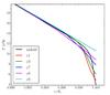 |
Fig. 2 Volume-averaged temperature in the outer 1% of the stellar radius for the non-accreting model (mdot0) and for the accreting models (cases e1 to e9) at time t = 3 × 10⁷ s. At this stage 1.9 × 1029 g has been accreted (3 × 10⁷ s of accretion at an accretion rate of 1 × 10⁻⁴M⊙ yr-1). Curves labelled e1−e9 correspond to the accreting calculations with varying eacc (see Table 1 for the specific internal energies of the accreted material). |
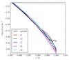 |
Fig. 3 Volume-averaged density in the outer 0.5% of the stellar radius for the models shown in Fig. 2. |
The increase in the temperature of the surface layers as eacc increases (see Fig. 2) affects the energy transport and the properties of the convection in the envelope. We first analyse the convective velocities for all considered models. These can be characterised by the averaged root-mean-square (rms) velocities vrms in the convective region. Figure 4 shows the rms velocities volume-weighted averaged in the θ-coordinate and time-averaged over 107 s. This time interval is sufficient for calculating time-averaged quantities because it equates to between ~17 and ~36 convective turnovers, depending on the models (see Table 1). The convective turnover time scale, τconv, can be defined by: 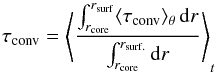 (3)where
 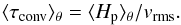 (4)Here, rcore and rsurf are the radius at the bottom and top of the convective zone, respectively, and Hp is the pressure scale height. The angle brackets with subscript θ denote volume-weighted averages in the θ-coordinate, and angle brackets with t subscript indicate a time-weighted average.
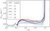 |
Fig. 4 Profile of the rms velocities volume-weighted averaged over θ and time-averaged over 107 s for the models shown in Fig. 2. |
Note in Fig. 4 that the large values of the rms velocities near the surface are due to the tangential component of the velocity of the flows that develop close to the outer boundary. In the following, we refer to cold, cases with entropy of the accreted material lower than the bulk entropy in the convective envelope (e1−e4), moderately hot if the accreted entropy is slightly higher (e5−e7) and hot cases if the accreted entropy is much higher (e8−e9). Cold cases to moderately hot accretion models tend to show a slight increase in convective velocities relative to the non-accreting model (black curve). Hot accretion cases (e8, e9) show a decrease in convective velocities in the bulk of the convective region. This decrease is also evident from the larger values of the convective turnover timescales given in Table 1. The radial profile of the rms of the radial velocity component shows the same trend as a function of the accreted entropy.
In addition to the convective velocities, an analysis of the enthalpy luminosity for the different simulations gives insight into the role of convection. The mean radial enthalpy luminosity in the convective zone is related to the energy transported by convection and is equivalent to the convective luminosity in the framework of the mixing-length theory. It is computed as 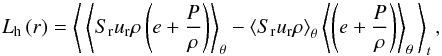 (5)where P is the pressure and Sr is the surface area of a cell at radius r (see Viallet et al. 2011). The second term on the r.h.s. of the equation accounts for non-zero mean vertical mass fluxes (Freytag et al. 1996), which can be important in the case of accretion. Figure 5 shows radial profiles of Lh, time-averaged over 2 × 10⁷ s, for the non-accreting (mdot0), cold (e1), and hot (e9) accreting cases. The behaviour of the enthalpy luminosity is similar to that found for the rms velocities. Both quantities show a significant decrease in the bulk of the convective zone for the hot accretion case (e9) compared to the non-accreting (mdot0) and cold accreting (e1) cases. Heating the surface layers of a convective star, as observed in Fig. 2 for the hot accretion cases, leads to a reduction of the rate of energy transport by convection compared to the cold and non-accreting cases. Surface cooling and steep temperature gradients near the surface drive convection in a stellar envelope. Adding heat to the surface locally changes (or even inverts) the temperature gradient, and therefore can inhibit convection. Despite the suppression of convection, calculation of the mean radiative luminosity Lrad as a function of radius2 shows that it remains by several orders of magnitudes smaller than Lh in the bulk of the convective zone for all simulations. This stems from the fact that the thermal profile and thus the radiative flux require a thermal relaxation timescale to adjust and eventually to compensate for the reduced efficiency of convection. An estimation of the thermal relaxation timescale of the upper layers (see Sect. 5) indicates that only layers with r/R> 0.99 have enough time to adjust during the total time of the simulations, i.e. 3 × 10⁷ s. Our interpretation and the consequences of the results are further analysed in the next sections.
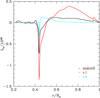 |
Fig. 5 Radial profiles of the time-averaged enthalpy luminosity (in erg s-1) in the non-accreting model (black line) and accreting cases e1 (red line) and e9 (cyan line). |
4. Distribution of accreted material
4.1. Numerical mass distribution
An additional interpretation of the results is provided by analysing how the accreted material is distributed throughout the stellar interior. We first approach the problem by comparing at a given time the mass in each radial shell to that in each corresponding shell in an otherwise identical non-accreting model. The result of this comparison is shown in Fig. 6 where the change in the mass of each shell ΔMacc, derived from the change in density, is expressed as a fraction of the total accreted mass Macc = ṀΔt. The quantity ΔMacc is calculated from the density and volume of the computational cells in a given radial shell (i.e. averaged over θ) and for a model at a given time (not time-averaged). Note that the sum of ΔMacc/Macc over all shells in the stellar model is equal to 1. The change in density of a cell comes from i) compression due to the addition of material in layers above, and ii) from the addition of the newly accreted material. Thus, the quantity ΔMacc/Macc is a measure of the net change in stellar density as a result of the accretion process and not just a measure of the mass added in each shell. Figure 6 shows the similarity of results with different accretion entropy in the range −30% ≤ δsacc ≤ 30% (cases e1 to e7). Higher accretion entropy, however, favours a density increase closer to the surface of the star. This trend is clearest in the hottest case, e9. We stress that the curves plotted in Fig. 6 and linking quantities that are defined in each shell are shown for the sake of illustrating the differences in the mass distribution between different accretion energy cases. While the details will depend on the resolution, the overall trends will not.
To better understand the difference between density variation due to compression of material and that due to mass addition, we use another method, namely tracer particles. The non-interacting particles trace out the path an infinitesimally small fluid element would follow with a given initial position subject to the velocity field calculated by MUSIC. We use a simple predictor-corrector method to integrate the particle positions. In order to determine each tracer particle’s motion between two timesteps, say n and n + 1, we first estimate the particle position at time n + 1/2 based only on the velocity field at time n. We then use this half-way position to find a more representative velocity for the whole time interval of the particle’s motion between the two timesteps.
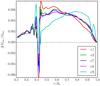 |
Fig. 6 Change in mass distribution in each radial shell of an accreting model relative to the non-accreting model for different values of eacc at time t = 3 × 10⁷ s. The reference model used to calculate ΔMacc is the non-accreting model at same age (see text, Sect. 4). |
To study the distribution of the accreted material we add the particles over time at the surface of the star at a fixed rate and over the accreting area Aacc. Examining the radial distribution of particles gives some insight into how the newly accreted material is distributed. Figure 7 shows the result of adding 75 000 tracer particles, at 200 s intervals and randomly distributed in the θ-direction within the accreting region, from the start of accretion until 1.5 × 10⁷ s. The grey scale applied to the particles indicates when they were added to the simulation, with darker particles being added earlier than lighter particles. The colour scale indicates the radial velocities. Motions characteristic of convection (see e.g. Stein & Nordlund 1998) can be seen with down flows, indicated by blue, and up flows, indicated by red. The left panel of the figure shows the distribution of particles in the low energy (e1) case, while the right panel shows the distribution of particles in the high energy (e9) case. In the low energy case the particles are distributed throughout the convective zone. In the high energy case they are concentrated in the outer 10% of the stellar radius. The few particles that penetrate deeper into the convective region in the latter case were added early in the accretion process and transported before the structure, subjected to the new accretion boundary condition, reached a steady state.
One can associate a mass to each particle to represent the amount of matter accreted, given the fixed rate at which these particles are added and the fixed mass accretion rate. We can thus derive a distribution of accreted mass from the particles. This mass distribution is shown in Fig. 8 and is compared to the accreted mass distribution based on the change in density. Note that the mass distribution for the e1 case plotted in Fig. 6 (red curve) slightly differs from the one plotted in Fig. 8 since they are not evaluated at the same time. The particle derived accreted mass distributions do not take into account the compression which occurs due to accretion. They should thus not necessarily match that derived from the density change.
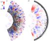 |
Fig. 7 Distribution of tracer particles accreted during 1.5 × 10⁷ s for the low energy (e1) and high energy accretion (e9) cases respectively. Colour scale is the radial velocity in units of cm s-1 and grey scale points show the position of the tracer particles. Velocities are instantaneous, i.e. not time-averaged. Blue indicates down flows, while red indicates up flows. Lighter coloured points correspond to more recently added tracer particles. Both snapshots are at a time t = 1.5 × 10⁷ s. |
In the e1 case the two methods based on density change and on particles respectively, show a similar distribution, however, the particles reveal that there is no mixing of accreted material in the radiative region. In the e9 case, the particle derived accretion mass distribution shows that the newly accreted material remains near the surface and does not mix into the deep convective region. This is consistent with having high entropy material above lower entropy material. The two mass distributions derived from the particles and from the density change are thus different, as shown in the bottom panel of Fig. 8.
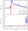 |
Fig. 8 Comparison of mass distributions between that derived from model density and that from particle distributions for the e1 (top panel) and e9 (bottom panel) models. The mass distributions are derived from the models displayed in Fig. 7 at time t = 1.5 × 10⁷ s. |
4.2. Comparison to the analytical model of Siess & Forestini (1996)
The only work we know that attempts to model the mass distribution resulting from accretion in stellar interiors is the work of Siess & Forestini (1996). These authors construct a complex analytical model to specify the accreted mass distribution in the framework of one dimensional stellar evolution models. It is interesting to compare predictions from their model to the results of our numerical experiments. Siess & Forestini (1996) define a radially dependent penetration function, f = ΔMacc/ ΔM∗, where ΔMacc and ΔM∗ are the accreted and initial mass in a given radial shell, respectively. The computation of f results from the integration of a differential equation (see Eq. (23) in Siess & Forestini 1996) that depends on quantities derived from the stellar model such as the pressure scale height, adiabatic gradient, and stellar radius and mass. In addition, the model contains several free parameters: ξ is the fraction of the Keplerian specific angular momentum of the accreted material, Ri− is the Richardson number, which must take negative values in convective regions, and ϵa is related to how quickly the accreted matter is thermalised (see Siess & Forestini 1996, for details about these parameters).
We can compute the equivalent of the penetration function f directly from our 2D simulations of accretion, because they provide the quantities ΔMacc and ΔM∗. This numerical penetration function can be compared to the semi-analytical values of f obtained from solving the differential equation of Siess & Forestini (1996). The quantity ΔMacc for the 2D simulations is derived from the density change and not from the particles since the latter, as already mentioned, only partially accounts for the effects of mass addition, omitting the effect of compression due to the addition of material. The former derivation thus provides a more realistic description of the net effect of mass accretion, which is what should count in a 1D stellar evolution calculation using a penetration function. The results are shown in Fig. 9 for the e1 and e9 accretion simulations. The dashed cyan (ξ = 0.015, Ri− = −1 × 10⁴, ϵa = 0.15) and maroon (ξ = 0.01, Ri− = −10, ϵa = 0.005) curves are our best attempts to fit the numerical results for the e1 and e9 cases respectively. The analytic penetration functions are poor fits to those derived from the 2D simulations. Despite many attempts, we find it difficult to match both the peak of the curve at the surface and the shape of the curve below the surface. Interestingly though, the best fit for the e9 case requires a smaller absolute value for Ri− than that needed for the e1 case. Small absolute values of this parameter correspond to a regime where convection is not very efficient, while large absolute values indicate efficient convection (Siess & Forestini 1996), in line with our findings in Sect. 3.
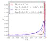 |
Fig. 9 Comparison between penetration functions derived from our 2D simulations and that from the analytic model of Siess & Forestini (1996). The figure shows a comparison for the e1 simulation (solid red curve) with our best fit analytic function (dashed cyan curve) and a comparison for the e9 simulation (solid blue curve) with our best fit analytic function (dashed maroon curve). |
Experimenting further, we note that we are able to better fit the shape of the penetration function for a lower accretion rate. We performed a 2D simulation with a mass accretion rate Ṁ = 10-6M⊙ yr-1 and low accreted entropy as in the e1 case. The corresponding analytical penetration function can fit the numerical results with a set of free parameters (ξ = 0.01, Ri− = −2.2 × 10³, ϵa = 0.15). The values of f very close to the surface remain, however, significantly higher than computed from the 2D simulation. We do not wish to push further such comparisons, which certainly remain limited as our numerical simulations do not account for deposition and inward transport of angular momentum. But the main lesson from such comparisons is that the Siess & Forestini (1996) formalism, in addition of being complicated for implementation in 1D stellar evolution code, requires fine tuning of the free parameters depending on the accretion details, and may break for extreme cases of high accretion and energy deposition rates.
5. Impact on one dimensional structure and evolution
The results from the 2D simulations presented in the previous sections can be used as guidance for the treatment of accretion in 1D stellar evolution calculations. They show that the redistribution of the accreted material within the convective envelope remains efficient for cold and even moderately hot accretion (e1 to e7 cases). These cases correspond to values of α (see Eq. (1)) ranging from ~0.01 (e1) to ~0.06 (e7). A different behaviour in terms of mass redistribution, rms velocities in the convective envelope and enthalpy flux is observed for the hottest cases investigated (e8 and e9), corresponding to values of α of ~0.1 for e8 and ~0.2 for e9. Note that, for a given initial stellar model, the exact value of eacc at which this change in behaviour is observed will likely depend on the accretion rate, the accreting surface area, the inflow velocity (see Sect. 2.2), as well as the boundary conditions and spatial resolution. Thus, the quantitative value of eacc (or α) at which this change in behaviour occurs is not very significant, only the qualitative effects highlighted by the 2D simulations is of importance. The visualisation, thanks to the tracer particles, of a hot layer produced at the surface of the accreting object due to the accumulation of high entropy material (see Fig. 7) raises several questions. First, what is the long-term effect of such a hot buffer zone on the structure and evolution of the accreting object? Second, since obviously the hot accreted material is prevented from sinking into the deeper layers, is the assumption of redistribution of accreted energy into the interior (Siess et al. 1997; Hartmann et al. 1997; Baraffe et al. 2012) able to mimic the effect of this hot layer at the surface?
We address these questions with our 1D Lyon stellar evolution code, assuming different treatments of accretion. The accreted mass is assumed to be redistributed over the entire structure, whether accretion is cold or hot (see Eq. (3) of Baraffe & Chabrier 2010)3. Starting from the 1D young Sun structure used for the initial model in the 2D simulations, we run 1D simulations with a constant accretion rate of Ṁ = 10-4M⊙ yr-1 for approximately 100 yr. This corresponds to the typical duration of high accretion bursts adopted in the framework of episodic accretion scenarios (Hosokawa et al. 2011; Baraffe et al. 2012). On one hand, we adopt a similar treatment to that described in Baraffe et al. (2009), Baraffe & Chabrier (2010) assuming cold accretion, equivalent to α = 0, and a hot accretion case assuming uniform redistribution within the stellar interior of the accretion energy, Ladd (see Eq. (1)), with α = 0.2 to correspond to the e9 case. The α = 0.2 case is relevant for the scenario developed by Baraffe et al. (2012) to explain some of the observed properties of FU Ori. Note that such a treatment assumes that the accreting star can freely radiate its energy over most of its photosphere (see also Hartmann et al. 1997). On the other hand, we adopt the treatment inspired by the results of the 2D simulation for the hottest case and impose the boundary condition that the surface luminosity Lsurf equals the accretion energy rate Ladd. This treatment is similar to the one adopted by Mercer-Smith et al. (1984). In this case, only the outer boundary condition is modified and no accretion energy is redistributed within the stellar interior. This forces the value of the effective temperature (the surface temperature Tsurf) to tend toward the value  . It is also equivalent to the boundary condition used at the top of the domain of the 2D simulations, where it is assumed that the surface radiates a flux F = σT4 with T the temperature of the cells at the top of the domain (see Sect. 2.1). Adopting α = 0.2 yields Ladd ~ 100 L⊙, a value comparable to the surface luminosity of the e9 case displayed in Table 1.
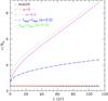 |
Fig. 10 Evolution of the radius of non-accreting and accreting young Sun models calculated with the 1D stellar evolution code. The non-accreting model is shown as the black line. Coloured curves indicate accreting models with a rate Ṁ = 10-4M⊙ yr-1 assuming different treatments of accretion: cold accretion (red dash); hot accretion assuming uniform redistribution within the stellar interior of the accretion energy rate Ladd with α = 0.2 (magenta dash-dot ); hot accretion assuming an accretion boundary condition Lsurf = Ladd with α = 0.2 (blue dash) and α = 0.3 (green dot). |
The results displayed in Fig. 10 show the evolution of the radius in the 1D models with two different treatments of hot accretion: uniform energy redistribution and outer accretion boundary condition. In both cases the two different treatments of hot accretion yield a rapid expansion of the accreting object, with the expansion first proceeding in the outer surface layers close to the photosphere, given their much shorter relaxation timescale compared to the deeper layers. Figure 10 shows that for the same rate of energy added to the object through accretion, Ladd, a model assuming uniform redistribution of the energy within the interior (dash-dot magenta curve) overestimates the growth in the radius compared to a model assuming a more realistic accretion boundary condition where hot accreted material cannot sink and produces a hot surface layer (long dash blue curve). In order to obtain a similar evolution with an accretion boundary condition as obtained with the assumption of energy redistribution within the interior, one needs to increase by a factor 1.5 the amount of accretion energy transferred to the star, corresponding to a value of α = 0.3 (green dotted curve in Fig. 10).
Imposing an accretion boundary yields rapid heating of the photosphere and of the layers below. This heating results in the expansion of the outer layers, which starts after ~1 yr of evolution. The heating and thus the modification of the thermal profile propagates from the surface to deeper layers on a thermal relaxation timescale τth, which can be estimated by 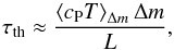 (6)where Δm is the mass of the layers considered below the surface, cP the specific heat at constant pressure and the brackets ⟨ ⟩ Δm denote the average over these layers. With the boundary condition that L = Ladd with α = 0.2, modification of the thermal profile in the corresponding 1D simulation is observed for the very top layers with a fractional mass mr/M ≳ 0.9998 after about 1 yr of evolution. This is consistent with the estimate of the thermal timescale of these layers τth ~ 1 yr derived from Eq. (6) and with the change in the thermal profile illustrated in Fig. 2 for the 2D simulations. After around 100 yr of evolution, the 1D model with the accreting boundary condition shows a modification of its thermal profile for layers down to a depth mr/M ~ 0.985, consistent with their thermal timescale τth ~ 150 yr. The expansion of models with a hot accretion condition displayed in Fig. 10 stems from the expansion of these upper layers characterised by a fast adjustment timescale. Note that the thermal timescale of the whole star, given by the Kelvin-Helmotz timescale τKH = GM2/ (RL), is around 4 Myr for the initial young Sun (non-accreting) model and about 0.1 Myr for the accreting model with the accretion boundary condition and α = 0.2 (it is shorter in the latter case because of the higher imposed surface luminosity).
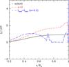 |
Fig. 11 Radial profile of the luminosity (in erg s-1) in the young Sun model after 1 yr of evolution, based on 1D stellar evolution calculations. The black solid line represented the non-accreting model. Coloured curves indicate accreting models with a rate Ṁ = 10-4M⊙ yr-1 assuming cold accretion (red dash-dot) and hot accretion with an accretion boundary condition Lsurf = Ladd with α = 0.2 (blue dash). |
To further compare with the 2D results, we analyse the total luminosity profile as a function of radius for 1D models in Fig. 11 after 1 yr of simulation starting from the same initial model. This is similar to the total time spanned by the 2D simulations with accretion (3 × 10⁷ s). The non-accreting model (black curve) shows a profile characteristic of a pre-Main Sequence star contracting as a whole and with no nuclear energy source, with the luminosity L powered by local gravitational energy due to contraction  and by change in internal energy
  :
:  (7)The total luminosity in the convective envelope is representative of the convective luminosity, because energy transport is dominated by convection and the contribution from radiation is negligible in the non-accreting model. The cold accretion case shows a similar behaviour, but in addition to the contraction of the whole object, there is also a contribution to the gravitational energy due to the mixing of cold entropy material in the interior, as visualised in the 2D model for the e1 case in Fig. 7. As shown in Fig. 11, this yields a higher interior luminosity compared to the non-accreting case. An equivalent result is found in the 2D cold and moderately hot accretion cases. This behaviour observed in the 1D models explains the higher enthalpy luminosity in the 2D e1 model relative to the 2D non-accreting model (compare the e1 case to the non-accreting case in Fig. 5). For the hot accretion case based on the accretion boundary condition (blue dashed curve in Fig. 11), the luminosity significantly decreases within the bulk of the convective zone, as observed for the 2D e9 case in Fig. 5. Inspection of the different terms contributing to the luminosity in the 1D model indicates a slight expansion of the outer envelope, i.e.
  , contributing negatively to the luminosity and counterbalancing the positive contribution from the deeper contracting regions. Such contributions can already be seen after 1 yr of evolution, even if the change in total radius remains small. As the 1D model with the accretion boundary condition further evolves and expands, examination of its interior structure shows that the top boundary of the convective zone recedes from the surface, as also noted by Prialnik & Livio (1985). Additionally, in the convective zone, the energy transport by convection becomes less efficient and the contribution of radiative transport increases.
The parallel between the 1D and 2D results is interesting. First, it indicates that the 1D treatment of cold accretion assumed in previous studies is roughly consistent with the 2D results, with efficient redistribution of the accreted mass within the interior and similar effect of accretion on the luminosity in the convective envelope. Second, for hot accretion, the assumption of redistribution of the accreted energy within the interior seems to overestimate the effect on the structure, namely the expansion of the accreting object, for a given total amount of accretion energy gained. An accretion boundary condition assuming Lsurf = Ladd seems more realistic and more in line with the 2D results. However, despite the quite unphysical picture represented by the assumption of accreted energy redistribution within the interior in the case of hot accretion, it can mimic the effect described by the 2D simulations, assuming a smaller amount of the accretion energy is transported deep into the interior.
6. Discussion and conclusion
Our main results can be summarised as follows. The usual assumption made in 1D stellar evolution codes of instantaneous and homogeneous redistribution of accreted material within the interior of the accreting object is supported by the multi-D simulations in the case of low to moderately high entropy accreted material. In this context, low or high entropy refers to the value of the entropy of the accreted material compared to the entropy of the adiabatic convective envelope. For high entropy material, the assumption of energy redistribution within the interior is physically wrong and opposite to results depicted by the multi-D simulations, namely there is an accumulation of hot material at the surface that does not sink and instead produces a hot surface layer. The presence of this hot surface layer tends to suppress convection in the envelope. An accretion boundary condition such as Lsurf = Ladd, in the case of hot accretion, provides a more physical treatment. For a given amount of accreted energy transferred to the accreting object, a treatment assuming accretion energy redistribution throughout the stellar interior significantly overestimates the effects on the stellar structure, and in particular on the resulting expansion.
Given the lack of knowledge regarding the amount of accretion energy transferred to the accreting object, a systematic analysis is required to explore the impact of these results. Work is in progress to understand how the use of the accretion boundary condition inspired by this work will affect the conclusions of previous studies based on the former treatment for hot accretion (Baraffe et al. 2009, 2012; Hosokawa et al. 2011) and the interpretation of observations relying on hot accretion scenario (e.g. Hartmann et al. 2011).
The outcome of this work depends on various assumptions and uncertainties that we discuss below. The first question regards the impact of using 2D instead of 3D geometry. It is well known that 2D description of turbulent convection in stars gives different results compared to 3D simulations (see e.g. Meakin & Arnett 2007, and references therein). Exploring the same range of parameters used in the present study with 3D simulations is currently unaffordable. We do not, however, expect the qualitative results to be altered by the limitations inherent to the 2D description of convection.
One of the most interesting results is the dependence of behaviour on the entropy of the accreted material and the subsequent formation of a hot surface layer. We find no obvious argument why such layer would not form in 3D, though it could conceivably change the value of α at which this happens. Moving to 3D geometry will have an impact on the development of meridional flows at the surface of the accreting objects and how accreted material is redistributed over its surface. But given our assumption that the accreting area covers the entire surface of the star, inspired by the boundary layer simulations of Kley & Lin (1996) or by the idea of a spreading layer surrounding the whole accreting object, the transition from 2D to 3D geometry should not change the general picture described in this paper.
Extending the simulations to 3D could be relevant if the accreting surface area does not cover the whole star, but only a fraction of it. This is an assumption that should be considered in future work, as it will change the outer boundary conditions and how the accreting star radiates its energy. Extending the simulations to 3D would also be important if including the accretion of angular momentum and analysing its redistribution within the stellar interior. This problem has not been addressed, because our 2D simulations do not account for rotation of the object and angular momentum of the accreting material. Given our extremely poor knowledge regarding the rotational properties of embedded protostars and of the loss of angular momentum of material in a boundary layer, such a simple configuration may be realistic in some cases, and at the very least a good baseline for comparison with potentially more sophisticated future models.
The treatment of the surface layers and of the boundary conditions, as well as the grid resolution, are other sources of uncertainty. In a parallel study, we are investigating the sensitivity of convection properties to the grid resolution and the boundary conditions in the same stellar model as used in this work (Pratt et al. 2016). We do expect quantitative results such as the value of eacc that characterises the change in behaviour in the simulations and the formation of a hot surface layer, the surface temperature and the thickness of the high entropy surface layer of accreted material in the case of hot accretion to depend on the setup (i.e. treatment of surface layers, boundary conditions and/or grid resolution). But these setup effects may be covered by the large uncertainty contained in the free parameter α regarding the amount of accretion energy transferred onto the surface of the accreting object.
One key assumption of our study though concerns the treatment of accretion through a simple accretion boundary. Further exploration of different types of boundaries to account for the accretion process are required to determine the impact of our assumption. Finally, present simulations are limited by the use of a fixed spatial grid that does not allow the stellar radius to vary. The 1D simulation including an accretion boundary condition indicates that after about 1 yr, the envelope starts to expand and the radius increases. For this reason, it is incorrect to simulate longer times with our multi-D simulations, unless some grid movement is allowed for, because our multi-D framework does not account for the expansion of the star in the hot accretion case. We are exploring the possibility of implementing a moving grid in MUSIC, which would be required not only for accretion studies but also for investigating stellar pulsation problems.
This work is the first attempt to describe the multi-dimensional structure of accreting young stars. Understanding the accretion process from first principles with numerical simulations is a formidable physical and numerical challenge that we do not pretend to fully address with the present multi-dimensional simulations. Our motivation is to use multi-dimensional simulations to analyse the validity of accretion treatments used in 1D stellar evolution studies and to improve such treatments for further studies and for the interpretation of observations. More broadly, our motivation is to perform similar multi-dimensional studies for other key processes of stellar evolution such as convective overshooting, rotation, or pulsation. This pioneering work hopefully shows the potential of using time implicit multi-D simulations to improve our understanding of stellar evolution.
Conserved variables are however used to solve the conservation equations (see Viallet et al. 2016, for details).
See Viallet et al. (2011) for the calculation of the mean radiative luminosity.
Note that the Lyon stellar evolution code is based on the Lagrangian coordinate mr, i.e. the mass enclosed in a sphere of radius r, and needs to account for the change in entropy due to mass variation during the accretion process as done in e.g. Hayashi et al. (1965), Baraffe & Chabrier (2010).
Acknowledgments
I.B. would like to dedicate this work to Francesco Palla who recently passed away. Part of this work was funded by the Royal Society Wolfson Merit award WM090065, the French Programme National de Physique Stellaire (PNPS) and Programme National Hautes Énergies (PNHE), and by the European Research Council through grants ERC-AdG No. 320478-TOFU and ERC-AdG No. 341157-COCO2CASA. This work used the DiRAC Complexity system, operated by the University of Leicester IT Services, which forms part of the STFC DiRAC HPC Facility (www.dirac.ac.uk). This equipment is funded by BIS National E-Infrastructure capital grant ST/K000373/1 and STFC DiRAC Operations grant ST/K0003259/1. DiRAC is part of the National E-Infrastructure. This work also used the University of Exeter Supercomputer, a DiRAC Facility jointly funded by STFC, the Large Facilities Capital Fund of BIS and the University of Exeter.
References
- Balsara, D. S., Fisker, J. L., Godon, P., & Sion, E. M. 2009, ApJ, 702, 1536 [NASA ADS] [CrossRef] [Google Scholar]
- Baraffe, I., & Chabrier, G. 2010, A&A, 521, A44 [NASA ADS] [CrossRef] [EDP Sciences] [Google Scholar]
- Baraffe, I., & El Eid, M. F. 1991, A&A, 245, 548 [NASA ADS] [Google Scholar]
- Baraffe, I., Chabrier, G., Allard, F., & Hauschildt, P. H. 1998, A&A, 337, 403 [NASA ADS] [Google Scholar]
- Baraffe, I., Chabrier, G., & Gallardo, J. 2009, ApJ, 702, L27 [NASA ADS] [CrossRef] [Google Scholar]
- Baraffe, I., Vorobyov, E., & Chabrier, G. 2012, ApJ, 756, 118 [NASA ADS] [CrossRef] [Google Scholar]
- Chabrier, G., & Baraffe, I. 1997, A&A, 327, 1039 [NASA ADS] [Google Scholar]
- Freytag, B., Ludwig, H.-G., & Steffen, M. 1996, A&A, 313, 497 [Google Scholar]
- Hartmann, L., Cassen, P., & Kenyon, S. J. 1997, ApJ, 475, 770 [NASA ADS] [CrossRef] [Google Scholar]
- Hartmann, L., Zhu, Z., & Calvet, N. 2011, ArXiv e-prints [arXiv:1106.3343] [Google Scholar]
- Hayashi, C., Hōshi, R., & Sugimoto, D. 1965, Prog. Theor. Phys., 34, 885 [NASA ADS] [CrossRef] [Google Scholar]
- Hertfelder, M., Kley, W., Suleimanov, V., & Werner, K. 2013, A&A, 560, A56 [NASA ADS] [CrossRef] [EDP Sciences] [Google Scholar]
- Hosokawa, T., Yorke, H. W., & Omukai, K. 2010, ApJ, 721, 478 [NASA ADS] [CrossRef] [Google Scholar]
- Hosokawa, T., Offner, S. S. R., & Krumholz, M. R. 2011, ApJ, 738, 140 [NASA ADS] [CrossRef] [Google Scholar]
- Inogamov, N. A., & Sunyaev, R. A. 1999, Astron. Lett., 25, 269 [NASA ADS] [Google Scholar]
- Kippenhahn, R., & Thomas, H.-C. 1978, A&A, 63, 265 [NASA ADS] [Google Scholar]
- Kley, W., & Hensler, G. 1987, A&A, 172, 124 [NASA ADS] [Google Scholar]
- Kley, W., & Lin, D. N. C. 1996, ApJ, 461, 933 [NASA ADS] [CrossRef] [Google Scholar]
- Kutter, G. S., & Sparks, W. M. 1987, ApJ, 321, 386 [NASA ADS] [CrossRef] [Google Scholar]
- Meakin, C. A., & Arnett, D. 2007, ApJ, 667, 448 [NASA ADS] [CrossRef] [Google Scholar]
- Mercer-Smith, J. A., Cameron, A. G. W., & Epstein, R. I. 1984, ApJ, 279, 363 [NASA ADS] [CrossRef] [Google Scholar]
- Palla, F., & Stahler, S. W. 1992, ApJ, 392, 667 [NASA ADS] [CrossRef] [Google Scholar]
- Piro, A. L., & Bildsten, L. 2004, ApJ, 610, 977 [NASA ADS] [CrossRef] [Google Scholar]
- Pratt, J., Baraffe, I., Goffrey, T., et al. 2016, A&A, submitted [Google Scholar]
- Prialnik, D., & Livio, M. 1985, MNRAS, 216, 37 [NASA ADS] [Google Scholar]
- Pringle, J. E. 1981, ARA&A, 19, 137 [NASA ADS] [CrossRef] [Google Scholar]
- Shaviv, G., & Starrfield, S. 1988, ApJ, 335, 383 [NASA ADS] [CrossRef] [Google Scholar]
- Siess, L., & Forestini, M. 1996, A&A, 308, 472 [NASA ADS] [Google Scholar]
- Siess, L., Forestini, M., & Bertout, C. 1997, A&A, 326, 1001 [NASA ADS] [Google Scholar]
- Stein, R. F., & Nordlund, Å. 1998, ApJ, 499, 914 [Google Scholar]
- Viallet, M., Baraffe, I., & Walder, R. 2011, A&A, 531, A86 [NASA ADS] [CrossRef] [EDP Sciences] [Google Scholar]
- Viallet, M., Baraffe, I., & Walder, R. 2013, A&A, 555, A81 [NASA ADS] [CrossRef] [EDP Sciences] [Google Scholar]
- Viallet, M., Goffrey, T., Baraffe, I., et al. 2016, A&A, 586, A153 [NASA ADS] [CrossRef] [EDP Sciences] [Google Scholar]
All Tables
All Figures
|
Fig. 1 Visualisation of the computational mesh. On the right is a zoom of the near surface mesh showing the geometrically decreasing radial spacing. Note that the changes in grid-lines are a result of the rasterisation process to generate the figure and not indicative of a change in actual grid geometry. |
| In the text | |
|
Fig. 2 Volume-averaged temperature in the outer 1% of the stellar radius for the non-accreting model (mdot0) and for the accreting models (cases e1 to e9) at time t = 3 × 10⁷ s. At this stage 1.9 × 1029 g has been accreted (3 × 10⁷ s of accretion at an accretion rate of 1 × 10⁻⁴M⊙ yr-1). Curves labelled e1−e9 correspond to the accreting calculations with varying eacc (see Table 1 for the specific internal energies of the accreted material). |
| In the text | |
|
Fig. 3 Volume-averaged density in the outer 0.5% of the stellar radius for the models shown in Fig. 2. |
| In the text | |
|
Fig. 4 Profile of the rms velocities volume-weighted averaged over θ and time-averaged over 107 s for the models shown in Fig. 2. |
| In the text | |
|
Fig. 5 Radial profiles of the time-averaged enthalpy luminosity (in erg s-1) in the non-accreting model (black line) and accreting cases e1 (red line) and e9 (cyan line). |
| In the text | |
|
Fig. 6 Change in mass distribution in each radial shell of an accreting model relative to the non-accreting model for different values of eacc at time t = 3 × 10⁷ s. The reference model used to calculate ΔMacc is the non-accreting model at same age (see text, Sect. 4). |
| In the text | |
|
Fig. 7 Distribution of tracer particles accreted during 1.5 × 10⁷ s for the low energy (e1) and high energy accretion (e9) cases respectively. Colour scale is the radial velocity in units of cm s-1 and grey scale points show the position of the tracer particles. Velocities are instantaneous, i.e. not time-averaged. Blue indicates down flows, while red indicates up flows. Lighter coloured points correspond to more recently added tracer particles. Both snapshots are at a time t = 1.5 × 10⁷ s. |
| In the text | |
|
Fig. 8 Comparison of mass distributions between that derived from model density and that from particle distributions for the e1 (top panel) and e9 (bottom panel) models. The mass distributions are derived from the models displayed in Fig. 7 at time t = 1.5 × 10⁷ s. |
| In the text | |
|
Fig. 9 Comparison between penetration functions derived from our 2D simulations and that from the analytic model of Siess & Forestini (1996). The figure shows a comparison for the e1 simulation (solid red curve) with our best fit analytic function (dashed cyan curve) and a comparison for the e9 simulation (solid blue curve) with our best fit analytic function (dashed maroon curve). |
| In the text | |
|
Fig. 10 Evolution of the radius of non-accreting and accreting young Sun models calculated with the 1D stellar evolution code. The non-accreting model is shown as the black line. Coloured curves indicate accreting models with a rate Ṁ = 10-4M⊙ yr-1 assuming different treatments of accretion: cold accretion (red dash); hot accretion assuming uniform redistribution within the stellar interior of the accretion energy rate Ladd with α = 0.2 (magenta dash-dot ); hot accretion assuming an accretion boundary condition Lsurf = Ladd with α = 0.2 (blue dash) and α = 0.3 (green dot). |
| In the text | |
|
Fig. 11 Radial profile of the luminosity (in erg s-1) in the young Sun model after 1 yr of evolution, based on 1D stellar evolution calculations. The black solid line represented the non-accreting model. Coloured curves indicate accreting models with a rate Ṁ = 10-4M⊙ yr-1 assuming cold accretion (red dash-dot) and hot accretion with an accretion boundary condition Lsurf = Ladd with α = 0.2 (blue dash). |
| In the text | |
Current usage metrics show cumulative count of Article Views (full-text article views including HTML views, PDF and ePub downloads, according to the available data) and Abstracts Views on Vision4Press platform.
Data correspond to usage on the plateform after 2015. The current usage metrics is available 48-96 hours after online publication and is updated daily on week days.
Initial download of the metrics may take a while.