| Issue |
A&A
Volume 588, April 2016
|
|
|---|---|---|
| Article Number | A56 | |
| Number of page(s) | 18 | |
| Section | Stellar atmospheres | |
| DOI | https://doi.org/10.1051/0004-6361/201528026 | |
| Published online | 17 March 2016 | |
Short-term variability and mass loss in Be stars
I. BRITE satellite photometry of η and μ Centauri⋆
1
European Organisation for Astronomical Research in the Southern Hemisphere
(ESO), Karl-Schwarzschild-Str. 2,
85748
Garching,
Germany
e-mail:
This email address is being protected from spambots. You need JavaScript enabled to view it.
2
European Organisation for Astronomical Research in the Southern
Hemisphere (ESO), Casilla 19001, Santiago 19, Chile
3
Astronomical Institute, Wrocław University,
Kopernika 11, 51-622
Wrocław,
Poland
4
Instituto de Astronomia, Geofísica e Ciências Atmosféricas,
Universidade de São Paulo, Rua do Matão 1226, Cidade Universitária,
05508-900
São Paulo, SP, Brazil
5
Département de physique and Centre de Recherche en Astrophysique
du Québec (CRAQ), Université de Montréal, CP 6128, Succ. Centre-Ville, Montréal, Québec, H3C
3J7, Canada
6
Department of Physics, Royal Military College of Canada, PO Box 17000,
Stn Forces, Kingston, Ontario
K7K 7B4,
Canada
7
Institute of Astronomy, University of Vienna, Universitätsring
1, 1010
Vienna,
Austria
8
Nicolaus Copernicus Astronomical Center, ul. Bartycka
18, 00-716
Warsaw,
Poland
9 Department of Physics and Astronomy, University of British
Columbia, Vancouver, BC V6T1Z1, Canada
10
Institute of Automatic Control, Silesian University of
Technology, Gliwice,
Poland
11
Department of Astronomy & Astrophysics, University of
Toronto, 50 St. George
St, Toronto,
Ontario, M5S 3H4, Canada
Received: 21 December 2015
Accepted: 1 February 2016
Abstract
Context. Empirical evidence for the involvement of nonradial pulsations (NRPs) in the mass loss from Be stars ranges from (i) a singular case (μ Cen) of repetitive mass ejections triggered by multi-mode beating to (ii) several photometric reports about enormous numbers of pulsation modes that suddenly appear during outbursts and on to (iii) effective single-mode pulsators.
Aims. The purpose of this study is to develop a more detailed empirical description of the star-to-disk mass transfer and to check the hypothesis that spates of transient nonradial pulsation modes accompany and even drive mass-loss episodes.
Methods. The BRITE Constellation of nanosatellites was used to obtain mmag photometry of the Be stars η and μ Cen.
Results. In the low-inclination star μ Cen, light pollution by variable amounts of near-stellar matter prevented any new insights into the variability and other properties of the central star. In the equator-on star η Cen, BRITE photometry and Heros echelle spectroscopy from the 1990s reveal an intricate clockwork of star-disk interactions. The mass transfer is modulated with the frequency difference of two NRP modes and an amplitude three times as large as the amplitude sum of the two NRP modes. This process feeds a high-amplitude circumstellar activity running with the incoherent and slightly lower so-called Štefl frequency. The mass-loss-modulation cycles are tightly coupled to variations in the value of the Štefl frequency and in its amplitude, albeit with strongly drifting phase differences.
Conclusions. The observations are well described by the decomposition of the mass loss into a pulsation-related engine in the star and a viscosity-dominated engine in the circumstellar disk. Arguments are developed that large-scale gas-circulation flows occur at the interface. The propagation rates of these eddies manifest themselves as Štefl frequencies. Bursts in power spectra during mass-loss events can be understood as the noise inherent to these gas flows.
Key words: circumstellar matter / stars: emission-line, Be / stars: mass-loss / stars: oscillations / stars: individual:ηCentauri / stars: individual:μCentauri
Based on data collected by the BRITE-Constellation satellite mission, built, launched and operated thanks to support from the Austrian Aeronautics and Space Agency and the University of Vienna, the Canadian Space Agency (CSA), and the Foundation for Polish Science & Technology (FNiTP MNiSW) and National Science Centre (NCN). Based in part also on observations collected at the European Organisation for Astronomical Research in the Southern Hemisphere under ESO programme 093.D-0367(A).
© ESO, 2016
1. Introduction
Be stars are one of the most ornate showcases of stellar physics along the entire main sequence: they display extreme rotation, nonradial g- and p-mode pulsation, outbursts, and high-speed winds. This is completed by the emission line-forming circumstellar disks that Be stars build as the screens onto which they can project their activities. These decretion disks are not just the opposite of accretion disks. Instead of powering high-energy jets to dispose of excess angular momentum, they viscously reshuffle specific angular momentum such that at least a fraction of the available matter can reach Keplerian orbits. Once elevated, they slowly drift away, sometimes in complex large-scale undulations. Be stars avoid close companions (unless they have swallowed them at an early moment) and do not sustain large-scale magnetic fields. The full Be-star story is told by Rivinius et al. (2013b) – as best as it can be done today.
Most notably, the physical process that enables Be stars to form circumstellar Keplerian disks is not finally identified. This challenge decomposes into two parts. The first one is to determine the engine that accelerates stellar matter such that it either orbits the star or drifts away from it. A second engine is needed to increase the specific angular momentum of this now circumstellar matter so that it can reach Keplerian orbits with larger radii, thereby forming a fully developed, slowly expanding Keplerian disk.
Even at typically ≥70% of the critical velocity (Fig. 9 in Rivinius et al. 2013b), rotation alone is not sufficient but most probably a necessary part of this second engine. Radiative winds do not play a major role because they are very weak in B-type main-sequence stars (Prinja 1989; Krtička 2014). In Be stars, UV wind lines are actually stronger than in B stars without circumstellar disks (Grady et al. 1989; Prinja 1989). But the aspect dependence (Grady et al. 1987) suggests that Be winds are stronger because they are more easily launched in the zero-gravity environment of the disk (see also Rivinius et al. 2013b).
Since the first discoveries (Baade 1982; Bolton 1982) of nonradial pulsations (NRPs) in Be stars, it has been hoped that they might provide the missing angular momentum and energy to lift stellar matter into circumstellar orbits. The variability of the emission-line strength, which may drop to zero, suggesting the complete dispersal of the disk (e.g., Wisniewski et al. 2010; Carciofi et al. 2012), and observations of discrete mass loss events in light curves (Huat et al. 2009), spectra (Peters 1986; Baade et al. 1988), and polarization (Hayes & Guinan 1984; Guinan & Hayes 1984) have led to the notion that much, if not all, of the star-to-disk mass-transfer process is episodic.
Indications were found early in the studies that outbursts and changes in the pulsation behavior of Be stars may be correlated (Bolton 1982; Penrod 1986). But in spite of considerable and diverse efforts over more than 30 yr, only one case has become known, in which NRPs are directly responsible for mass-loss episodes. Rivinius et al. (1998a) found that during phases of constructive superposition of the velocity field of the strongest mode of μ Cen with that of the second- or third-strongest mode the Hα line emission is enhanced, whereas the co-addition of the two weaker modes does not have this effect. Since the sum of the amplitudes a2 and a3 is smaller than a1 + a2 and a1 + a3 while all three modes have the same indices ℓ and m, the evidence seemed compelling that in μ Cen the beating of NRP modes, with frequencies close to 2 c/d, causes mass-loss events.
After matter has left the star, the viscous decretion disk (VDD) model (Lee et al. 1991) is generally acknowledged to give the best current description of the build-up process of the disk and its evolution (Carciofi et al. 2012; Haubois et al. 2012, 2014). It seems to be the solution to the second part of the quest for understanding of the Be phenomenon, namely how Be stars develop Keplerian disks.
Other observational studies have reported somewhat different relations but have drawn essentially the same conclusion, namely that (some) Be stars owe their disks to (the combination of rapid rotation and) nonradial pulsation. These examples are discussed below after some additional empirical arguments have been developed, so that they enable a different interpretation, inspired by the variability of η and μ Cen and as first anticipated by Rivinius (2013).
The complexity of the matter is highlighted by the fully negative results to date of searches for μ Cen analogs. Moreover, 28 ω CMa is perhaps the spectroscopically best-established single-mode pulsator among Be stars (Štefl et al. 2003b). And yet it shows a highly variable Hα emission-line strength and, therefore, mass-loss rate. However, at 7–9 yr (Štefl et al. 2003a; Carciofi et al. 2012), the repetition time of its outbursts is much more than an order of magnitude longer than in μ Cen.
On the other hand, μ Cen is one of the closest Be stars, and it would be odd if it were a singular case. Perhaps, the MACHO database (Keller et al. 2003) is a rich source of μ Cen analogs. Many of the false-alarm lensing events therein were due to outbursts of Be stars that satisfied the lensing selection criteria: roughly color-neutral brightening with an approximately symmetric light curve. In some cases, the outbursts repeated semi-regularly, which might be the signature of multi-mode beating. The OGLE database could harbor a similar bonanza (Mennickent et al. 2002), and the same may hold for the ASAS database (Pojmanski et al. 2005).
In short, Be stars require one engine to expel matter and a second to arrange the ejecta in a slowly outflowing Keplerian disk. Detailed comparisons of model calculations and observations have established the VDD model as the basis from which to further explore the disk properties. The broad acceptance of the NRP hypothesis for the inner engine rests on much circumstantial evidence, but also on the lack of other ideas. The interface between these two engines is largely unexplained territory.
One of the assumptions, on which the BRITE project is built, is that extensive series of high-quality spectra can be obtained for bright stars or are already available. The present study takes advantage of the existing spectra of η and μ Cen. Both have been intensively monitored with the Heros spectrograph (Kaufer et al. 1997; Schmutz et al. 1997) in the 1990s. This is the first paper in a series of studies revisiting the variability of Be stars with space photometers. The next study (Rivinius et al., in prep., hereafter “Paper II”) re-analyses Kepler observations. The results complement, and partly extend, those developed in this work.
Before presenting the BRITE observations (Sect. 3), the method used for their time-series analysis (Sect. 4), the results (Sect. 5), their analysis (Sect. 6) and discussion (Sect. 7), and finally the conclusions (Sect. 8), it is useful to describe in the next section a process that has so far not required and has therefore not received much attention. But to understanding the observations presented in this paper, it is of central importance.
2. Štefl frequencies
2.1. Spectroscopic signatures
Nearly 20 yr ago, Štefl et al. (1998) discovered that, during outbursts (periods of temporarily enhanced Hα line emission), the Be stars 28 ω CMa (see also Štefl et al. 2000,B2 IV-Ve) and μ Cen (B2 Ve) develop variability in the profiles of spectral lines that normally form above the photosphere (e.g., Mg II 448.1, Si II 634.7, etc. in absorption, the violet-to-red emission-peak ratio, V/R, of Fe II 531.6, and the mode of Balmer emission-line profiles). In agreement with this, the variability was confined to projected velocities above the equatorial level. (This agreement does not necessarily imply confirmation because the structures involved may have their own associated velocity field (as in pulsations)). The super-photospheric location was also observationally supported by Rivinius et al. (1998b), who found that the violet-to-red ratio of double-peaked emission lines (V/R) in μ Cen is also part of this variability.
In both stars, these temporary so-called Štefl frequencies are about 10–20% lower than a nearby strong stellar frequency, which the underlying line-profile variability unambiguously identified to be due to nonradial pulsation.
Štefl et al. (1998) suspected η Cen to be a third case. This was confirmed by Rivinius et al. (2003), as described in more detail in Sect. 6.4.2. An interesting difference with respect to the other two stars is that in η Cen the Štefl frequency seems to be permanent and of much larger amplitude than the stellar pulsations. Rivinius et al. (2003) also added κ CMa as a fourth Be star with transient frequencies. Using several lines, they not only illustrated (their Fig. 15) in more detail that the velocity range of the features substantially exceeds ± vsini, but also that quasi-periodic line profile-crossing features are associated with this variability.
The two discovery publications received hardly any citations, and even the authors themselves only proposed (Rivinius et al. 1998b) the very qualitative idea of an ejected cloud with an orbit that has not yet been circularized before merging with the disk. It is not clear how this notion can account for the permanent presence of a Štefl frequency in η Cen (see also the next subsection for the somewhat similar case of Achernar). Therefore, Štefl frequencies mark one of the largest gaps in the observational knowledge of Be stars. They appear to arise from the interface between star and disk, the engine generating them is probably fed by the mass-loss process, and the latter may involve stellar NRP modes of slightly higher frequency. Compared to stellar oscillations, Štefl frequencies may carry relatively little general information about the central star.
2.2. Photometric signatures
Before BRITE, no long series of high-quality photometric observations were available for any of the stars with spectroscopic Štefl frequencies. Without spectroscopic diagnostic support, these frequencies can be slightly treacherous because they may be mistaken for stellar pulsations. However, this additional difficulty does not prevent the identification of Štefl frequencies in photometric data.
The best test case at hand are the observations of α Eri (Achernar; B4) with the Solar Mass Ejection Imager (SMEI). Goss et al. (2011) have published a very elaborate analysis, which concludes that there are only two significant frequencies. F1 = 0.775 c/d is fairly constant over nearly five years while F2 = 0.725 c/d exhibits significant shifts in frequency and phase, which moreover are associated with apparent overall brightness variations. Both variabilities have time-dependent amplitudes. With a factor of 8, the amplitude variation of F2 is the strongest, so that F2 even dropped below detectability.
The nature of the SMEI observations does not readily permit detection of long-term brightness variations with confidence. Moreover, α Eri is observed at a large inclination angle but not equator-on. Model calulations by Haubois et al. (2012; their Fig. 13) suggest that in this case the response in optical light to the ejection of matter is very weak. Therefore, the annual SMEI light curves are not sufficient to infer the occurrence of an outburst at the onset in 2004 of the various anomalies described above. But Rivinius et al. (2013a) reported a strengthening of the Hα equivalent width at the end of 2004, which is the signature of an increased amount of matter close to the central star.
Characteristic frequencies (in c/d) of Be stars known to exhibit Štefl frequencies.
Figure 2 of Goss et al. (2011) is of special interest: Although it covers 30 d, it exhibits no indication of the nominal beat period of about 20 d for F1 and F2. This implies quite immediately that one or both of the two variations are not phase coherent.
Since the incoherent frequency F2 is lower than the coherent F1, the analogy to the spectroscopic examples of the previous subsection suggests that F1 is a stellar pulsation, while F2 would be a circumstellar Štefl frequency.
2.3. Relation to rotation and revolution
Two frequencies warrant comparison with the Štefl frequencies: the frequency of the stellar rotation and that corresponding to the innermost Keplerian orbit possible within a disk.
The Štefl frequency of μ Cen as reported in the discovery paper (Štefl et al. 1998) is 1.59 c/d; Rivinius et al. (2003) later found it to be closer to 1.61 c/d. The nearest pulsation frequency is 1.94 c/d (Rivinius et al. 1998c). The work of Rivinius et al. (2001) lead to a stellar rotational frequency, frot, of 2.1 c/d and a maximal Keplerian frequency, fKepler, of 2.7 c/d.
For η Cen, Rivinius et al. (2006) listed a projected rotational velocity of 350 km s-1 and a fractional critical rotation of 0.79. Because the star is a shell star, sin i can be assumed to be ≥0.95. η and μ Cen have similar spectral types and colors (Ducati 2002), and the difference in apparent brightness (B magnitudes: 2.1 and 3.3; Ducati 2002) is consistent with the difference in parallax (10.67 and 6.45 mas; Perryman et al. 1997). Therefore, the radius 4.2 R⊙ determined by Rivinius et al. (2001) for μ Cen is also adopted for η Cen. If the masses are also equal, frot = 1.7 c/d and fKepler = 2.2 c/d. The Štefl frequency is 1.56 c/d (Rivinius et al. 2003), and the same authors found the nearest NRP frequency of η Cen at 1.73 c/d.
The Štefl frequency of 28 ω CMa is 0.67 c/d (Štefl et al. 1998). Baade (1982) determined the nearest neighboring stellar frequency at 0.73 c/d. Maintz et al. (2003) derived frot = 0.9 c/d and fKepler = 1.1 c/d.
Rivinius et al. (2003) noted that κ CMa is one of the few objects in their sample of 27 Be stars that do not show line profile-variability with the characteristics of quadrupole modes. They determined a period of the continuous variability of 1.825 c/d and a transient frequency of 1.621 c/d.
For Achernar, Domiciano de Souza et al. (2014) published frot = 0.644 c/d. From this and the other parameters provided in that study, the value of fKepler was determined as 0.769 c/d. The photometric, and probable Štefl, frequency F2 reported by Goss et al. (2011) is 0.725 c/d. The stellar F1 of Goss et al. (2011) occurs at 0.775 c/d, and it seems remarkable that for all practical purposes it is identical to the Kepler frequency.
For easier comparison, all frequencies are listed in Table 1.
Overview of BRITE observations.
3. Observations
3.1. BRITE Constellation
The new observations presented and discussed in this paper are photometric monitoring data obtained with the BRITE Constellation. It consists of a cluster of five nearly identical nanosatellites and is described in detail by Weiss et al. (2014) and Pablo et al. (in prep.). The satellites have an aperture of 3 cm and no moving parts. Fixed filters make three of them red-sensitive and the other two blue-sensitive. The roughly rectangular transmission curves define wavelength passbands of 390–460 nm and 550–700 nm. The field of view is 20 × 24 deg2. To achieve sub-mmag sensitivity, the CCD detectors are not in the focal plane, which avoids saturation and reduces the impact of detector blemishes. Data for up to ~20–30 stars are simultaneously extracted and downlinked to the ground stations. The orbital periods are close to 100 min, enabling continuous observations for about 5–20 min. In these intervals, one-second exposures were made every 15–25 s.
The observations used for this study were acquired in 2014 April–July with satellites BRITE-Austria and BRITE-Lem (blue-sensitive) and Uni-BRITE and BRITE-Toronto (red-sensitive). BRITE-Austria and Uni-BRITE as well as BRITE-Lem and BRITE-Toronto were simultaneously pointed at the BRITE Centaurus 2014 field, which contained both η and μ Cen.
3.2. Raw database
BRITE investigators are provided with ASCII tables containing the following information (see also (Pigulski et al. 2016) and Pablo et al. (in prep.):
-
Flux: in instrumental units and for one-second integrations (BRITE does not observe photometric standards)
-
Julian date
-
HJD: heliocentric Julian date
-
XCEN: X coordinate (in CCD pixels) of the stellar image
-
YCEN: Y coordinate (in CCD pixels) of the stellar image
-
CCDT: CCD temperature (in °C)
The methods used to build these data packages are described by Pablo et al. (in prep.) and Popowicz et al. (in prep.). Key challenges include that
-
the very complex optical point spread function (PSF) varies strongly across the field. Simple PSF fitting is not possible, and aperture photometry is used.
-
the pointing stability of the satellites is not perfect, and occasionally stars drift out of the aperture, over which the signal is extracted.
-
the CCDs are not radiation hard and are deteriorating in quality; the number of bad pixels increases with time.
-
the CCDs are not actively cooled. Their sensitivity is temperature dependent.
Table 2 provides a summarizing overview of the contents of the ASCII tables with the raw data available for this investigation of η and μ Cen.
Before any time-series analysis, some post-processing of the raw data is needed to address these issues.
3.3. Data processing
This data conditioning consisted of the following steps applied separately to each data string (one for each of the four BRITE satellites used):
-
1.
The variability of the flux was determined for each orbit. Orbits with >2.5σ deviation from the mean orbital variability were fully discarded.
-
2.
Within each remaining orbit, individual one-secondecond data points differing by more than 2.5σ from the orbital mean were deleted.
-
3.
In each orbit, the remaining data were averaged to 1 or 2 bins of equal width in time so that, in the case of such splitting, the number of averaged one-secondecond datapoints was at least 45.
-
4.
The data that were binned in this way were plotted versus CCDT, XCEN, YCEN, and time and were simultaneously displayed. In an interactive iterative procedure, the respective strongest trend was fitted mostly with a first- and rarely with a second-order polynomial, which was subtracted. The plots were updated and, if necessary, any remaining trend was corrected for. Typically, one or two such regression analyses were performed and applied.
A consequence of these corrections is that the mean magnitudes are about zero.
The data strings were combined into single datasets, separately for each passband and star. In some cases, a small constant offset was applied to individual data strings to further reduce any large-scale structure in the light curves.
This conditioning of the raw data for the subsequent time-series analysis is biased to enable the detection of periods significantly shorter than the length in time of the data strings. It does not introduce spurious variability of this kind, but may distort the light curve on longer timescales.
The final datasets prepared for time-series analysis are characterized in Tables 3 and 4.
Pigulski et al. (2016) provide a very useful and much more comprehensive (but not fundamentally different) description of how BRITE data can be post-processed.
4. Time-series analysis
4.1. Method
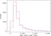 |
Fig. 1 Histogram of the amplitudes of sine curves fitted to the blue (dotted line) and red (solid line) light curve of η Cen (pre-whitened for the circumstellar 1.556 c/d variation). The frequency range is 1 c/d to 8 c/d with a step of 0.001 c/d. |
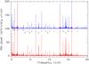 |
Fig. 2 AOV spectra of η Cen; the spectrum for the blue data is vertically offset. Because the orbital frequencies of the two satellites are very similar, the AOV spectra look similar as well, and the two spectra also illustrate the window function. The orbital frequency, fo, at ~14.4 c/d and its subharmonics are indicated by triangles, the 1.5562 c/d Štefl frequency and its harmonics and subharmonics by circles, and features due to combinations of the two by crosses. For stellar pulsations, fi, which typically have amplitudes more than an order of magnitude smaller than the Štefl frequency, fo − fi are the strongest aliases. For fi<fo/ 2 (~7.2 c/d), genuine frequencies and aliases with fo do not overlap. Since the Nyquist frequency is about fo/2, the range below it, fi<fo/2, are only contaminated by orbital aliases. |
Time-series analyses (TSA) in the range 0–20 c/d were carried out with the ESO-MIDAS (Banse 2003) context TSA, using the Analysis of Variance (AOV; Schwarzenberg-Czerny 1989) method. For comparison, conventional power spectra were also calculated. There were no great differences between the results.
Some periodic large-amplitude variations as described below for the two stars had to be removed to enable searches for weaker variations. This pre-whitening was performed by folding the data with the period in question, binning them to 0.02 in phase, and subtracting from each data point the average value of its home bin.
For a first overview of the data properties as described above, sine curves were fit at every frequency between 1 and 8 c/d with a step of 0.001 c/d. From the histogram of the fit semi-amplitudes (cf. Fig. 1), an initial quantitative indicator of the significance threshold for periodic variations can be deduced. If it is required that for an AOV feature to be considered significant its strength exceed that at the peak of the histogram plus three times the σ of the distribution, thresholds for the blue and red data of η Cen are 4.0 mmag and 3.6 mmag, respectively, in the range 1–8 c/d. The corresponding values for μ Cen are 3.3 mmag and 6.4 mmag. Analysis of constant, or nearly constant, Be stars shows (Baade et al., in prep.) that such estimates of the performance of BRITE-Constellation are overly conservative. But in μ and η Cen stellar noise also increases the detection thresholds.
For lower-amplitude variations, the frequently adopted method of recursive pre-whitening was not applied. This is possible because the strongest aliases, fo − fi, of intrinsic frequencies fi arise from the orbital frequency fo ≈ 14.4 c/d, which is analogous to 1 c/d in ground-based data. In BRITE data, 1-c/d aliases are mostly weak but not completely absent as a result of the daily variations of the solar illumination. In Fig. 2 they are not visible. For frequencies fi<fo/ 2, aliases of fo cannot be confused with the intrinsic frequencies fi (this relation is illustrated in Fig. 2). It is, then, convenient that the effective Nyquist frequency is fo/2 (there is mostly one data point per orbit) and the bulk of pulsation frequencies of Be stars occur in the range 0.5–10 c/d.
Every AOV feature that by its strength relative to its surroundings seemed to be possibly significant was checked by fitting a sine curve with the respective frequency. The analysis of the results suggested as an empirical (necessary but not sufficient) criterion that at least two of fi/2, fo − fi, and fo + fi should be clearly present in the AOV spectrum for fi to be considered significant. This criterion provides a stronger filter than an analysis of single AOV features alone. In a first step, searches for frequencies were also carried out in the product of the blue and red AOV spectra, which has a higher contrast. This method is very effective, but has the drawback of weakening the signature of low-amplitude variations and those with strong color dependencies.
The final results stated in the text and in Table 5 were obtained by fitting sine curves, starting with the frequencies found by AOV.
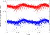 |
Fig. 3 Variability of η Cen with the 1.5562 c/d frequency (top: red passband, bottom: blue passband; phase zero point is arbitrary). In both light curves, note the deviation from sinusoidality and the non-random distribution of “outliers”, which are probably related to the mass-loss process and are not of instrumental origin. |
Frequencies below about 1 c/d pose a challenge because this range includes slow nonperiodic stellar variations such as outbursts, beat or similar phenomena related to higher frequencies, and possible instrumental drifts.
In summary, frequencies between 1 c/d and 8 c/d can be determined with high confidence. Analyses were performed using real as well as synthetic data in this frequency range of constant stars and very low-amplitude variables of comparable brightness. They showed (Baade et al., in prep.; see also Pigulski et al. 2016) that the above methods can reliably detect BRITE variables with amplitudes down to 0.5 mmag. (Here and throughout the remaining paper, all amplitudes correspond to the amplitude of a sine function, i.e., are semi-amplitudes, unless stated otherwise.)
5. Results
5.1. η Cen
The AOV spectrum (Fig. 2) is dominated by the Štefl variability with 1.5562 ± 0.0001 c/d and its aliases, some of which are stronger than the AOV line due to the satellites’ orbital frequency. Because of the very large amplitude (see Fig. 3), no other features were detectable with satisfactory confidence. Therefore, the 1.56-c/d variability was removed by pre-whitening.
Considering the power of the subtracted variability (blue amplitude: 22.8 mmag; red amplitude 20.6 mmag), the remaining peak-to-peak range was unexpectedly large (>200 mmag in the blue and >150 mmag in the red passband). To a good part, this is due to another strong but much slower variability with a frequency of 0.034 c/d (Fig. 4).
This 0.034-c/d signal was also subtracted, but the remaining variability was still large. AOV period searches found rapid variations with frequencies 1.732 and 1.767 c/d. The light curves are presented in Figs. 5 and 6. While the two corresponding AOV features seem to be relatively isolated (Fig. 7), most of the other frequencies come in groups (Sect. 5.3; Figs. 7 and 12). In Table 5 only the frequencies with the largest amplitude in their respective group are included.
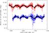 |
Fig. 4 Light curve (red: +; blue: ×, vertically offset by 0.15 mag) of η Cen after pre-whitening for the 1.5562 c/d Štefl frequency (without this pre-whitening, the structure of the light curve is extremely similar). Overplotted are fits with the frequency, 0.034 c/d, which corresponds to the difference between the 1.732 c/d and 1.767 c/d variations. Note the apparent outburst around day −160 (a second one may have occurred at day −245) and the enhanced scatter near extrema and especially minima. The phase of the blue variability may be slightly different from the red one. In view of the additional ephemeral variations, this is not considered to be significantly established. |
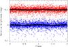 |
Fig. 5 Variability of η Cen with the 1.732-c/d frequency. The red-channel data are plotted at the top, blue data at the bottom. The signals from the 1.5562- and 0.034-c/d variations have been subtracted. A sine curve fitted with the 1.732-c/d frequency is overplotted. |
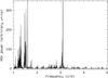 |
Fig. 7 Product of the AOV spectra (after pre-whitening for 1.5561 and 0.034 c/d) of the blue and red passband. Note the occurrence of frequency groups and the relative isolation of the peaks at 1.732 and 1.767 c/d. |
Inspired by the (spectroscopic) case of μ Cen, a relation of the 0.034-c/d variation to higher frequencies was searched for and quickly found. To within the errors, 0.034 c/d is the difference between the two frequencies of 1.732 c/d and 1.767 c/d. But the light curve does  exhibit a beat pattern (which in view of the low amplitudes and the presence of larger-amplitude variations is not expected). Instead, the low-frequency variability is very well reproduced by a sine curve with a frequency corresponding to the difference between the two 1.7-c/d frequencies. With 15 mmag, the amplitude of the 0.034-c/d variations is about five times as larger than either of the two higher frequencies (Table 5).
Another interesting finding is that the light-curve minima show somewhat more scatter than the maxima. Moreover, this scatter seems to vary from minimum to minimum. Some of these anomalies have event-like character (Fig. 4).
Because the 1.56-c/d Štefl frequency belongs to some extra-photospheric process, its properties were examined in more detail, and its value and amplitude were derived from sine fits in a sliding window of three days’ width. This window covers 4.5 cycles of the 1.5562-c/d variability so that the accuracy is reduced with respect to the full 135–150-d range. The analysis shows that the error margin stated above for the frequency (0.0001 c/d) is very misleading and only valid on average. As Fig. 8 (lower panel) suggests, the temporal variability of the frequency has an amplitude that is well over an order of magnitude larger: Only when averaged over many cycles is it roughly periodic. The amplitude is also variable and fluctuates between <15 and >35 mmag (Fig. 8, upper panel).
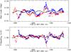 |
Fig. 8 Time dependence of the frequency (lower panel) and amplitude (upper panel) of the 1.5562-c/d variability in η Cen (red passband: +; blue passband: ×). Frequencies and amplitudes were determined as sliding averages over three-day intervals from sine fits. For comparison, the sine curve fitted to the light curve in Fig. 4 is overplotted with arbitrary scaling and vertical offset (note that the magnitude scale is inverted). |
The comparison of Fig. 8 with Fig. 4 reveals surprising correlations of both frequency and amplitude of the exo-photospheric Štefl variation with the star’s mean global brightness. But there does not seem to be a fixed phase relation, as can be deduced from the inclusion in Fig. 8 of the sine fit to the light curve in Fig. 4. Amplitude and frequency of the Štefl variability appear crudely anticorrelated but again with significant phase shifts. It is important to recall that the data in Fig. 8 were derived from sliding averages over three days, that is, about five cycles of the 1.5562 c/d variability. In other words, these figures do not contain information about variations with but of the Štefl frequency.
A frequency search over the range 1–7 c/d identified a few more frequencies well above the noise floor (see Table 5). All of them belong to frequency groups (Sect. 5.3) and are their respective strongest member. There are more frequency groups but their strongest features do not fulfill the adopted significance criteria.
5.2. μ Cen
The light curve of μ Cen (Fig. 9, see also Fig. 10) shows huge peak-to-peak amplitudes of about 200 and 250 mmag in the blue and the red passband, respectively. The timescales are much longer than 1 d, and several prominent features are visible in the AOV spectra below 0.15 c/d (Fig. 11), which practically prevent a meaningful search for higher frequencies because elementary confirmation from phase plots is impossible. Frequencies roughly shared (to within 0.005 c/d; these features are fairly broad) by both passbands include 0.025, 0.032, and 0.041 c/d. Because there is no such low-frequency power in observations with the same satellites of η Cen, it should be intrinsic to μ Cen. Folding the data with the corresponding hypothetical periods did not yield regularly repeating light curves. Of these frequencies, only 0.032 c/d may have a numerical relation, or more, to the spectroscopic beat frequencies of 0.018 and 0.034 c/d found by Rivinius et al. (1998c). Only contemporaneous spectroscopy could provide evidence.
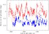 |
Fig. 9 The BRITE light curve of μ Cen (in instrumental, mean-subtracted magnitudes; red passband: +; blue passband: ×, vertically offset by 0.15 mag). |
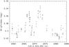 |
Fig. 10 The Strömgren b light curve of μ Cen as measured by Cuypers et al. (1989). |
In a next step, the AOV peaks below 0.15 c/d were recursively removed by pre-whitening. The noise level was reached with fewer than ten iterations. The remaining variations in magnitude were still ±50 mmag. This is very much higher than the instrumental noise and exceeds typical photometric amplitudes of nonradial pulsations in Be stars by an order of magnitude. Nevertheless, a detailed AOV analysis of the pre-whitened BRITE data did not identify a single significant candidate frequency in the range 1–7 c/d. This may be indicative that much of the residual ±50-mmag variability results from (circum-)stellar noise.
5.3. Frequency groups
The first Be star with identified groups of frequencies was μ Cen (Rivinius et al. 1998c). They consist of coherent (at least those showing beat processes) stellar eigenfrequencies, four around 2.0 c/d and two near 3.6 c/d. Limited sensitivity may well have prevented the detection of more frequencies in each group. There are no obvious inter-group relations. To distinguish these μ Cen-style frequency groups from the groups described below, they will be called Type I frequency groups.
In the AOV spectrum of η Cen, numerous spikes (“grass”) occur close to the 1.56-c/d Štefl frequency. Similar but weaker features can be found around 3.1 c/d. They are not direct harmonics of any individual feature near 1.56 c/d so that one might rather speak of “group harmonics”. Figures 7 and 12 give an overview of these Type II frequency groups in η Cen. They also show further tufts of grass, mainly shortward of 1.55 and 3.1 c/d (see Table 5 for more examples). Because it is based on data strings of no more than three days, Fig. 13 cannot resolve the Type II frequency groups around 1.2 and 1.55 c/d in η Cen into discrete AOV features. But there are major redistributions with time of the total power. The high structural similarity of the blue- and the red-passband diagrams in Fig. 13 confirms in a more encompassing way that this noise is intrinsic to η Cen and not instrumental.
A probably related result is that although many of the AOV spikes of frequency-group members are stronger than those of the 1.7-c/d frequencies, they do not pass the simple empirical significance check described in Sect. 4.1.
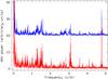 |
Fig. 12 Blue (top) and red (bottom) AOV spectra of η Cen after pre-whitening for the 1.5562 c/d Štefl frequency; see also Fig. 2. Note the numerous features (“grass”) around 1.55 and 3.1 c/d, but also below both frequency regions. The complex close to 4.8 c/d corresponds to one-third of the satellites’ orbital frequency (fo/ 3). Compare this figure also to Fig. 2. |
Several mechanisms are conceivable that could lead to frequency patterns that appear similar to this description of Type II frequency groups but actually are spurious. They were tested and eliminated one by one.
-
There could be instrumental noise. But simultaneous blue and red data obtained with different satellites show the same general phenomenon, while the cross-color match of individual features is poor. At the same time, the AOV spectra of μ Cen of data extracted from the same CCD images do not show similar features at the frequencies in question.
-
Pre-whitening with an incorrect (not genuine) frequency can introduce noise, the 1.556-c/d frequency is in the range concerned, and it is variable so that subtraction of a constant frequency is necessarily imperfect. But the features are visible before pre-whitening, and using different trial frequencies did not alter the nature of the frequency groups.
-
Deviations from sinusoidality can introduce artifacts during pre-whitening. But the pre-whitening procedure used does not make any assumptions about the shape of the variation.
-
Phase jumps due to outbursts can cause single frequencies to appear multiple. But: the other variabilities show no evidence of such jumps.
Because the AOV spectra of μ Cen are more “populous”, it is not obvious whether or not Type II frequency groups exist in this star as well. The best candidate appears around 3.4 c/d.
6. Analysis of the results
Be stars differ from other pulsating early-type stars in that, as pulsators, they are players but in addition also produce their own stages in the form of the circumstellar disks, which may echo the stars’ activity. This adds pitfalls to the analysis but also offers additional diagnostics. It is vital to not lose track of this duality. Extensive model calculations by Haubois et al. (2012) provide a very useful illumination of the photometric response to varying amounts of circumstellar matter as seen at different inclination angles.
6.1. η Cen
The photometric variability of η Cen contains major circumstellar components:
-
The ±3% variation of the frequency with the highest amplitude, 1.56 c/d (Fig. 8, lower panel), is not plausibly reconcilable with stellar pulsation although the mean value falls into the range of plausible g-modes. Since the frequency itself is slightly lower than the frequency of the strongest stellar pulsations, the classification as circumstellar Štefl frequency is confirmed.
-
The 0.034-c/d phased light curve shows noise beyond photon statistics and with subtle asymmetry: During minima it is slightly larger than during maxima. Because η Cen exhibits weak shell-star signatures (Rivinius et al. 2006) and is observed nearly through the plane of the disk, this probably means that matter is elevated above the photosphere and injected into the disk, where it removes light from the line of sight. This is shown in Fig. 4. In other stars, sudden increases in photometric noise have been observed to precede major brightenings (e.g., Huat et al. 2009).
-
Figure 4 also suggests that there was a discrete event in both passbands around day −160 and possibly a second one near day −245.
-
In addition to outbursts, regularly varying amounts of near-stellar matter in the disk could reprocess the stellar light and make part of it detectable along the line of sight. This would imply that the 0.034-c/d variation drives a quasi-permanent base mass loss.
-
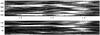
Fig. 13 Time-frequency diagram (bottom image: blue passband; top image: red passband) of the Type II frequency group around 1.55 c/d in η Cen, after pre-whitening for the 1.5562 c/d frequency. AOV spectra with a sampling of 0.0005 c/d were calculated over 3 d sliding averages. The frequency interval shown (abscissa) is 1.1–1.7 c/d. For both sub-images the AOV power (white is highest) was separately normalized to the respective mean power to facilitate comparison. The ordinates (in days) have arbitrary zero points. The two data strings have different starting dates but end at about the same time (cf. Fig. 4).
Similar to the 1.56-c/d peak, many of the other stronger peaks in the AOV spectrum are surrounded by numerous additional features forming a group (Sect. 5.3; Figs. 7 and 12).
Based on the photometry alone, the two frequencies near 1.7 c/d are only marginal detections. But the presence of the same frequencies in the Heros spectroscopy, which identified them as NRP modes (Sect. 6.5.1), clearly boosts them to significance. The agreement of the difference between these two frequencies and the 0.034-c/d variation suggests that all three are linked. If so (Sect. 7.4 resumes and completes this discussion), the regularity of the mean 0.034-c/d light curve indicates that the 1.7-c/d frequencies have a better phase coherence than the 1.5562-c/d Štefl frequency. The slow variability shown in Fig. 4 extends over 250 cycles of the 1.7-c/d variations. Frequency noise at the 3% level of the 1.7-c/d pulsations would not let the 0.034 c/d light curve repeat as well as it actually does.
It is interesting to note that the amplitudes of the two 1.7-c/d variations are only 2–3 mmag while the slow 0.034 c/d variation reaches nearly 15 mmag, which is about three times as much as the amplitude sum of the two fast variations (see Table 5).
If the 0.034-c/d variation does result from the interaction of two NRP modes, they would also become the root cause of the remainder of this complicated variability pattern: The individual cycles of the 0.034-c/d light curve (Fig. 4) and even the residuals from the mean amplitude are very well matched by the variability of the Štefl frequency and its amplitude. This suggests a fairly tight coupling between this pulsation-related process and the circumstellar Štefl process. But the large phase wiggles require the coupling to be quite elastic.
6.2. μ Cen
A particularly strong illustration of the need to take into account circumstellar variability is provided by this star. The combination of long timescale and very large amplitude of the dominant photometric variability makes the disk a much better candidate for the origin of this variation than the star. The variability is not due to a variable flux from the star. Instead, the varying amount of recently ejected matter in the near-stellar part of the disk reprocesses the presumably just very slightly intrinsically variable stellar flux and redirects part of it to the observer’s line of sight. Because the inclination angle is low (~20 deg; Rivinius et al. 2001), the effect is very pronounced (Haubois et al. 2012) and the amount of extra light provides a crude measure of the amount of extra near-stellar matter.
If μ Cen possesses any short-period low-amplitude variability, it would be difficult to detect against the flash lights of the large circumstellar activity. This parasitic light may be powered off by the temporary dispersal of the disk (cf. Peters 1986; Baade et al. 1988). However, what then becomes visible may not be representative of the active phases.
6.3. Frequency groups
By definition, Type I frequency groups consist of stellar NRP modes alone, and μ Cen is the first member of this class. It remains to be seen whether this class will continue to be so elusive. This photometric study did not identify any Type I group in either star (the two 1.7-c/d frequencies in η Cen do not seem to qualify as a group).
Because of their proximity in η Cen to the demonstratedly circumstellar Štefl frequency, Type II frequency groups may also be rooted in the near-photospheric environment. The drifting power in Fig. 13 reinforces this conclusion quite strongly (Sect. 7.4). Circumstellar processes are not expected to be strictly periodic, they must be intrinsically noisy, and there will be nonlinearities that lead to higher-frequency components. This is a good description of the “grass” close to the Štefl frequencies and of the group harmonics seen in BRITE AOV spectra of η Cen. Paper II elaborates on the appearance and nature of Type II frequency groups in much additional detail.
Neither the definitions of Types I and II nor the proposed explanation as stellar and circumstellar exclude the possibility that a star has frequency groups of both types.
6.4. Comparison of BRITE and earlier ground-based photometry
The following subsections discuss selected earlier observations. For both stars, a more complete overview and critical evaluation is provided by Rivinius et al. (2003).
6.4.1. η Cen
Because of its very large amplitude, the 1.56-c/d variation was detected by everyone with adequate data (e.g., Cuypers et al. 1989; Štefl et al. 1995). However, the phase instability sometimes made subharmonics look like a better match to the observations, causing some observers to conclude that this variability of η Cen is due to some co-rotating structures. The 0.52-c/d variant in particular was refuted by Rivinius et al. (2003), which is confirmed by the BRITE observations.
The amplitude of the 0.034-c/d light curve is only slightly lower (15 mmag vs. 20 mmag). But the timescale of a month means that ground-based observations cannot detect it.
6.4.2. μ Cen
Cuypers et al. (1989) published the only major photometric dataset of μ Cen obtained from the ground (Fig. 10). The light curve with frequency 0.476 c/d derived by these authors had a rather extreme, ragged shape, and is not at all supported by the BRITE observations.
This work and that of Cuypers et al. (1989) agree that the photometric variability does not contain any significant trace of the periods found in the long series of Heros spectra (Rivinius et al. 1998c). The strong signal can rather be thought of as some circumstellar light pollution. It is, therefore, a curious footnote that the photometry by Cuypers et al. (1989) – along with combined low- and high-order line-profile variability (Baade 1984) – provided the incentive to add μ Cen to the Heros target list, which resulted in the discovery of the most complex spectroscopic pulsation pattern found to date in any Be star (Rivinius et al. 1998c).
The comparison of Figs. 9 and 10 suggests that over as much as 27 yr (about 20 000 half-day pulsation cycles), the overall character of the photometric variability of μ Cen has not changed.
6.5. Comparison of BRITE photometry with earlier spectroscopy
6.5.1. η Cen
Rivinius et al. (2003) detected frequencies of 1.56 c/d, 1.73 c/d, and 1.77 c/d. The match with BRITE is excellent – even after almost two decades. Rivinius et al. (2003) identified the possibility that the beating of the two most rapid variations could lead to outbursts. But the series of spectra available to them was not sufficient to conclude this with acceptable confidence.
BRITE photometry alone does not provide any direct insights into the nature of the pulsations and, therefore, depends on spectroscopic support. Rivinius et al. (2003) found the line-profile variability associated with 1.73 c/d to be of the same type as in almost all other bright Be stars and attributed it to nonradial ℓ = m = + 2g-modes. In a later re-analysis of the Heros spectra, Zaech & Rivinius (unpublished) confirmed that both 1.7-c/d variations belong to this type.
The MiMeS project studied 85 Be stars (Wade et al. 2014b). In none of them was a large-scale magnetic field found. η Cen was not included in the sample but it was observed by ESPaDOnS (1×) and HARPSpol (9×). After careful reduction, the 9 measurements with HARPSpol (Piskunov et al. 2011) on 30 April 2014 were coadded and mean Least-Squares Deconvolved (LSD; Donati et al. 1997) profiles were extracted for the unpolarized (Stokes I), the circular polarized (Stokes V) and diagnostic null profiles. The longitudinal magnetic field measured from the LSD profile (9 ± 17 G; Wade et al. 2014b) provided no evidence of a magnetic detection. However, a marginal detection was established based on χ2 statistics (Donati et al. 1992) due to a series of pixels between about −50 and 200 km s-1 (the unpolarized LSD profile spans a velocity range between −400 km s-1 to 330 km s-1) that have signal outside of the error bars. This test computes the false-alarm probability (FAP) that measures the probability that the observed V signal inside the line profile differs from a null signal. In this case, there is sufficient signal in this line such that the FAP is low enough to consider this a marginal detection (10-6< FAP < 10-4). That is, the hypothesis that the line profile can be explained entirely by noise marginally disagrees with the observation. Since no excess or similar signal is found in the null profile, the feature seen is probably not instrumental.
Only additional observations can remove the attribute “marginal detection”. It is hoped that the ongoing BRITE spectropolarimetric survey (Neiner & Lèbre 2014) can achieve this among the ~600 targets to be observed brighter than V = 4 mag. The survey data taking is expected to be completed in the first half of 2016.
6.5.2. μ Cen
The analysis methods described above did not return a single one of the six spectroscopic frequencies (four of them near 2 c/d and two near 3.6 c/d) found by Rivinius et al. (1998c) and classified as ℓ = m = + 2g-modes. Therefore, a special “targeted” search for these frequencies was performed in the BRITE data. Weak AOV features occur at 1.991 and 2.027 c/d. The three strongest spectroscopic variations found by Rivinius et al. have frequencies of 1.988, 1.970, and 2.022 c/d. That is, at least the second strongest spectroscopic variation has no BRITE counter part.
μ Cen was observed with ESPaDOns on 24 February 2010 as part of the MiMeS project (Wade et al. 2014b). A new reduction of the data confirmed the non-detection at a level of Bz = 9 ± 12 G, which is also consistent with the results from the χ2 statistics.
Finally, not even a targeted search could detect the Štefl frequency at 1.61 c/d (Rivinius et al. 2003) in the red passband. In the blue AOV spectrum, a spike at 1.615 c/d is nearly the highest peak in what might be a Type II frequency group (or a high-frequency artifact caused by the large-amplitude slow variations).
7. Discussion
7.1. Synopsis of the variabilities of η and μ Cen
Table 6 juxtaposes a number of properties of η and μ Cen. At a first glance, the spectroscopic and photometric appearances of their pulsations seem confusing, if not contradictory. However, consideration of the difference in inclination angle reveals simple and well-known systematics:
-
η Cen
shows weak shell-star properties. This equator-on perspective favors the photometric detection of quadrupole modes, and freshly ejected matter re-directs relatively little light into the line of sight.
-
μCen
is viewed at a small inclination angle, which facilitates the detection of the latitudinal component of the horizontal g-mode velocity field (Rivinius et al. 2003). In photometry, much of the equatorially concentrated light variation (quadrupole modes) is lost to azimuthal averaging. Instead, the processing of radiation by regularly newly ejected matter close to the star leads to a huge photometric signal that outshines everything else.
Both stars suffer enhanced mass loss that is driven by a slow process assembled from two much more rapid nonradial pulsations. Because of the nearly edge-on perspective of η Cen, the variability is manifested in small fadings of this star, in contrast to μ Cen.
A Štefl frequency is present in the series of Heros spectra of both stars. But BRITE only found that of η Cen, at a considerable amplitude. This particular difference will be addressed in Sect. 7.5. The other difference lies in the degree of their persistence. In η Cen the Štefl frequency is quasi-permanent while in μ Cen its presence is coupled to enhanced line emission and the phase of the pulsational beat process. This could mean that the mass-loss process in η Cen is always active, but is occasionally enhanced at extrema of the slow 0.034-c/d variation.
7.2. Comparison to Kepler and CoRoT observationsof Be stars
It is of obvious interest to compare the BRITE observations of η and μ Cen to photometry of Be stars obtained with other satellites. For this purpose, the following considers the description by Kurtz et al. (2015) of Kepler observations of the late-type (B8) B and probable Be star KIC 11971405 and the behavior described by Huat et al. (2009) of HD 49330 (B0.5 IVe) during an outburst as seen by CoRoT.
The power spectra of both stars exhibit frequency groups. Balona et al. (2011) were among the first to ask whether such structures arise from rapid rotation and might even be characteristic of Be stars. Kurtz et al. (2015) concluded that frequency groups in Be, SPB, and γ Dor stars can be explained by simple linear combinations of relatively few g-mode frequencies. For the explanation of outbursts of Be stars, they adopted the same qualitative scheme as first developed by Rivinius et al. (1998a), namely NRP beating. This was significantly refined by Kee et al. (2014).
The appearance of the frequency groups is different during quiescence and outbursts. Both Huat et al. (2009) and Kurtz et al. (2015) suggested that during outbursts of Be stars a large number of pulsation modes flare up and drive the mass loss (see also Walker et al. 2005,for HD 163868). Because no physical explanation is given as to what would trigger such avalanches of pulsations, it is worthwhile searching for alternative descriptions of this behavior.
The BRITE photometry of η and μ Cen does offer an alternative view of the frequency groups seen by CoRoT and Kepler (and by MOST – Walker et al. 2005) if they also belong to Type II. Because of the natural circumstellar noise, this interpretation would require much less explanatory extrapolation into the unknown. A possibly important commonality is that the frequency groups in HD 49330 (~3 c/d and ~1.5 c/d) and KIC 11971405 (~4 c/d and ~2 c/d) as well as HD 163868 (~3.4 c/d and ~1.7 c/d) are crudely consistent with the description of 2:1 group harmonics. CoRoT and Kepler were more sensitive than BRITE is. Therefore, they do not see only a few blades of grass in their power spectra, but may observe a whole “prairie” springing up during outbursts of Be stars (see Paper II).
7.3. Modulations with azimuth
Because the stellar rotation frequencies are of the order of 70% or more of the Keplerian frequencies (Sect. 2.3) while the errors of both are well above 20%, the values of these frequencies are not suitable to determine the location of the Štefl process beyond confirming it to lie in the star-to-disk transition region.
Table 1 suggests that Štefl frequencies occur at about one-half of the maximal Kepler frequency. At the same time, the associated velocities are above equatorial velocities, which typically reach or exceed 70% of the critical velocity. This apparent (weak) contradiction may be resolved if the azimuthal period of the structures is a fraction of 360 deg. If the fraction is an integer, j, as in nonradial pulsations, j = 2 is a good guess. Because Štefl variations are not strictly periodic, j does not have to be an integer. But it simplifies the discussion to make such an initial assumption. In η Cen, the Štefl frequency is closely tied to the 0.034-c/d process, which involves a stellar quadrupole mode. Therefore, j = m = 2 is a good starting assumption also on this ground.
7.4. Nature of the 0.034-c/d variation in η Cen
Because of its sinusoidal shape, the 0.034-c/d variability of η Cen is the most unexpected discovery made by the observations with BRITE. Owing to its relation to mass loss, it is probably the signature of η Cen’s inner (mass-loss) engine. But the design of this engine remains enigmatic, and it may still be without precedence in Be stars. Therefore, the following sections aim at constraining its nature by exploring four very different hypotheses for its explanation.
First hypothesis: orbital variability in a binary system
In a binary system, a sinusoidal light curve can result from the distortion of two nearly identical stars. In this case, the orbital period would be twice 29.4 d, and the separation of two 9-M⊙ stars would amount to about 165 R⊙. This large separation would invalidate the hypothesis of tidal distortion. For a cool and large companion, 29.4 d could be the orbital period. But the separation would be too large for reflected light from the primary B star to have the observed amplitude. The absence of any extended constant parts of the light curve basically rules out partial eclipses.
Second hypothesis: companion-star-induced global disk oscillations
In binaries with a separation of about 0.5 au or more, eclipses may well not occur. However, if a companion is not too close to prevent the formation of a sizeable disk with Be star-typical line emission, it may induce global disk oscillations. The associated density waves carry a significant photometric signal (Panoglou et al. 2016), which in disks viewed pole-on can reach 100 mmag for strongly ellipical orbits. In η Cen, the sinusoidal variation would probably imply a fairly circular orbit and a very regular oscillation pattern. In some (but not all) Be binaries, V/R variations of emission lines track the orbital phase (Štefl et al. 2007). Because of slow large-amplitude variations in the strength and overall structure of the emission lines, the Heros spectra could not be used to search for periodoic V/R variability. However, this softer version of the binary hypothesis still faces the objection that matching radial-velocity variations were not discovered by Rivinius et al. (2003) and Rivinius et al. (2006). A low-mass sdO companion (see Rivinius et al. 2012 and Koubský et al. 2012 for the latest candidates added to the still very short list) might go unnoticed in radial-velocity data but would often reveal itself through He II 468.6 line mission from the region of the disk closest to it. The Heros spectra do not show this feature.
Third hypothesis: coupled nonradial pulsation modes
There is no known mechanism that would work with a single frequency of 0.034 c/d in the atmospheres of single early-type stars. However, the identity, to within the errors, of 0.034 c/d to the difference between the two short frequencies at 1.732 and 1.764 c/d is reminiscent of what in other stars is called a combination frequency. In the case of η Cen, it would be the difference between two pulsation frequencies. But frequency sums occur as well. The abundance of sums and differences is differently biased in different stars but the reason is not known. Wu (2001), Balona (2012), and Kurtz et al. (2015) discussed the amplitudes of combination frequencies in white dwarfs, δ Scuti stars, and γ Dor / SPB / Be stars, respectively. Kurtz et al. concluded that nonlinear mode coupling can give combination frequencies of g-modes a higher photometric amplitude than the parent frequencies. In their analysis, this results largely from the coupling of high-order modes to form low-order variations, which are less affected by cancellation effects across the stellar disk. But in η Cen the assumed parent modes are quadrupole modes, and the amplification factor would be huge with three times the sum of the two 1.7-c/d variations. To include these facts would probably require a siginificant extension of the notion of combination frequencies.
Fourth hypothesis: circumstellar activity
It is at least an odd coincidence that not only the two stellar 1.7-c/d frequencies differ by 0.034 c/d but the circumstellar 1.5661-c/d frequency also differs by this amount from its two strongest neighboring peaks in the AOV spectra (Table 5). As Fig. 8 has illustrated, the 1.5562-c/d frequency is not constant but varies by more than 0.034 c/d. On this basis, one would dismiss the agreement as an oddity, especially since the entire frequency group of which 1.5562 c/d is the strongest member by far, does not seem to be phase coherent either, see Fig. 13. However, if the three frequencies near 1.56 c/d shifted around in the same fashion, this argument could be invalid. In fact, the said two companion peaks to 1.5562 c/d are variable in position. Although the measuring errors are much larger than for the central peak, their variability is similar. But the amplitudes of the frequency variations are nearly twice as large as the one of the 1.5562-c/d frequency. This appears significant since the two substantially weaker stellar 1.7-c/d variations show much less scatter, which is consistent with the hypothesis of constant frequencies.
Conclusion
The ecplising-binary hypothesis can be safely excluded. The first and the second one are weakened by the lack of radial-velocity variations. These first two and the fourth hypothesis have in common that they do not offer a connection between the 0.034-c/d variability and the equally large difference in frequency between the two 1.7-c/d stellar pulsations. If such an explanation is required, a coupling of the two pulsation modes is the only useful ansatz among the four options considered, although it may be of a rather different nature than combination frequencies in other g-mode pulsators.
The third hypothesis alone seeks the explanation within the star instead of in the disk. Therefore, a strong argument in support of it derives from the association of the 0.034-c/d frequency with both mass loss and the variability of the circumstellar Štefl frequency. The cause of the mass loss must be in the photosphere or below it, and the strong response of the Štefl frequency to small outbursts that are synchronized with the 0.034-c/d variability is a manifestation of this causal connection.
For these reasons the discussion below only considers the hypothesis of coupled NRP modes even though it acknowledges that this choice for the explanation of the inner engine is not unequivocally forced by the available data.
7.5. Two mass-loss engines working in series
Since the discovery of Štefl frequencies, the evidence has been strong that they are closely related to the mass loss from Be stars and trace super-photospheric processes. The combination of Heros spectroscopy and BRITE photometry has established this firmly. Before BRITE there was some ambiguity as to whether the pulsation enables the Štefl frequency or whether the Štefl frequency is somehow the rhythm of the engine injecting mass into the circumstellar disk. The correlations of the variations of the frequency and the amplitude of the Štefl frequency (Fig. 8) with the probably pulsation-related 0.034-c/d variation found by BRITE in η Cen give convincing support to the former because otherwise the circumstellar Štefl process would have to be driving the stellar pulsation.
Moreover, the said ambiguity is not a conflict, and the available spectroscopy and photometry are not contradicted by the working hypothesis that both are true: the pulsations enable the Štefl frequency, which in a second stage of the mass-loss process feeds the disk. This two-stroke process consisting of an inner (pulsations) and an outer (Štefl process) mechanism that operates the mass-transfer from star to disk in η Cen is one particular realisation of the general two-engine concept.
7.5.1. Inner engine: interacting nonradial pulsation modes
η Cen was selected as a BRITE target because of indications of quasi-permanent mass loss and beating of two NRP modes (Rivinius et al. 2003) so that any physical connection between them could be identified and characterized. The actual chain found by BRITE is more complex than anticipated:
-
Two nonradial pulsation modes (1.7 c/d)
-
combine in an unknown fashion to a much slower variability (0.034 c/d)
-
which drives the mass loss (possibly dissipating more energy than the linear sum of the two modes)
-
and connects to the circumstellar Štefl process (1.56 c/d) that probably is the mechanism by which the matter organizes itself into circumstellar structures.
In μ Cen, no specific mode interaction has been inferred other than that outbursts repeat with the difference frequencies of several NRP modes. But there is no direct evidence of a beat phenomenon with its characteristic envelope describing the variation of the combined amplitude. It is not excluded that μ Cen is an η Cen analog, but more complicated because at least three frequencies are involved.
Examples of Be stars with light curves exhibiting a classical beat phenomenon can be seen in Fig. 16 of Martayan et al. (2007) and in Fig. 5 of Diago et al. (2008). But the authors did not report outbursts occurring with the beat frequencies of the four stars concerned, which are members of the open cluster NGC 330 in the Small Magellanic Cloud.
At the same time, the very bright and nearby examples 28 ω CMa and Achernar suggest that there ought to be many single-mode Be stars. They would have to function somewhat differently but with the same basic outcome, namely a decretion disk, and an explanation is needed for them.
For instance, if mass loss opens a valve through which pulsation energy leaks, the interaction between two NRP modes opens and closes this valve periodically. But in a single-mode pulsator it would stay open until the energy supply is temporarily exhausted and needs to be rebuilt. There is also the suggestion by Ando (1986) that nonradial g-modes can act as stellar core-to-surface carriers of angular momentum (see also Lee et al. 2014).
Alternatively, apparent single-mode pulsators with outburst repetition timescales of a decade like 28 ω CMa and Achernar may in reality be multimode pulsators with frequency separations of as little as 3 × 10⁻⁴ c/d. Existing ground-based observations do not have the necessary precision, and space data do not have enough time coverage to reject or confirm this hypothesis so that any new observational effort would require a long shot well into the next decade.
7.5.2. Outer engine: large-scale gas circulation flows
The outer engine is no less difficult to reverse-engineer because stars other than Be stars do not cast the matter they lose into a Keplerian disk and so cannot provide much guidance. Therefore, the following attempts to bootstrap the properties of the outer engine that regulates this process:
-
The outer engine is located in the transition region between star and disk because the Štefl frequencies are associated with superequatorial velocities.
-
It is fed by the inner engine, which is powered by low-order nonradial g-mode pulsation as discussed in Sect. 7.5.1.
-
The outer engine stops working when the inner engine (pulsation) does not deliver enough matter (and associated energy and angular momentum) to it.
-
Because of the appearance of the Štefl frequencies in spectral lines, the outer engine seems to be tied to the azimuthal modulation of the gas density just above the photosphere proper.
-
The Štefl frequency of μ Cen manifests itself in the spectroscopy, but not in the photometry. In η Cen, the Štefl frequency is revealed by both observing techniques. μ Cen is seen at a small inclination angle, while η Cen is viewed through its disk. Because the presumed outer engine is close, but not very close, to the star, this could mean that in η Cen there is an occultation process at work, and in μ Cen the outer engine is visible all the time.
-
The operating frequency of the outer engine (the Štefl frequency) is slightly lower than the frequency of the related pulsation.
-
This could imply that the azimuthal period of the density modulation is about the same as the period of the nonradial quadrupole modes typical of Be stars (Rivinius et al. 2003), namely 180 deg.
-
The operating frequency is not phase coherent but wobbles at the few-percent level.
-
As a result, the hypothesized regions of enhanced density do not have a stable azimuthal position but can drift by significant amounts.
-
This would disfavor stellar magnetic fields as the “anchor” of the density enhancements unless such magnetic fields also drift around. This agrees with the magnetic-field measurements mentioned above.
-
Maybe a simpler mechanism for the density modulation is dynamic: For instance, there could be large-scale circulation flows and the density be enhanced where the circulation velocities are lower or cause photometric variations in some other way. That is, the observed circumstellar variations are not caused by fixed lumps of orbiting matter, but by pile-ups in the flow. There are at least two ways by which this could work (if at all):
-
At the inner edge of gaseous Keplerian disks, there can be circulatory motions known as Rossby Wave Instability (Lovelace et al. 1999; Li et al. 2000). They might also provide the seed for the viscosity of the decretion disks of Be stars.
-
In the terrestrial atmosphere and all gaseous planets of the solar system, circulatory gas flows are observed that are related to Rossby waves. Of particular interest might be that these gas flows, which are driven by fast rotation and temperature differences, are linked to jet streams. See Oishi (1926) for the Earth, Simon-Miller et al. (2012) for Jupiter, Del Genio & Barbara (2012) for Saturn, and Kaspi et al. (2013) for Uranus and Neptune. That is, these are powerful, energetic processes. But note that not even in the solar system is the formation of jet streams fully understood (Baldwin et al. 2007).
-
-
In Fourier space, a Štefl frequency, which in η Cen is sitting amidst the Type II frequency group at 1.55 c/d, would only be the tip of an iceberg consisting of all the intrinsic noise and nonlinearities associated with the circulation process. Group harmonics will arise very naturally. Regardless of whether the circulation motions are in the outer stellar atmosphere or the inner disk, still images and movies of planetary atmospheres may provide some guidance as to what to search for. This is a very close match of the model-free description given above of the photometric Type II frequency groups in Be stars.
The innermost part of the disk would thus consist of spatially quasi-periodic gas circulation cells. They would owe their existence to one or more of (i) the rapid rotation of the central star; (ii) the large pole-to-equator temperature differences; (iii) the detachment process of the gas leaving the star (and, in Be stars, partly returning to it from a viscous disk); and (iv) the variation of the local mass-loss rate with stellar azimuth. The gas temporarily trapped in these cells could be supplied by stellar g-mode pulsation when the amplitude is large enough.
The above design of the outer engine was derived in a purely empirical way. It does not compete with the VDD model, but may rather supply it with inner boundary conditions. It also has major implications for the interface between inner and out engine.
7.5.3. Coupling two engines running at very different frequencies
Describing this interface is a challenge: Any model for the mass loss from Be stars must explain how, on the one hand, the variabilities with the NRPs (to be precise: the slow process linked to the pulsation) and Štefl frequencies can be so closely coupled and how, on the other hand, such a causal chain is not broken by the difference in the frequency. The difference in observed frequency may be related to the phase velocity of the NRP waves. However, not even the sign of the latter is clear: Rivinius et al. (2003) found retrograde modes to well describe their spectroscopic observations of two dozen Be stars. By contrast, theoretical models often prefer prograde modes, especially if they are “tasked” with supporting the star-to-disk angular-momentum transfer; see Kee et al. (2014) for a discussion.
But the frequency difference exists, and so does the mystery of two processes that are closely connected but operate at quite different frequencies. The mystery is probably extended by the fact that the Štefl frequencies seem to follow the pulsation frequencies over a range of at least a factor of >2 when all stars with available data are considered together (see Table 1). The concept of large-scale circulation motions can also deliver on this challenge. Because they seem to prevail only during phases of significant mass loss that feeds them, the matter participating in these motions is permanently replaced with new one. Therefore, the observed frequencies of these structures are like phase frequencies whereas the physical causality is maintained by the physical motions of the gas. In this way, a quadrupole mode can supply two huge eddies with matter, which nevertheless propagate with a different azimuthal velocity.
In the proposed context, it does not appear surprising that the amplitude of the Štefl frequency scales with residuals from the mean brightness: A stronger stellar action (mass loss) leads to a stronger circumstellar response. The variable phase relation suggests that the logical rope linking the two processes must be fairly elastic. The approximate anticorrelation between the Štefl frequency and its amplitude can be understood such that when the mass loss is higher, there is more matter close to the star, where orbital frequencies are higher. Such a change in frequency is nothing but a change in phase, so that the variable phase is also explained.
7.6. Other early-type stars
The above description places the circulation streams in the inner disk. But the available observations cannot rule out similar motions in the outer stellar atmosphere.
If there is an analogy between Be stars and the atmospheres of rocky as well as rapidly rotating gaseous planets, these cases would probably bracket other stars with significant rotation and extended atmospheres. The phenomenon that such a conjecture brings immediately to mind are the Discrete Absorption Components (DAC’s) in the UV wind lines of virtually all massive stars. Massa & Prinja (2015) have recently shown that they must arise at a location very close to the photosphere. At 15–20% of the stellar diameter, their footprints are quite large.
Radiatively driven winds are so extremely intrinsically unstable that a considerable variety of large-scale perturbations seem, in principle, capable of growing into DACs (Cranmer & Owocki 1996). The challenge is to explain the apparent semi-regular angular partition. Based on the analysis of ten O-type stars, Kaper et al. (1999) argued that the azimuthal period is often (but clearly not always) close to 180 deg. Magnetic fields might be too rigid, given the frequent large deviations from genuine periodicity. More importantly, MiMeS has found global magnetic fields in fewer than 10% of all early-type stars (Wade et al. 2014a). In a targeted search in 13 OB stars with prototypical DAC behavior, David-Uraz et al. (2014) did not detect dipolar magnetic fields in any of them. But DACs occur in virtually all luminous O stars (Howarth & Prinja 1989). Nonradial pulsations are perhaps similarly ubiquitous among stars with radiative winds so that their native angular periodicity makes them a stronger contender for the explanation of DACs than magnetic fields. However, low-order NRPss do not seem to be common in O-type stars (see, e.g., the examples of ζ Oph, ξ Per, and ζ Pup mentioned below).
Gas circulations in the transition region between photosphere and base of the wind might constitute a plausible alternative. But the mostly much lower temperature contrast between equator and poles than in Be stars, in which it is caused by the fast rotation and may even lead to significant equatorial convective motions, may not be able to channel enough energy into this process. Moreover, the much higher radiation pressure could inhibit such flows altogether.
Recently, Ramiaramanantsoa et al. (2014) reported on observations with the MOST satellite of the bright O star ξ Per (O7.5 III(n)((f))). There are several 1 mmag variations near 0.5 c/d, which is interpreted as twice the rotation frequency. Assuming that there are two roughly identical regions along the stellar circumference, Ramiaramanantsoa et al. (2014) attributed the photometric variability to photospheric spots. The best description found of the data is that the spots propagate at one and the same angular rate (that of the stellar rotation), but are relatively short lived with spots disappearing after a while and new ones developing. If the size of these spots is as large as inferred by Massa & Prinja (2015), their brightness contrast must be quite low.
It seems difficult to distinguish this photometric variability of ξ Per from the Štefl frequencies of η and μ Cen and α Eri: low-amplitude, roughly integer fraction of the rotational timescale (with rotational eclipses), and poor phase coherence. If this means that the phenomena are of the same nature, and if gas circulation cells are responsible for them, they would in ξ Per reside in the star because Be-star disks are neither known nor expected to develop around very hot and luminous stars. In agreement with this, ξ Per does not exhibit the very high noise associated with Štefl frequencies in Be stars. Another difference is that O stars do not seem to pulsate in low-order nonradial modes (and the higher-order pulsation does not appear to modulate the mass loss).
Another bright prototypical O star is ζ Pup (O4 If(n)p), albeit with above-average space and rotational velocities. BRITE has also observed this star. Ramiaramanantsoa et al. (in prep.) find that this star’s behavior is similar to that of ξ Per, but is more stable. The frequency of 0.56 c/d was also seen for nearly four years by SMEI (Howarth & Stevens 2014) and falls into a gray zone between rotation and pulsation. The proximity to the Sun of ξ Per and ζ Pup attracts the same argument as for μ (and now also η) Cen: There must be many more such stars.
If the facts put together in this subsection do belong together, any attempt of their explanation is faced with the combination of large spatial size, low photometric contrast, and high significance in velocity. Circulation flows seem capable of coping with such a challenge. In a study that has remained without follow-up by the hot-star community, Dowling & Spiegel (1990) have undertaken a first theoretical reconnaissance investigation of the properties of putative large-scale vorticities in rapidly rotating hot-star atmospheres. They concluded that the associated photometric contrast will be low because the vorticities are shallow and so have little flux-(de)focusing power. Dowling & Spiegel also considered that such vorticities may be related to the ubiquitous microturbulence invoked to explain excess line broadening. This is quite similar to the proposal by Lucy (1976), which, however, is based on multi-mode nonradial pulsation. The two explanations can probably co-exist (also with the convection-based model of Cantiello et al. 2009). But the empirical evidence of nonradial pulsation in early-type stars is mostly limited to few discrete modes (cf. ξ Per and ζ Pup). Vorticities may more readily lead to a continuum of motions.
7.7. Options for verification
Because of their velocity contrast, the hypothesized circulation regions in Be stars would probably have a small radial extent, just some fraction of the stellar radius. Such considerably sub-milliarcsec structures are too small for current optical and infrared interferometers, which, for observations of Be-star disks, often use the central stars as unresolved calibrators.
In shell stars, where the line of sight passes through the plane of the disk, the disk structure can also be probed by high-resolution spectroscopy. There is a seemingly unparalleled series of high-resolution spectra by Hanuschik & Vrancken (1996) of 48 Lib (B3 IVe-sh), which recorded the presence for a few months as well as the very rapid variability of multiple narrow absorption components in optical low-excitation shell lines. Because of its uniqueness it has not found an understanding based on a broad interest and discussion. Hanuschik and Vrancken offer as one explanation “higher-order, local distortions in the global spiral pattern” (referring to global disk oscillations as described by Okazaki 1991). It could just as well be the low-spatial frequency noise farther out in the disk of the circulation flows. That is, spectroscopy at high time and spectral resolution of shell stars could contribute to unraveling the Štefl process.
Of the available observables, polarization is probably the one most strongly focused on the conditions in the immediate vicinity of the central star as has been shown by Hayes & Guinan (1984), Guinan & Hayes (1984), and Carciofi et al. (2007). It could be useful to try to compare temporal power spectra of fast polarimetry with spatial power spectra of models of near-stellar disk structures.
Štefl frequencies were discovered in series of spectra of Be stars without strong shell-star characteristics. However, while the Heros spectra (Štefl et al. 1998) were sufficient for detection purposes, the detailed nature of the variability cannot be derived from them. The separation in radial velocity of the Štefl variability from much of the photospheric variability is an asset, but the contamination will still be large. This would make a new spectroscopic campaign quite expensive with uncertain outcome.
In photometric power spectra, the separation of Štefl and main pulsation frequencies is more favorable. In long time-series, the width of discrete pulsation frequencies will be negligible for the given purpose. If in addition the sampling is high, power spectra can be calculated in sliding time windows. This will unambiguously establish whether the “grass” in the power spectra of Be stars is or is not phase coherent, that is, whether it is rooted deep inside the star or grows in the star-disk transition region. The four-year Kepler database satisfies these requirements and forms the basis of Paper II, which also deploys wavelet analyses.
This reasoning ignores the possibility of stochastically excited pulsation modes (e.g., Neiner et al. 2012). It would be very valuable to secure spectra of the B-type stars observed by Kepler and other satellites that exhibit power spectra with particularly rich groups of transient spikes. If stars with such properties are mainly Be stars, the non-stellar origin of Type II frequency groups would be further strengthened. Such efforts should take into account the widespread volatility of Be-star disks and the emission lines forming in them.
One of the most promising follow-up projects should be the comparison of (equator-on) Be stars to very rapidly rotating B-type stars without disks and emission lines, so-called Bn stars. Thirty years ago, Penrod (1986) reported that only Be stars show low-order NRPs, while Bn stars – and many Be stars – pulsate in high nonradial-order modes. A possibly related observation (Waelkens 1990) is that with increasing rotational velocity the prevalent nonradial mode order, m, may also increase. Aerts & Waelkens (1993) pointed out that this may only be apparent because at higher rotation rates larger toroidal terms alter the velocity field of low-order modes. However, a comparison of Bn and equator-on Be stars may be less susceptible to such effects. Moreover, SPB stars have been added to the B-type stars with long-period, low-order g-modes, and some of them show relatively rapid, but not extreme, rotation (e.g., Daszyńska-Daszkiewicz et al. 2015). The triangle of Be, Bn, and SPB stars should provide for valuable intercomparisons. Moreover, Bn and SPB stars should be free of circumstellar noise and in this way contribute indirectly, by elimination, to understanding the latter.
8. Conclusions
The good agreement between BRITE photometry, Heros spectroscopy, and other observations taken up to more than two decades apart suggests that, for the combinability of observations of Be stars, high Fourier quality (sampling, resolution) is at least as important as proximity in time. This consistency deserves to be contrasted with the still widespread belief that Be stars behave in an erratic way. The latter is quite certainly true if their sometimes-complex variability is not properly captured by the observations, be it because of too sparse sampling or too short data strings or both. But insufficient data is not an intrinsic property of Be stars.
Thanks to the so enabled combination of BRITE photometry and Heros spectroscopy it is possible to take advantage of the fact that nature has been benign in orthogonalizing the Be problem: it can be separated into an inner and an outer engine. In addition to confirming this, the new BRITE data provide a more detailed view of the complex interface between the inner and outer Be-star engines. The Štefl frequencies seem to be the key element of this interface.
Contrary to stellar pulsations, the circumstellar Štefl frequencies exhibit substantial “deficiencies” in phase coherence and are accompanied by numerous other similarly deficient frequencies. If they are mistaken for stellar pulsations, they may be (incorrectly) interpreted as a large number of pulsation frequencies. The BRITE observations of η and μ Cen suggest that the complexity of the power spectra of Be stars does not lie in exotic variations of stellar pulsations that, if related to g-modes, are rooted deeply inside the star but rather in temporary circumstellar processes that are only quasi-periodic.
At the most elementary level, the variability of Be stars such as η and μ Cen may possibly be characterized by as few as three numbers: two stellar pulsation frequencies and a slightly lower circumstellar Štefl frequency. In addition, a formula is needed that describes how the two NRP modes join (or even amplify) their forces. The Štefl frequency is accompanied by a Type II frequency group and 2:1 group harmonics. The sometimes reported extreme multi-periodicity of Be stars during outbursts would be an illusion that is due to the noise of the circumstellar activity, for instance, in large gas-circulation flows. Its diagnostic value would not be diminished, however, but shift from asteroseismology to the hydrodynamics of the mass-loss process. The variations of the Štefl frequencies in value and amplitude seem to be good tracers of the mass supply from the star to the disk.
A still simpler variant would not require an interaction of two short-term variations. A single NRP mode energizes the outer mass-loss engine directly and supplies it with angular momentum from deep inside the star until its own energy supply is exhausted after some years.
The distinction made between multi- and single-mode pulsators among Be stars does not lead to a black-and-white picture: multi-mode pulsators like ζ Oph (O9.2 IVe) may show variable pulsation amplitudes and undergo outbursts, but do not exhibit any obvious signs of outbursts being related to some combination of the pulsations (Howarth et al. 2014). However, the frequencies of up to 7.2 c/d are mostly on the high side for low-order g-modes. Spectroscopic evidence is available for only some of the variations and indicative of medium m values. That is, ζ Oph does not contradict the interacting-modes paradigm, but may have more in common with the single-mode pulsators.
A valid concern about the rotation-plus-pulsation hypothesis for the mass-loss mechanism from Be stars can be deduced from the apparent dichotomy between early-type Be stars, which are invariably quite active, and Be stars of late spectral sub-classes, which often hardly display any activity at all (Rivinius et al. 2013b). This may be just a difference in amplitude: Star KIC 11971405 is of spectral type B8, but the precision photometry with Kepler (Kurtz et al. 2015) shows it to be pulsating and probably undergoing mass-loss events. Pulsations were also detected by BRITE in other late-type Be stars (Baade et al., in prep.).
If the coupling of NRP modes can release more energy than their simple linear combination, it could enable the formation of disks also around late-type Be stars with low NRP amplitudes. This could be helped by a fractional critical rotation that increases with decreasing mass (see Rivinius et al. 2013b, for a detailed discussion). Furthermore, Vieira et al. (2015) found that disks around late-type Be stars have much lower densities.
In the atmospheres of solar-system planets, jets are powered by rotation and temperature differences, in accretion disks Rossby waves with similar circulatory motions are predicted (Lovelace et al. 1999; Li et al. 2000), and Dowling & Spiegel (1990) discussed jets for hot-star atmospheres. That is, these circulation flows are significant power houses and could form part of the outer engine. If they do occur, their high-momentum end could also provide the physical basis for the mass-ejection process in the model of Kroll & Hanuschik (1997), which otherwise laid a promising foundation to a realistic reproduction of the disk variability of μ Cen following outbursts.
In summary, a cartoon inspired by η Cen of a Be star in outburst could look as follows:
-
A double wave is propagating along the stellar equator. It results from the temporary superposition of two or more nonradial quadrupole modes.
-
Nonlinear coupling at the difference frequency of the NRP modes leads to significant amplification beyond the amplitude sum of the parent frequencies.
-
At phases of maximal amplitude, outbursts are triggered.
-
The matter so propelled flows to, and is circulated through, two large eddies at the base of the disk. These eddies propagate at a different angular velocity than the stellar pulsation waves. It is the sum of the local Keplerian angular velocity and any phase velocity of the vortices and corresponds to the Štefl frequency. The latter is not constant because the vortices may move both radially and azimuthally.
-
Conservation of the total angular momentum limits the fraction of the matter that does reach orbital velocities to a small number. The rest loses angular momentum in a plethora of small eddies and eventually falls back to the star (cf. Okazaki et al. 2002; Rivinius et al. 2013a). These small circulation cells are the source of the noise seen during outbursts and may be the seed of the viscosity in the VDD model. It may be fitting that a first determination of the viscosity parameter in a Be disk yielded a rather high value (Carciofi et al. 2012).
Forthcoming papers in this BRITE string of the series will examine late-type Be stars and a comparison of Be and Bn stars. Studies of individual Be stars will include one of 27 and 28ω CMa (which are being observed by BRITE at the time of writing). They form a (nonphysical) couple of early-type Be stars very similar to η and μ Cen with one shell (27) and one high-inclination (28ω) star. In neither of them, multiple frequencies have been detected to date.
Acknowledgments
D.B. and T.R. dedicate this paper in gratitude to their long-term collaborator and friend Stanislav (Stan) Štefl (1955–2014), with whom this project had been planned like so many others before. The authors thank the BRITE operations staff for their untiring efforts to deliver data of the quality that enabled this investigation. They appreciate the permissions by Tahina Ramiaramanantsoa et al. to mention some early results of their ongoing work on ζ Pup. Coralie Neiner is thanked for the early communication of magnetic-field measurements with ESPaDOnS of η Cen. This research has made use of the SIMBAD database, operated at CDS, Strasbourg, France. This research has made use of NASA’s Astrophysics Data System. ACC acknowledges support from CNPq (grant number 307076/2012-1) and FAPESP (grant number 2015/16592-0). GH thanks the Polish NCN for support (grant 2011/01/B/ST9/05448). A.F.J.M. is grateful for financial aid from NSERC (Canada) and FRQNT (Quebec). A.P.i. acknowledges support from the Polish NCN grant No. 2011/03/B/ST9/02667. A.P.o. acknowledges support through NCN grant No. 2013/11/N/ST6/03051. G.A.W. acknowledges Discovery Grant support from the Natural Sciences and Engineering Research Council (NSERC) of Canada. The authors from Poland acknowledge assistance by BRITE PMN grant 2011/01/M/ST9/05914.
References
- Aerts, C., & Waelkens, C. 1993, A&A, 273, 135 [NASA ADS] [Google Scholar]
- Ando, H. 1986, A&A, 163, 97 [NASA ADS] [Google Scholar]
- Baade, D. 1982, A&A, 105, 65 [NASA ADS] [Google Scholar]
- Baade, D. 1984, A&A, 135, 101 [NASA ADS] [Google Scholar]
- Baade, D., Dachs, J., van de Weygaert, R., & Steeman, F. 1988, A&A, 198, 211 [NASA ADS] [Google Scholar]
- Baldwin, K. P., Rines, P. B., Huang, H. P., & McIntyre, M. E. 2007, Science, 315, 367 [CrossRef] [Google Scholar]
- Balona, L. A. 2012, MNRAS, 422, 1092 [NASA ADS] [CrossRef] [Google Scholar]
- Balona, L. A., Pigulski, A., Cat, P. D., et al. 2011, MNRAS, 413, 2403 [NASA ADS] [CrossRef] [Google Scholar]
- Banse, K. 2003, Information Handling in Astronomy – Historical Vistas, 285, 89 [Google Scholar]
- Bolton, C. T. 1982, in Be Stars, eds. M. Jaschek, & H.-G. Groth, IAU Symp., 98, 181 [Google Scholar]
- Cantiello, M., Langer, N., Brott, I., et al. 2009, A&A, 499, 279 [NASA ADS] [CrossRef] [EDP Sciences] [Google Scholar]
- Carciofi, A. C., Magalhães, A. M., Leister, N. V., Bjorkman, J. E., & Levenhagen, R. S. 2007, ApJ, 671, L49 [NASA ADS] [CrossRef] [Google Scholar]
- Carciofi, A. C., Bjorkman, J. E., Otero, S. A., et al. 2012, ApJ, 744, L15 [NASA ADS] [CrossRef] [Google Scholar]
- Cranmer, S. R., & Owocki, S. P. 1996, ApJ, 462, 469 [NASA ADS] [CrossRef] [Google Scholar]
- Cuypers, J., Balona, L. A., & Marang, F. 1989, A&AS, 81, 151 [Google Scholar]
- Daszyńska-Daszkiewicz, J., Dziembowski, W. A., Jerzykiewicz, M., & Handler, G. 2015, MNRAS, 446, 1438 [NASA ADS] [CrossRef] [Google Scholar]
- David-Uraz, A., Wade, G. A., Petit, V., et al. 2014, MNRAS, 444, 429 [NASA ADS] [CrossRef] [Google Scholar]
- Del Genio, A. D., & Barbara, J. M. 2012, Icarus, 219, 689 [NASA ADS] [CrossRef] [Google Scholar]
- Diago, P. D., Gutiérrez-Soto, J., Fabregat, J., & Martayan, C. 2008, A&A, 480, 179 [NASA ADS] [CrossRef] [EDP Sciences] [Google Scholar]
- Domiciano de Souza, A., Kervella, P., Moser Faes, D., et al. 2014, A&A, 569, A10 [NASA ADS] [CrossRef] [EDP Sciences] [Google Scholar]
- Donati, J.-F., Semel, M., Carter, B. D., Rees, D. E., & Collier Cameron, A. 1997, MNRAS, 291, 658 [NASA ADS] [CrossRef] [MathSciNet] [Google Scholar]
- Dowling, T. E., & Spiegel, E. A. 1990, Annals of the New York Academy of Sciences, 617, 190 [NASA ADS] [CrossRef] [Google Scholar]
- Ducati, J. R. 2002, VizieR Online Data Catalog: II/237 [Google Scholar]
- Goss, K. J. F., Karoff, C., Chaplin, W. J., Elsworth, Y., & Stevens, I. R. 2011, MNRAS, 411, 162 [NASA ADS] [CrossRef] [Google Scholar]
- Grady, C. A., Bjorkman, K. S., & Snow, T. P. 1987, ApJ, 320, 376 [NASA ADS] [CrossRef] [Google Scholar]
- Grady, C. A., Bjorkman, K. S., Snow, T. P., et al. 1989, ApJ, 339, 403 [NASA ADS] [CrossRef] [Google Scholar]
- Guinan, E. F., & Hayes, D. P. 1984, ApJ, 287, L39 [NASA ADS] [CrossRef] [Google Scholar]
- Hanuschik, R. W., & Vrancken, M. 1996, A&A, 312, L17 [NASA ADS] [Google Scholar]
- Haubois, X., Carciofi, A. C., Rivinius, T., Okazaki, A. T., & Bjorkman, J. E. 2012, ApJ, 756, 156 [NASA ADS] [CrossRef] [Google Scholar]
- Haubois, X., Mota, B. C., Carciofi, A. C., et al. 2014, ApJ, 785, 12 [Google Scholar]
- Hayes, D. P., & Guinan, E. F. 1984, ApJ, 279, 721 [NASA ADS] [CrossRef] [Google Scholar]
- Howarth, I. D., & Prinja, R. K. 1989, ApJS, 69, 527 [NASA ADS] [CrossRef] [Google Scholar]
- Howarth, I. D., & Stevens, I. R. 2014, MNRAS, 445, 2878 [NASA ADS] [CrossRef] [Google Scholar]
- Howarth, I. D., Goss, K. J. F., Stevens, I. R., Chaplin, W. J., & Elsworth, Y. 2014, MNRAS, 440, 1674 [NASA ADS] [CrossRef] [Google Scholar]
- Huat, A.-L., Hubert, A.-M., Baudin, F., et al. 2009, A&A, 506, 95 [NASA ADS] [CrossRef] [EDP Sciences] [Google Scholar]
- Kaper, L., Henrichs, H. F., Nichols, J. S., & Telting, J. H. 1999, A&A, 344, 231 [NASA ADS] [Google Scholar]
- Kaspi, Y., Showman, A. P., Hubbard, W. B., Aharonson, O., & Helled, R. 2013, Nature, 497, 344 [NASA ADS] [CrossRef] [Google Scholar]
- Kaufer, A., Stahl, O., Wolf, B., et al. 1997, A&A, 320, 273 [NASA ADS] [Google Scholar]
- Kee, N., Owocki, S., Townsend, R., & Müller, H.-R. 2014, ArXiv e-prints [arXiv:1412.8511] [Google Scholar]
- Keller, S. C., Cook, K. H., Bessell, M. S., Geha, M., & Syphers, D. 2003, in Interplay of Periodic, Cyclic and Stochastic Variability in Selected Areas of the H-R Diagram, ed. C. Sterken, ASP Conf. Ser., 292, 97 [NASA ADS] [Google Scholar]
- Koubský, P., Kotková, L., Votruba, V., Šlechta, M., & Dvořáková, Š. 2012, A&A, 545, A121 [NASA ADS] [CrossRef] [EDP Sciences] [Google Scholar]
- Kroll, P., & Hanuschik, R. W. 1997, in IAU Colloq. 163: Accretion Phenomena and Related Outflows, eds. D. T. Wickramasinghe, G. V. Bicknell, & L. Ferrario, ASP Conf. Ser., 121, 494 [Google Scholar]
- Krtička, J. 2014, A&A, 564, A70 [Google Scholar]
- Kurtz, D. W., Shibahashi, H., Murphy, S. J., Bedding, T. R., & Bowman, D. M. 2015, MNRAS, 450, 3015 [NASA ADS] [CrossRef] [Google Scholar]
- Lee, U., Osaki, Y., & Saio, H. 1991, MNRAS, 250, 432 [NASA ADS] [CrossRef] [Google Scholar]
- Lee, U., Neiner, C., & Mathis, S. 2014, MNRAS, 443, 1515 [NASA ADS] [CrossRef] [Google Scholar]
- Li, H., Finn, J. M., Lovelace, R. V. E., & Colgate, S. A. 2000, ApJ, 533, 1023 [NASA ADS] [CrossRef] [Google Scholar]
- Lovelace, R. V. E., Li, H., Colgate, S. A., & Nelson, A. F. 1999, ApJ, 513, 805 [NASA ADS] [CrossRef] [Google Scholar]
- Lucy, L. B. 1976, ApJ, 206, 499 [NASA ADS] [CrossRef] [Google Scholar]
- Maintz, M., Rivinius, T., Štefl, S., et al. 2003, A&A, 411, 181 [NASA ADS] [CrossRef] [EDP Sciences] [Google Scholar]
- Martayan, C., Floquet, M., Hubert, A. M., et al. 2007, A&A, 472, 577 [NASA ADS] [CrossRef] [EDP Sciences] [Google Scholar]
- Massa, D., & Prinja, R. K. 2015, ApJ, 809, 12 [NASA ADS] [CrossRef] [Google Scholar]
- Mennickent, R. E., Pietrzyński, G., Gieren, W., & Szewczyk, O. 2002, A&A, 393, 887 [NASA ADS] [CrossRef] [EDP Sciences] [Google Scholar]
- Neiner, C., & Lèbre, A. 2014, in SF2A-2014: Proc. Annual meeting of the French Society of Astronomy and Astrophysics, eds. J. Ballet, F. Martins, F. Bournaud, R. Monier, & C. Reylé, 505 [Google Scholar]
- Neiner, C., Floquet, M., Samadi, R., et al. 2012, A&A, 546, A47 [NASA ADS] [CrossRef] [EDP Sciences] [Google Scholar]
- Oishi, W. 1926, Aerological Observatory Report, 1, 1 [Google Scholar]
- Okazaki, A. T. 1991, PASJ, 43, 75 [NASA ADS] [Google Scholar]
- Okazaki, A. T., Bate, M. R., Ogilvie, G. I., & Pringle, J. E. 2002, MNRAS, 337, 967 [NASA ADS] [CrossRef] [Google Scholar]
- Panoglou, D., Carciofi, A. C., Vieira, R. G., et al. 2016, MNRAS, submitted [Google Scholar]
- Penrod, G. D. 1986, PASP, 98, 35 [NASA ADS] [CrossRef] [Google Scholar]
- Perryman, M. A. C., Lindegren, L., Kovalevsky, J., et al. 1997, A&A, 323, L49 [NASA ADS] [Google Scholar]
- Peters, G. J. 1986, ApJ, 301, L61 [NASA ADS] [CrossRef] [Google Scholar]
- Pigulski, A., Cugier, H., Popowicz, A., et al. 2016, A&A, in press, DOI: 10.1051/0004-6361/201527872 [Google Scholar]
- Piskunov, N., Snik, F., Dolgopolov, A., et al. 2011, The Messenger, 143, 7 [NASA ADS] [Google Scholar]
- Pojmanski, G., Pilecki, B., & Szczygiel, D. 2005, Acta Astron., 55, 275 [NASA ADS] [Google Scholar]
- Prinja, R. K. 1989, MNRAS, 241, 721 [NASA ADS] [CrossRef] [Google Scholar]
- Ramiaramanantsoa, T., Moffat, A. F. J., Chené, A.-N., et al. 2014, MNRAS, 441, 910 [NASA ADS] [CrossRef] [Google Scholar]
- Rivinius, T. 2013, in Stellar Pulsations: Impact of New Instrumentation and New Insights, eds. J. C. Suárez, R. Garrido, L. A. Balona, & J. Christensen-Dalsgaard, Astrophys. Space Sci. Proc., 31, 253 [Google Scholar]
- Rivinius, T., Baade, D., Štefl, S., et al. 1998a, in Cyclical Variability in Stellar Winds, eds. L. Kaper, & A. W. Fullerton, 207 [Google Scholar]
- Rivinius, T., Baade, D., Štefl, S., et al. 1998b, A&A, 333, 125 [NASA ADS] [Google Scholar]
- Rivinius, T., Baade, D., Štefl, S., et al. 1998c, A&A, 336, 177 [Google Scholar]
- Rivinius, T., Baade, D., Štefl, S., et al. 2001, A&A, 369, 1058 [NASA ADS] [CrossRef] [EDP Sciences] [Google Scholar]
- Rivinius, T., Baade, D., & Štefl, S. 2003, A&A, 411, 229 [NASA ADS] [CrossRef] [EDP Sciences] [Google Scholar]
- Rivinius, T., Štefl, S., & Baade, D. 2006, A&A, 459, 137 [NASA ADS] [CrossRef] [EDP Sciences] [Google Scholar]
- Rivinius, T., Vanzi, L., Chacon, J., et al. 2012, in Circumstellar Dynamics at High Resolution, eds. A. C. Carciofi, & T. Rivinius, ASP Conf. Ser., 464, 75 [Google Scholar]
- Rivinius, T., Baade, D., Townsend, R. H. D., Carciofi, A. C., & Štefl, S. 2013a, A&A, 559, L4 [NASA ADS] [CrossRef] [EDP Sciences] [Google Scholar]
- Rivinius, T., Carciofi, A. C., & Martayan, C. 2013b, A&ARv, 21, 69 [Google Scholar]
- Schmutz, W., Schweickhardt, J., Stahl, O., et al. 1997, A&A, 328, 219 [NASA ADS] [Google Scholar]
- Schwarzenberg-Czerny, A. 1989, MNRAS, 241, 153 [NASA ADS] [CrossRef] [Google Scholar]
- Simon-Miller, A. A., Rogers, J. H., Gierasch, P. J., et al. 2012, Icarus, 218, 817 [NASA ADS] [CrossRef] [Google Scholar]
- Štefl, S., Baade, D., Harmanec, P., & Balona, L. A. 1995, A&A, 294, 135 [NASA ADS] [Google Scholar]
- Štefl, S., Baade, D., Rivinius, T., et al. 1998, in A Half Century of Stellar Pulsation Interpretation, eds. P. A. Bradley, & J. A. Guzik, ASP Conf. Ser., 135, 348 [Google Scholar]
- Štefl, S., Budovičová, A., Baade, D., et al. 2000, in The Be Phenomenon in Early-Type Stars, eds. M. A. Smith, H. F. Henrichs, & J. Fabregat, ASP Conf. Ser., 214, IAU Colloq., 175, 240 [Google Scholar]
- Štefl, S., Baade, D., Rivinius, T., et al. 2003a, A&A, 402, 253 [NASA ADS] [CrossRef] [EDP Sciences] [Google Scholar]
- Štefl, S., Baade, D., Rivinius, T., et al. 2003b, A&A, 411, 167 [NASA ADS] [CrossRef] [EDP Sciences] [Google Scholar]
- Štefl, S., Okazaki, A. T., Rivinius, T., & Baade, D. 2007, in Active OB-Stars: Laboratories for Stellare and Circumstellar Physics, eds. A. T. Okazaki, S. P. Owocki, & S. Stefl, ASP Conf. Ser., 361, 274 [Google Scholar]
- Vieira, R. G., Carciofi, A. C., & Bjorkman, J. E. 2015, MNRAS, 454, 2107 [NASA ADS] [CrossRef] [Google Scholar]
- Wade, G. A., Grunhut, J., Alecian, E., et al. 2014a, in IAU Symp. 302, eds. P. Petit, M. Jardine, & H. C. Spruit, 265 [Google Scholar]
- Wade, G. A., Petit, V., Grunhut, J., & Neiner, C. 2014b, ArXiv e-prints [arXiv:1411.6165] [Google Scholar]
- Waelkens, C. 1990, in NATO Advanced Science Institutes (ASI) Series C, 316, eds. L. A. Willson, & R. Stalio, 235 [Google Scholar]
- Walker, G. A. H., Kuschnig, R., Matthews, J. M., et al. 2005, ApJ, 635, L77 [NASA ADS] [CrossRef] [Google Scholar]
- Weiss, W. W., Rucinski, S. M., Moffat, A. F. J., et al. 2014, PASP, 126, 573 [NASA ADS] [CrossRef] [Google Scholar]
- Wisniewski, J. P., Draper, Z. H., Bjorkman, K. S., et al. 2010, ApJ, 709, 1306 [NASA ADS] [CrossRef] [Google Scholar]
- Wu, Y. 2001, MNRAS, 323, 248 [NASA ADS] [CrossRef] [Google Scholar]
All Tables
Characteristic frequencies (in c/d) of Be stars known to exhibit Štefl frequencies.
All Figures
|
Fig. 1 Histogram of the amplitudes of sine curves fitted to the blue (dotted line) and red (solid line) light curve of η Cen (pre-whitened for the circumstellar 1.556 c/d variation). The frequency range is 1 c/d to 8 c/d with a step of 0.001 c/d. |
| In the text | |
|
Fig. 2 AOV spectra of η Cen; the spectrum for the blue data is vertically offset. Because the orbital frequencies of the two satellites are very similar, the AOV spectra look similar as well, and the two spectra also illustrate the window function. The orbital frequency, fo, at ~14.4 c/d and its subharmonics are indicated by triangles, the 1.5562 c/d Štefl frequency and its harmonics and subharmonics by circles, and features due to combinations of the two by crosses. For stellar pulsations, fi, which typically have amplitudes more than an order of magnitude smaller than the Štefl frequency, fo − fi are the strongest aliases. For fi<fo/ 2 (~7.2 c/d), genuine frequencies and aliases with fo do not overlap. Since the Nyquist frequency is about fo/2, the range below it, fi<fo/2, are only contaminated by orbital aliases. |
| In the text | |
|
Fig. 3 Variability of η Cen with the 1.5562 c/d frequency (top: red passband, bottom: blue passband; phase zero point is arbitrary). In both light curves, note the deviation from sinusoidality and the non-random distribution of “outliers”, which are probably related to the mass-loss process and are not of instrumental origin. |
| In the text | |
|
Fig. 4 Light curve (red: +; blue: ×, vertically offset by 0.15 mag) of η Cen after pre-whitening for the 1.5562 c/d Štefl frequency (without this pre-whitening, the structure of the light curve is extremely similar). Overplotted are fits with the frequency, 0.034 c/d, which corresponds to the difference between the 1.732 c/d and 1.767 c/d variations. Note the apparent outburst around day −160 (a second one may have occurred at day −245) and the enhanced scatter near extrema and especially minima. The phase of the blue variability may be slightly different from the red one. In view of the additional ephemeral variations, this is not considered to be significantly established. |
| In the text | |
|
Fig. 5 Variability of η Cen with the 1.732-c/d frequency. The red-channel data are plotted at the top, blue data at the bottom. The signals from the 1.5562- and 0.034-c/d variations have been subtracted. A sine curve fitted with the 1.732-c/d frequency is overplotted. |
| In the text | |
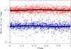 |
Fig. 6 Same as Fig. 5 except for frequency 1.767 c/d. |
| In the text | |
|
Fig. 7 Product of the AOV spectra (after pre-whitening for 1.5561 and 0.034 c/d) of the blue and red passband. Note the occurrence of frequency groups and the relative isolation of the peaks at 1.732 and 1.767 c/d. |
| In the text | |
|
Fig. 8 Time dependence of the frequency (lower panel) and amplitude (upper panel) of the 1.5562-c/d variability in η Cen (red passband: +; blue passband: ×). Frequencies and amplitudes were determined as sliding averages over three-day intervals from sine fits. For comparison, the sine curve fitted to the light curve in Fig. 4 is overplotted with arbitrary scaling and vertical offset (note that the magnitude scale is inverted). |
| In the text | |
|
Fig. 9 The BRITE light curve of μ Cen (in instrumental, mean-subtracted magnitudes; red passband: +; blue passband: ×, vertically offset by 0.15 mag). |
| In the text | |
|
Fig. 10 The Strömgren b light curve of μ Cen as measured by Cuypers et al. (1989). |
| In the text | |
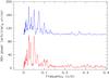 |
Fig. 11 AOV spectra of μ Cen (top: blue channel; bottom: red channel). |
| In the text | |
|
Fig. 12 Blue (top) and red (bottom) AOV spectra of η Cen after pre-whitening for the 1.5562 c/d Štefl frequency; see also Fig. 2. Note the numerous features (“grass”) around 1.55 and 3.1 c/d, but also below both frequency regions. The complex close to 4.8 c/d corresponds to one-third of the satellites’ orbital frequency (fo/ 3). Compare this figure also to Fig. 2. |
| In the text | |
|
Fig. 13 Time-frequency diagram (bottom image: blue passband; top image: red passband) of the Type II frequency group around 1.55 c/d in η Cen, after pre-whitening for the 1.5562 c/d frequency. AOV spectra with a sampling of 0.0005 c/d were calculated over 3 d sliding averages. The frequency interval shown (abscissa) is 1.1–1.7 c/d. For both sub-images the AOV power (white is highest) was separately normalized to the respective mean power to facilitate comparison. The ordinates (in days) have arbitrary zero points. The two data strings have different starting dates but end at about the same time (cf. Fig. 4). |
| In the text | |
Current usage metrics show cumulative count of Article Views (full-text article views including HTML views, PDF and ePub downloads, according to the available data) and Abstracts Views on Vision4Press platform.
Data correspond to usage on the plateform after 2015. The current usage metrics is available 48-96 hours after online publication and is updated daily on week days.
Initial download of the metrics may take a while.