| Issue |
A&A
Volume 588, April 2016
|
|
|---|---|---|
| Article Number | A142 | |
| Number of page(s) | 7 | |
| Section | Atomic, molecular, and nuclear data | |
| DOI | https://doi.org/10.1051/0004-6361/201527826 | |
| Published online | 01 April 2016 | |
Asymmetry in the triplet 3p-4s Mg lines in cool DZ white dwarfs
1 GEPI, Observatoire de Paris, PSL Research University, UMR 8111, CNRS, Université Paris Diderot, Sorbonne Paris Cité, 61 avenue de l’Observatoire, 75014 Paris, France
e-mail: This email address is being protected from spambots. You need JavaScript enabled to view it.
2 Institut d’Astrophysique de Paris, UMR 7095, CNRS, Université Paris VI, 98bis boulevard Arago, 75014 Paris, France
3 Laboratoire de Physique et Chimie Quantique, Université de Toulouse (UPS), UMR 5626, and CNRS, 118 route de Narbonne, 31400 Toulouse, France
4 Département de Physique, Université de Montréal, Montréal, Québec H3C 3J7, Canada
5 Institut de Recherche sur les Exoplanètes (iREx), Université de Montréal, Montréal, Québec H3C 3J7, Canada
Received: 24 November 2015
Accepted: 25 January 2016
Abstract
The purpose of the present work is to make an exhaustive study of the line shape of the triplet 3p-4s Mg line (Mgb triplet), which is perturbed by He in the extreme physical conditions found in the cool atmosphere of DZ white dwarfs. This study is undertaken by inferring both a unified theory of spectral line broadening and ab initio potential energies. Cool white dwarfs require a specific treatment for line broadening owing to the high helium densities that are involved. Beyond the conventional symmetrical Lorentzian core at low density, we show that the line profiles are asymmetrical and have significant additional contributions on the short wavelength side. This blue asymmetry is a consequence of low maxima in the corresponding Mg-He potential energy difference curves at short and intermediate internuclear distances. The new profiles are shown to provide a good fit to an SDSS (Sloan Digital Sky Survey) observation.
Key words: line: profiles / stars: atmospheres / white dwarfs
© ESO, 2016
1. Introduction
Heavy elements are not expected to be found at the surface of old white dwarfs owing to their very high surface gravity. Indeed, metals settle on timescales that are much shorter than the cooling age of these stars, thus leaving behind a pure hydrogen/helium photosphere (Paquette et al. 1986). Yet, traces of heavy elements, such as calcium, magnesium, and iron are commonly detected at the surface of many old white dwarfs (see Koester et al. 2014, and references therein), indicating that an external source must have recently replenished the photosphere. It is now accepted that this source is the accretion from a disk that was formed by the tidal disruption of one or many rocky objects that passed too close to the white dwarf, most likely asteroids or minor planets (Jura & Young 2014; Koester et al. 2014). Hence, these “polluted” white dwarfs can be used as a probe to characterize the chemical composition of rocky material that once orbited main-sequence stars.
To fully exploit the potential of these objects as planetary probes, we need to first obtain accurate photospheric abundances. Indeed, because of the relatively low opacity of the helium atmospheres at lower effective temperatures, photons that escape the star originate from deeper layers where the density is very high. Under these conditions, the emiting atoms can experience multiple simultaneous perturbations with the surrounding helium atoms. A reliable calculation of the line profiles that is applicable in all parts of the line at all densities is the Anderson semi-classical theory (Anderson 1952), which utilizes the Fourier transform (FT) of an autocorrelation function.
The metals most commonly identified at white dwarf’s photospheres are calcium, magnesium, and iron. Calculating their abundances requires accurate description of the line profiles. However, there is a reliance on simplified models of line-broadening physics that remains in most of the code that is in current use. These models, typically use either Lorentzian or quasistatic van der Waals profiles with adjusted empirical parameters.
This paper is a continuation of our studies of sodium and ionized calcium resonance lines that are perturbed by helium (Allard & Alekseev 2014; Allard 2013; Allard et al. 2014). We consider the satellite band that is associated with the transition between the 3p and the 4s levels of a magnesium atom, which is perturbed by dense helium plasma. The purpose of this investigation is to establish the link between the strong asymmetric spectral features that are observed in cool DZ white dwarfs and the existence of a very close blue satellite. The asymmetrical shapes of spectral lines have been extensively investigated for many years because of their importance in experimental and theoretical work (Allard & Kielkopf 1982). The asymmetry in the Mg profile was incorrectly identified as being due to quasistatic broadening by Wehrse & Liebert (1980).
The triplet 3p-4s line profiles of Mg perturbed by helium, are calculated for the physical conditions encountered in the atmospheres of cool white dwarfs. Starting with the Anderson (1952) theory, suitably generalized to include degeneracy, a unified theory of spectral line broadening (Allard et al. 1999) has been developed to calculate neutral atom spectra, given the interaction and the radiative transition moments of relevant states of the radiating atom with other atoms in its environment. Line profile calculations in our work have been done using accurate ab initio potential energies that take into account the long range part (Sect. 2). The theory (Sect. 3) and interpretation (Sect. 4) are similar to that previously reported in (Allard et al. 2009, 2011, 2012; Allard 2012) for interpreting observations of a corona discharge in liquid He. Several theoretical computed profiles are used to illustrate the evolution of the line and satellite with temperatures (Sect. 5). Shift, broadening, and asymmetry are discussed in terms of the evolution of the spectral line shapes with density in Sect. 6. Finally an astrophysical application for a cool DZ white dwarf is reported in Sect. 7.
Molecular to atomic asymptotic energy matching.
2. MgHe diatomic potentials
Significant progress in the description of Mg–He singlet and triplet potential energies has been achieved by Alekseev 20141, but in a small range, R ~ 2.5 to 20 a.u., where R denotes the internuclear distance between the radiator and the perturber. To predict the impact core shift and width, the long range part of the potential energies needs to be accurately determined.
The ab initio calculations of the potentials were made using a large core pseudopotential (Fuentealba et al. 1983) for Mg complemented by operatorial core polarisation potential (CPP), with the MOLPRO package (Werner et al. 2012). For Mg, we built a large basis set that was inspired by the standard (pseudopotential) basis set (Fuentealba et al. 1982) and the one used in rather high Rydberg state calculations (Khemiri et al. 2013) leading to a 10s9p6d3f3g basis set. For He, the huge 30s17p10d6f3g basis set of Deguilhem and coworkers was used (Deguilhem et al. 2009). State-specific orbitals were obtained from CASSCF calculations (Werner & Knowles 1985), where the active space consisted of four electrons distributed in all orbitals up to the 4s of Mg (i.e., a CAS 4,6). These orbitals were then used in subsequent MRCI (Werner & Knowles 1988) calculations to obtain the potential energy curves, as well as static and transition dipole moments for all permitted transitions. The potential curves have been computed using a dense grid of internuclear points ranging from R = 4 to 500 a.u. Potential energy curves V(R) for the MgHe molecule involved in the transition between the 3p and the 4s levels are shown in Fig. 1.
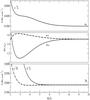 |
Fig. 1 Potential energies for the a, b, and c states of the Mg–He molecule without SO coupling. 4s c3Σ (full line), 3p b3Σ (full line), 3p a3Π (dashed line), and transition dipole moment c-b (full line), c-a (dashed line). |
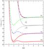 |
Fig. 2 Potential curves correlated with the 3p states without (black) and with inclusion of spin-orbit coupling (red/full: Ω = 0, blue/dash-dot: Ω = 1 and green/dash: Ω = 2) of the Mg–He molecule. The energies are given relative to the potentials without spin-orbit coupling. The fine structure separation is 20.2573 cm-1. |
Spin-orbit interaction is taken into account using the Cohen Schneider scheme where the atomic SO coupling is generalised to the molecule (Cohen & Schneider 1974). It has been shown to work very well for heavy rare gases ionic clusters such as Kr and Xe (Hrivnak et al. 2005). Here, for a ns n′p scheme, two matrices need to be diagonalised, respectively for Ω = 0 and Ω = 1, while for Ω = 2, there is just an energy shift of the
  energy:
![Mathematical equation: \begin{eqnarray*} &&\Omega=0 \\[3mm] && \left(\begin{array}{cccc} E(^{3}P_{\Pi})-\alpha & \alpha & 0 & \alpha\\ \alpha & E(^{3}P_{\Sigma}) & \alpha & 0\\ 0 & \alpha & E(^{3}P_{\Pi})-\alpha & -\alpha\\ \alpha & 0 & -\alpha & E(^{1}P_{\Sigma}) \end{array}\right) \\[3mm] && \Omega=1 \\[3mm] &&\left(\begin{array}{ccc} E(^{3}P_{\Pi}) & \alpha & \alpha\\ \alpha & E(^{3}P_{\Sigma}) & -\alpha\\ \alpha & -\alpha & E(^{1}P_{\Pi}) \end{array}\right) \\[3mm] && \Omega=2 \\[2mm] && E(^{3}P_{\Pi})+\alpha. \end{eqnarray*}](/articles/aa/full_html/2016/04/aa27826-15/aa27826-15-eq32.png) Here, Ω corresponds to the good quantum number in the Hund case c (Ω = Λ + Σ) for the molecule and corresponds to MJ = ML + MS for the atoms.
Here, Ω corresponds to the good quantum number in the Hund case c (Ω = Λ + Σ) for the molecule and corresponds to MJ = ML + MS for the atoms.
For α we have taken 20.2573 cm-1, to recover the correct J = 2−J = 0 atomic splitting. Asymptotically, the  and are degenerated and the matching between the atomic and molecular energies (degeneracies are recalled in paranthesis) is given in Table 1. The degeneracy is lifted by the SO coupling and the states at + α, −α and −2α match the atomic states, J = 2, J = 1, and J = 0, respectively.
For general R, this degeneracy is lifted by molecular interactions. The molecular states are now: a: 1 3Π, b: 1 3Σ, c: 2 3Σ. The He atom remains closed shell, therefore the occupation in Mg mainly controls the identification of the states and the labelling that relates to the Mg atoms still makes sense. The resulting potentials are given in Fig. 2 and compared with the potentials without spin-orbit coupling. Spin-orbit coupling has a huge effect and leads to two very repulsive states correlating to J = 2, two curves with double-well shapes correlating to J = 1 and J = 0, while the two last potentials remain very similar to the 3Π state.
On the other hand, the main difference at short distances between the repulsive walls of the a and b potentials remains after spin-orbit coupling. For the various Ω, all potentials remain at short distances that are either close to the a (the two lowests for Ω = 0, the lowest for Ω = 1 and the Ω = 2) or to the b (the highest for Ω = 0 and Ω = 1) repulsive potentials. We will see the effect on the potential differences in the next section and, consequently, on the line profiles of the different components.
3. Theoretical profiles
Foreign-gas pressure-broadening of spectral lines is due to the difference in the interaction energies of the optical atom (in the initial and final states involved in the radiating or absorbing process) and a foreign colliding atom over a wide range of distances.
As a first approach (Leininger et al. 2015) we used potential energies of the 3p state without SO coupling (Fig. 1). At high He density, the lines 3p  are not resolved, the spin-orbit was not included in our calculations, we were typically in the Hund case b. The line profile depends only on the two individual transitions a 3p3Π → c 4s3Σ and b 3p3Σ → c 4s3Σ.
The prediction of the shape of the 3p → 4s line required us to study ΔV(R), as shown in Fig. 3. The difference potential maxima are respectively 400 and 165 cm-1 for a–c and b–c transitions.
The unified profiles are the Fourier transforms of the autocorrelation functions as given by Eq. (121) of Allard et al. (1999) in which the contributions from the two components of the transition enter with their statistical weights. The unified theory predicts that there will be line satellites centered periodically at frequencies corresponding to integer multiples of the extrema of ΔV.
Figure 4 shows the individual components for comparison, weighted as if they were the only contribution to the profile. The distinct wide shoulder at about 240 cm-1 owing to the 3p3Π → 4s3Σ transition, yields a line satellite in the blue wing that is about 5120 Å (Fig. 3 of Leininger et al. 2015). The other maximum at ΔV= 165 cm-1 does not give the slightest hint of a blue shoulder, the corresponding individual profile simply appears to have a blue asymmetry.
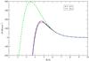 |
Fig. 3 ΔV for the transitions contributing to 3p → 4s line without SO (black lines): 3p3Σ → 4s3Σ and 3p3Π → 4s3Σ. All the other ΔV for the components J = 2 are superimposed (red/full: Ω = 0, blue/dash-dot: Ω = 1 and green/dash: Ω = 2). |
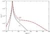 |
Fig. 4 Individual components of the line profile, neglecting the SO coupling, compared to the total profile at T = 6000 K and for nHe = 1020 cm-3. |
To provide opacity data 2 at any He density, we will consider the different components Jn of the triplet using the potentials with inclusion of spin-orbit coupling (Fig. 2). As mentioned before, all potentials remain at short distances either close to the a and b potentials, the values of ΔV for J2 remain almost unchanged (Fig. 3). We did not plot ΔV for J0 and J1 since they are all close to a–c. Figure 5 shows the line shape of the different components Jn of the triplet at nHe = 1020 cm-3 and T = 6000 K. The main change concerns the J2 component. Because of the smaller relative weight of the contribution of the a–c transition, the line satellite is not well-pronounced compared to those appearing in the near wings of J0 and J1 which are strictly due to a–c. Since we are considering a low pressure, the core of the line is described adequately by a Lorentzian, and because of the log scaling in Fig. 5, the Lorentzian is plotted only for J2. In Table 2, we report our computed half-widths at half maximum (HWHM) and shift in the impact approximation for the different components Jn of the triplet at T = 6000 K.
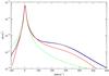 |
Fig. 5 Theoretical absorption cross sections of the components J0 (blue line), J1 (black line), and J2 (red line) compared to the Lorentzian profile for J2 (green/dash line). The density of perturbers is nHe = 1020 cm-3. The temperature is 6000 K. |
Half-width at half maximum (w) and shift (d) (10-20 cm-1/ cm-3) of the components of the triplet lines at T = 6000 K.
4. The influence of close blue satellite on spectral line shape
Several helium-rich white dwarf stars show an asymmetry in the Mgb triplet (many examples can be found in Koester et al. 2011), indicating that the physical conditions present in these stars are such that the impact approximation is no longer valid. Figure 6 shows a typical temperature and pressure structure for one such star, SDSS 1535+1247, the brightest object in the Koester et al. (2011) sample. With densities well above 1020 cm-3 in the line forming region (log τR ~ −3 to 0), the possibility of several atoms interacting strongly is high, and this plays a role in the wavelength of the line center, e.g. the shift of the line, as well as the continuum generated far from the line center. This is indeed what is observed in the spectra of SDSS 1535+1247 (see Fig. 13), where the asymmetric blue wing of the Mg triplet can easily be appreciated.
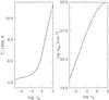 |
Fig. 6 Temperature and He density as a function of Rosseland mean optical depth assuming SDSS 1535+1247 atmospheric parameters (Koester et al. 2011). |
In the next section, we will evaluate collisional profiles of the different components Jn of the triplet for relevant temperatures and densities that are appropriate for modeling helium-rich white dwarf stars. For such high helium density the collisional effects should be treated by using the unified theory presented in Allard et al. (1999) to take into account simultaneous collisions with more than one perturbing atom. The traditional separation of line profiles into a core region to be treated by the impact approximation and a wing region to be treated by the quasistatic approximation fails to be satisfactory when very close line satellites lead to an asymmetrical shape of the line with increasing perturber density. This asymmetry in the Mgb triplet was uncorrectly identified as being due to quasistatic broadening by Wehrse & Liebert (1980) and used in many astrophysical modelings (Kawka et al. 2004; Koester et al. 2011).
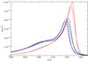 |
Fig. 7 Variation of the line profile with temperature for nHe = 1021 cm-3 for the 3 components J0 (blue line), J1 (black line), and J2 (red line). 4000 K (full line), 6000 K (dashed line), and 8000 K (dashed dotted line). |
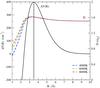 |
Fig. 8 Difference potential energy ΔV(R) in cm-1 (black line) and the temperature dependence of modulated dipole D(R) (color lines) corresponding to the 3p a→ 4s c transition. |
5. Temperature dependence of the line satellite
Collisional line profiles were evaluated for nHe = 1 × 1021 cm-3 from 4000 to 8000 K, the line wings shown in (Fig. 7) are almost unchanged with increasing temperature. While the position of the line satellites critically depends on the interaction potential, their strength depends on both the interaction potentials and the radiative dipole moments, D(Rext), in the internuclear region where the line satellite is formed. In Allard et al. (1999) we defined  as a modulated dipole
 ![Mathematical equation: \begin{equation} D(R) \equiv \tilde{d}_{ee'}[R(t)] = d_{ee'}[R(t)]e^{-\frac{\beta}{2}V_{e}[R(t)] } , \; \label{eq:mod} \end{equation}](/articles/aa/full_html/2016/04/aa27826-15/aa27826-15-eq70.png) (1)where β is the inverse temperature (1 /kT). Here Ve is either the a or b states since we consider absorption profiles due to a–c and b–c transitions. An examination of Fig. 8 shows that the 5080 Å line satellite is formed around Rext = 3.5 Å. The flat dependence in D(R) throughout this region is shown to not alter the amplitude of the satellite (Fig. 7). In this range of temperatures, the strength of the blue wing is not sensitive to the temperature.
(1)where β is the inverse temperature (1 /kT). Here Ve is either the a or b states since we consider absorption profiles due to a–c and b–c transitions. An examination of Fig. 8 shows that the 5080 Å line satellite is formed around Rext = 3.5 Å. The flat dependence in D(R) throughout this region is shown to not alter the amplitude of the satellite (Fig. 7). In this range of temperatures, the strength of the blue wing is not sensitive to the temperature.
6. Density dependence of the collisional profiles
In Figs. 9–11 we show the variation of the absorption cross section at 6000 K with increasing helium density. There is a dramatic change when the density gets larger than 1021 cm-3.
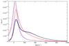 |
Fig. 9 Theoretical absorption cross sections of the components J0 (blue line), J1 (black line), and J2 (red line) compared to the Lorentzian profiles for J0 (blue/dash line) and for J2 (red/dash line). The density of perturbers is nHe = 1021 cm-3. The temperature is 6000 K. |
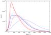 |
Fig. 10 Evolution of the unified profiles of the components J0 (blue lines) and J2 (red lines) with increasing helium density for nHe = 1.75 × 10²¹ (full line), 2 × 10²¹ (dotted line) and to 3 × 1021 cm-3 (dashed line), T = 6000 K. |
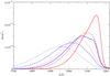 |
Fig. 11 Evolution of the unified profiles of the components J0 (blue lines) and J2 (red lines) with increasing helium density for nHe = 2 × 10²¹ (full line), 3 × 1021 cm-3 (dashed line) and 4 × 1021 cm-3 (dotted line), T = 6000 K. |
6.1. Study of the line parameters
The simplest way of characterizing a line shape is in terms of the parameters, w, the full width at half maximum (FWHM), d, the shift, and the asymmetry (which is computed by taking the ratio of the width at half of the maximum intensity of the blue side to that of the red side). The impact approximation is widely used for describing the central region of pressure-broadened spectral lines at low densities.
We have studied the variations of the line parameters versus the density for T = 6000 K for the J0 and J2 components. To determine these parameters, several theoretical unified profiles have been computed to illustrate the complicated evolution of the triplet line with gas pressure. Figure 12 allows us to understand the complex variation of the line profiles and the line parameters. At low density the core of the theoretical profile is not affected by the blue satellite, hence the width changes linearly with density, the same is true for the shift and, the asymmetry is close to one, like a Lorentzian. We show that striking general features of the shift, width and asymmetry curves occur when the pressure is high enough to blend the satellite and the line core (Figs. 9–11).
6.2. Study of the J0 component
The line satellite becomes higher than the main line for nHe = 2 × 1021 cm-3. Hence, a “discontinuity” appears on the shift; the shift is now being measured from the satellite peak rather than the line peak. An analogous “discontinuity” appears on the asymmetry curve. At this point, the width is measured relative to the half-magnitude of the satellite. The situation is now reversed. The satellite is now regarded as the main line and is broadened by a decreasing “satellite”, when nHe = 4 × 1021 cm-3 the main line has totally disappeared (Fig. 11).
The reason for this transition to very non-linear behavior is that we are first measuring the width proper at lower density. Then, as the density increases and the satellite grows to more than one half the height of the line, we are measuring the combined width of line and satellite.
Moreover, we have known for a long time, since the pioneering work of Cartan & Hindmarsh (1969), that multiple satellites can be observed experimentally at very high densities. A definite observation of multiple perturber satellites was reported in Kielkopf & Allard (1979); they lead to a complicated evolution of the line parameters. In previous papers (Allard 1978; Allard & Biraud 1980; Gilbert et al. 1980; Royer 1980), a theoretical model based upon a simple square-well potential was developed. This model represented the first step to calculations involving more realistic potentials. Even though simple, the model at that stage of development nevertheless provided one with a means of clearly understanding many features in the experimental parameter curves (Ch’en & Garrett 1966; Ch’en et al. 1967, 1969; Garrett & Ch’en 1966; Garrett et al. 1967; Tan & Ch’en 1970).
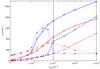 |
Fig. 12 Variation of the width (full line), shift (dashed line) and asymmetry ×100 (dotted line) in the He density range nHe = 5 × 10¹⁹ to 4 × 1021 cm-3 for T = 6000 K. J0 (blue lines) and J2 (red lines). |
6.3. Study of the J2 component
Figures 9–11 reveal that the development of the blue wing leads to the line being overwhelmed by the line satellite, when the density is about 1.75 × 1021 cm-3. When the density reaches 2 × 1021 cm-3, the satellite completely blends with the line seen in Fig. 10. This is a smooth transition for that component compared to the discontinuities observed for J0. As emphasized in Sect. 3, the small relative weight of the 3pa → 4sc transition gives an apparently featureless blue wing. Nevertheless the development of the close satellite leads to the change in the slope of the width and shift for nHe = 2 × 1021cm-3. The asymmetry parameter is then maximum and reaches the value of three.
We see that the profiles and parameters of the triplet 3p-4s of Mg perturbed by helium, are thus very sensitive to helium density. They clearly illustrate how non-linear the non-Lorentzian shapes can become outside the limited range of validity of the impact approximation usually used in stellar and planetary atmosphere modeling.
7. Astrophysical application
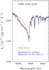 |
Fig. 13 Comparison of the Mg line profiles using the quasistatic profile (blue) and the unified line-shape semi-classical theory (red) for SDSS 1535+1247 (black line). The atmospheric parameters of Koester et al. (2011) are assumed. |
Assuming the atmospheric parameters of Koester et al. (2011) for SDSS 1535+1247, in Fig. 13 we compare the results from using the unified line shape semi-classical theory to that from the quasistatic line profiles (D. Koester, priv. comm.). We note that the magnesium abundance was increased by a factor of 1.8 relative to Koester et al. (2011) to compensate for the fraction of the core absorption that is now shifted into the blue wing. Further minor adjustments to the atmospheric parameters of Koester et al. (2011), which are beyond the scope of this paper, should further improve the accuracy of the fit to the data. We take the relatively good agreement between the observed line shape of the blue wing and our new calculations as a confirmation that the asymmetry of the triplet MgHe line is, indeed, due to the blue satellite band that is associated with the 3p-4s transition.
8. Conclusion
We have performed a theoretical calculation of the triplet MgHe line profiles using a unified theory of spectral line broadening and high quality ab initio potentials. We showed that a line satellite band located in the near blue wing of the Mg lines is responsible of an asymmetry that has not been correctly considered by modelers of cool DZ white dwarfs Wehrse & Liebert (1980), Koester et al. (2011). This effect of this is increasingly important, with He density, and as a result, the line profiles shifting towards the position of the satellite band. The width, shift, and asymmetry of the lines are very dependent on the nature of the interactions between the atoms at short and intermediate distance when the He density gets high. Whereas the potential energies of Alekseev 20141 are computed in a smaller range of internuclear distances, the unified profiles are practically the same as those reported here in the extreme physical conditions of cool DZ white dwarfs.
Previously, Allard et al. (2013) discussed the major importance of close blue satellites that are associated with He-He collisions, the line profiles of the 2p-3s transitions exhibit a similar blue asymmetric behavior. For others alcaline earth metals, similar effects can be expected since comparable electronic distributions and interactions with He could be expected. Therefore asymmetric shapes due to close blue satellites can also be expected for them, in particular for Ca broadened by collisions with He, the heavier neighboring alcaline earth metal.
Complete tables are available on request from NFA.
Acknowledgments
The authors thank the referee, Paul Barklem, for helpful comments and suggestions that have improved the clarity of the paper. One of us (NFA) would like to acknowledge V. Alekseev for kindly providing the Mg–He molecular potentials and dipole moments before publication.
References
- Allard, N. F. 1978, J. Phys. B: At. Mol. Opt. Phys., 11, 1383 [Google Scholar]
- Allard, N. F. 2012, J. Phys. Conf. Ser., 397, 012065 [NASA ADS] [CrossRef] [Google Scholar]
- Allard, N. F. 2013, in EAS Pub. Ser., 63, 403 [Google Scholar]
- Allard, N. F., & Alekseev, V. A. 2014, Adv. Space Res., 54, 1248 [NASA ADS] [CrossRef] [Google Scholar]
- Allard, N. F., & Biraud, Y. G. 1980, J. Quant. Spectr. Rad. Trans., 23, 253 [NASA ADS] [CrossRef] [Google Scholar]
- Allard, N. F., & Kielkopf, J. F. 1982, Rev. Mod. Phys., 54, 1103 [NASA ADS] [CrossRef] [Google Scholar]
- Allard, N. F., Royer, A., Kielkopf, J. F., & Feautrier, N. 1999, Phys. Rev. A, 60, 1021 [NASA ADS] [CrossRef] [Google Scholar]
- Allard, N. F., Deguilhem, B., Gadéa, F. X., Bonifaci, N., & Denat, A. 2009, Europhys. Lett., 88, 53002 [NASA ADS] [CrossRef] [EDP Sciences] [Google Scholar]
- Allard, N. F., Bonifaci, N., & Denat, A. 2011, EpJ D, 61, 365 [NASA ADS] [CrossRef] [EDP Sciences] [Google Scholar]
- Allard, N. F., Monari, A., Deguilhem, B., & Gadéa, F. X. 2012, J. Phys. Conf. Ser., 397, 012035 [NASA ADS] [CrossRef] [Google Scholar]
- Allard, N. F., Deguilhem, B., Monari, A., Gadéa, F. X., & Kielkopf, J. F. 2013, A&A, 559, A70 [NASA ADS] [CrossRef] [EDP Sciences] [Google Scholar]
- Allard, N. F., Homeier, D., Guillon, G., Viel, A., & Kielkopf, J. 2014, J. Phys. Conf. Ser., 548, 012006 [NASA ADS] [CrossRef] [Google Scholar]
- Anderson, P. W. 1952, Phys. Rev., 86, 809 [NASA ADS] [CrossRef] [Google Scholar]
- Cartan, D. G. M., & Hindmarsh, W. R. 1969, J. Phys. B: At. Mol. Opt. Phys., 2, 1396 [NASA ADS] [CrossRef] [Google Scholar]
- Ch’en, S. Y., & Garrett, R. O. 1966, Phys. Rev., 144, 59 [NASA ADS] [CrossRef] [Google Scholar]
- Ch’en, S. Y., Looi, E. C., & Garrett, R. O. 1967, Phys. Rev., 155, 38 [NASA ADS] [CrossRef] [Google Scholar]
- Ch’en, S. Y., Gilbert, D. E., & Tan, D. K. L. 1969, Phys. Rev., 184, 51 [NASA ADS] [CrossRef] [MathSciNet] [Google Scholar]
- Cohen, J. S., & Schneider, B. 1974, J. Chem. Phys., 61, 3230 [NASA ADS] [CrossRef] [Google Scholar]
- Deguilhem, B., Leininger, T., Gadea, F. X., & Dickinson, A. S. 2009, J. Phys. B: At. Mol. Opt. Phys., 42, 015102 [NASA ADS] [CrossRef] [Google Scholar]
- Fuentealba, P., Preuss, H., Stoll, H., & Szentplay, L. 1982, Chem. Phys. Lett., 89, 418 [NASA ADS] [CrossRef] [Google Scholar]
- Fuentealba, P., Stoll, H., Szentpaly, L., Schwerdtfeger, P., & Preuss, H. 1983, J. Phys. B, 16, L323 [NASA ADS] [CrossRef] [Google Scholar]
- Garrett, R. O., & Ch’en, S. Y. 1966, Phys. Rev., 144, 1 [CrossRef] [Google Scholar]
- Garrett, R. O., Ch’en, S. Y., & Looi, E. C. 1967, Phys. Rev., 156, 1 [CrossRef] [Google Scholar]
- Gilbert, D. E., Allard, N. F., & Ch’en, S. Y. 1980, J. Quant. Spectr. Rad. Trans., 23, 201 [Google Scholar]
- Hrivnak, D., Kalus, R., & Gadéa, F. X. 2005, Europhys. Lett., 71, 42 [NASA ADS] [CrossRef] [EDP Sciences] [Google Scholar]
- Jura, M., & Young, E. D. 2014, Rev. Earth Planet. Sci., 42, 45 [CrossRef] [Google Scholar]
- Kawka, A., Vennes, S., & Thorstensen, J. R. 2004, AJ, 127, 1702 [NASA ADS] [CrossRef] [Google Scholar]
- Khemiri, N., Dardouri, R., Oujia, B., & Gadéa, F. X. 2013, J. Phys. Chem., 117, 8915 [CrossRef] [Google Scholar]
- Kielkopf, J. F., & Allard, N. F. 1979, Phys. Rev. Lett., 43, 196 [NASA ADS] [CrossRef] [Google Scholar]
- Koester, D., Girven, J., Gänsicke, B. T., & Dufour, P. 2011, A&A, 530, A114 [NASA ADS] [CrossRef] [EDP Sciences] [Google Scholar]
- Koester, D., Gänsicke, B. T., & Farihi, J. 2014, A&A, 566, A34 [NASA ADS] [CrossRef] [EDP Sciences] [Google Scholar]
- Leininger, T., Gadéa, F. X., & Allard, N. F. 2015, in SF2A-2015: Proc. Annual meeting of the French Society of Astronomy and Astrophysics, eds. F. Martins, S. Boissier, V. Buat, L. Cambrésy, & P. Petit, 397 [Google Scholar]
- Paquette, C., Pelletier, C., Fontaine, G., & Michaud, G. 1986, ApJS, 61, 197 [NASA ADS] [CrossRef] [Google Scholar]
- Royer, A. 1980, Phys. Rev. A, 22, 1625 [NASA ADS] [CrossRef] [Google Scholar]
- Tan, D. K., & Ch’en, S. Y. 1970, Phys. Rev., 2, 1 [CrossRef] [Google Scholar]
- Wehrse, R., & Liebert, J. 1980, A&A, 86, 139 [NASA ADS] [Google Scholar]
- Werner, H. J., & Knowles, P. J. 1985, J. Chem. Phys., 82, 5053 [NASA ADS] [CrossRef] [Google Scholar]
- Werner, H. J., & Knowles, P. J. 1988, J. Chem. Phys., 89, 5803 [NASA ADS] [CrossRef] [Google Scholar]
- Werner, H.-J., Knowles, P. J., Knizia, G., et al. 2012, MOLPRO, version 2012.1, a package of ab initio programs [Google Scholar]
All Tables
Half-width at half maximum (w) and shift (d) (10-20 cm-1/ cm-3) of the components of the triplet lines at T = 6000 K.
All Figures
|
Fig. 1 Potential energies for the a, b, and c states of the Mg–He molecule without SO coupling. 4s c3Σ (full line), 3p b3Σ (full line), 3p a3Π (dashed line), and transition dipole moment c-b (full line), c-a (dashed line). |
| In the text | |
|
Fig. 2 Potential curves correlated with the 3p states without (black) and with inclusion of spin-orbit coupling (red/full: Ω = 0, blue/dash-dot: Ω = 1 and green/dash: Ω = 2) of the Mg–He molecule. The energies are given relative to the potentials without spin-orbit coupling. The fine structure separation is 20.2573 cm-1. |
| In the text | |
|
Fig. 3 ΔV for the transitions contributing to 3p → 4s line without SO (black lines): 3p3Σ → 4s3Σ and 3p3Π → 4s3Σ. All the other ΔV for the components J = 2 are superimposed (red/full: Ω = 0, blue/dash-dot: Ω = 1 and green/dash: Ω = 2). |
| In the text | |
|
Fig. 4 Individual components of the line profile, neglecting the SO coupling, compared to the total profile at T = 6000 K and for nHe = 1020 cm-3. |
| In the text | |
|
Fig. 5 Theoretical absorption cross sections of the components J0 (blue line), J1 (black line), and J2 (red line) compared to the Lorentzian profile for J2 (green/dash line). The density of perturbers is nHe = 1020 cm-3. The temperature is 6000 K. |
| In the text | |
|
Fig. 6 Temperature and He density as a function of Rosseland mean optical depth assuming SDSS 1535+1247 atmospheric parameters (Koester et al. 2011). |
| In the text | |
|
Fig. 7 Variation of the line profile with temperature for nHe = 1021 cm-3 for the 3 components J0 (blue line), J1 (black line), and J2 (red line). 4000 K (full line), 6000 K (dashed line), and 8000 K (dashed dotted line). |
| In the text | |
|
Fig. 8 Difference potential energy ΔV(R) in cm-1 (black line) and the temperature dependence of modulated dipole D(R) (color lines) corresponding to the 3p a→ 4s c transition. |
| In the text | |
|
Fig. 9 Theoretical absorption cross sections of the components J0 (blue line), J1 (black line), and J2 (red line) compared to the Lorentzian profiles for J0 (blue/dash line) and for J2 (red/dash line). The density of perturbers is nHe = 1021 cm-3. The temperature is 6000 K. |
| In the text | |
|
Fig. 10 Evolution of the unified profiles of the components J0 (blue lines) and J2 (red lines) with increasing helium density for nHe = 1.75 × 10²¹ (full line), 2 × 10²¹ (dotted line) and to 3 × 1021 cm-3 (dashed line), T = 6000 K. |
| In the text | |
|
Fig. 11 Evolution of the unified profiles of the components J0 (blue lines) and J2 (red lines) with increasing helium density for nHe = 2 × 10²¹ (full line), 3 × 1021 cm-3 (dashed line) and 4 × 1021 cm-3 (dotted line), T = 6000 K. |
| In the text | |
|
Fig. 12 Variation of the width (full line), shift (dashed line) and asymmetry ×100 (dotted line) in the He density range nHe = 5 × 10¹⁹ to 4 × 1021 cm-3 for T = 6000 K. J0 (blue lines) and J2 (red lines). |
| In the text | |
|
Fig. 13 Comparison of the Mg line profiles using the quasistatic profile (blue) and the unified line-shape semi-classical theory (red) for SDSS 1535+1247 (black line). The atmospheric parameters of Koester et al. (2011) are assumed. |
| In the text | |
Current usage metrics show cumulative count of Article Views (full-text article views including HTML views, PDF and ePub downloads, according to the available data) and Abstracts Views on Vision4Press platform.
Data correspond to usage on the plateform after 2015. The current usage metrics is available 48-96 hours after online publication and is updated daily on week days.
Initial download of the metrics may take a while.