| Issue |
A&A
Volume 588, April 2016
|
|
|---|---|---|
| Article Number | A150 | |
| Number of page(s) | 13 | |
| Section | Astrophysical processes | |
| DOI | https://doi.org/10.1051/0004-6361/201527731 | |
| Published online | 04 April 2016 | |
Magnetic flux concentrations from turbulent stratified convection⋆
1 ReSoLVE Centre of Excellence, Department of Computer Science, Aalto University, PO Box 15400, 00076 Aalto, Finland
e-mail: This email address is being protected from spambots. You need JavaScript enabled to view it.
2 Department of Physics, Gustaf Hällströmin katu 2a (PO Box 64), University of Helsinki, 00014 Helsinki, Finland
3 NORDITA, KTH Royal Institute of Technology and Stockholm University, Roslagstullsbacken 23, 10691 Stockholm, Sweden
4 Department of Astronomy, AlbaNova University Center, Stockholm University, 10691 Stockholm, Sweden
5 JILA and Department of Astrophysical and Planetary Sciences, Box 440, University of Colorado, Boulder, CO 80303, USA
6 Laboratory for Atmospheric and Space Physics, 3665 Discovery Drive, Boulder, CO 80303, USA
7 Department of Mechanical Engineering, Ben-Gurion University of the Negev, PO Box 653, 84105 Beer-Sheva, Israel
Received: 12 November 2015
Accepted: 20 December 2015
Abstract
Context. The formation of magnetic flux concentrations within the solar convection zone leading to sunspot formation is unexplained.
Aims. We study the self-organization of initially uniform sub-equipartition magnetic fields by highly stratified turbulent convection.
Methods. We perform simulations of magnetoconvection in Cartesian domains representing the uppermost 8.5−24 Mm of the solar convection zone with the horizontal size of the domain varying between 34 and 96 Mm. The density contrast in the 24 Mm deep models is more than 3 × 10³ or eight density scale heights, corresponding to a little over 12 pressure scale heights. We impose either a vertical or a horizontal uniform magnetic field in a convection-driven turbulent flow in set-ups where no small-scale dynamos are present. In the most highly stratified cases we employ the reduced sound speed method to relax the time step constraint arising from the high sound speed in the deep layers. We model radiation via the diffusion approximation and neglect detailed radiative transfer in order to concentrate on purely magnetohydrodynamic effects.
Results. We find that super-equipartition magnetic flux concentrations are formed near the surface in cases with moderate and high density stratification, corresponding to domain depths of 12.5 and 24 Mm. The size of the concentrations increases as the box size increases and the largest structures (20 Mm horizontally near the surface) are obtained in the models that are 24 Mm deep. The field strength in the concentrations is in the range of 3–5 kG, almost independent of the magnitude of the imposed field. The amplitude of the concentrations grows approximately linearly in time. The effective magnetic pressure measured in the simulations is positive near the surface and negative in the bulk of the convection zone. Its derivative with respect to the mean magnetic field, however, is positive in most of the domain, which is unfavourable for the operation of the negative effective magnetic pressure instability (NEMPI). Simulations in which a passive vector field is evolved do not show a noticeable difference from magnetohydrodynamic runs in terms of the growth of the structures. Furthermore, we find that magnetic flux is concentrated in regions of converging flow corresponding to large-scale supergranulation convection pattern.
Conclusions. The linear growth of large-scale flux concentrations implies that their dominant formation process is a tangling of the large-scale field rather than an instability. One plausible mechanism that can explain both the linear growth and the concentration of the flux in the regions of converging flow pattern is flux expulsion. A possible reason for the absence of NEMPI is that the derivative of the effective magnetic pressure with respect to the mean magnetic field has an unfavourable sign. Furthermore, there may not be sufficient scale separation, which is required for NEMPI to work.
Key words: convection / turbulence / sunspots
Movies associated to Figs. 4 and 5 are available in electronic form at http://www.aanda.org
© ESO, 2016
1. Introduction
The current paradigm of sunspot formation relies on the existence of strong magnetic flux tubes (of the order of 105 G) created by some unknown mechanism at the base of the convection zone or just below it. Their buoyant rise to the solar surface is thought to lead to sunspot formation (Parker 1955). This idea has also profoundly influenced solar dynamo modelling: in the so-called flux transport models a highly non-local α-effect is used to parametrize the rise of toroidal flux tubes from the tachocline to form poloidal fields near the surface. A single-cell meridional flow is then supposed to carry the surface poloidal field back to the tachocline where it is sheared back to toroidal form and amplified to close the dynamo loop (e.g. Choudhuri et al. 1995, 2007; Dikpati & Charbonneau 1999; Dikpati & Gilman 2006).
Although superficially plausible, these concepts face several theoretical difficulties: the generation and storage of sufficiently strong magnetic fields has proven to be difficult (e.g. Ghizaru et al. 2010; Guerrero & Käpylä 2011), the stability of the tachocline has been questioned in the case of such strong fields (Arlt et al. 2005), and there are helioseismic indications (Schad et al. 2013; Zhao et al. 2013) and numerical evidence (e.g. Käpylä et al. 2014; Passos et al. 2015; Featherstone & Miesch 2015) that the meridional circulation pattern of the Sun is likely to consist of multiple cells. Lastly, the rotational speeds of active regions are also consistent with the idea that spots are formed near the surface (Brandenburg 2005), which calls for a new mechanism of sunspot formation.
One possibility is the negative effective magnetic pressure instability (NEMPI) in highly stratified turbulence, which results from the reduction of the total (hydrodynamic plus magnetic) turbulent pressure caused by large-scale magnetic fields. As a result, the effective magnetic pressure (the sum of non-turbulent and turbulent contributions to the large-scale magnetic pressure) becomes negative and a large-scale magnetohydrodynamic instability can become excited. This instability does not produce new magnetic flux, but redistributes the large-scale magnetic field so that the regions with super-equipartition magnetic fields are separated by regions with weak magnetic field. This effect has been thoroughly studied analytically (e.g. Kleeorin et al. 1989, 1990, 1993, 1996; Kleeorin & Rogachevskii 1994; Rogachevskii & Kleeorin 2007) and more recently numerically (e.g. Brandenburg et al. 2010, 2012; Kemel et al. 2012b; Käpylä et al. 2012a, and references therein). Further numerical studies have confirmed the existence of NEMPI in direct numerical simulations (DNS) of forced turbulence with weak imposed horizontal (Brandenburg et al. 2011) and vertical (Brandenburg et al. 2013) magnetic fields, and in a two-layer system with an upper unforced coronal layer and a lower forced layer (Warnecke et al. 2013, 2016). With NEMPI, even uniform, sub-equipartition magnetic fields can lead to flux concentrations if there is sufficient scale separation between the forcing scale and the size of the domain in highly stratified turbulence. This mechanism is compatible with a shallow origin of sunspots. Furthermore, numerical simulations of convective dynamos produce diffuse magnetic fields throughout the convection zone (e.g. Ghizaru et al. 2010; Käpylä et al. 2012b; Yadav et al. 2015; Augustson et al. 2015), which could act as the seed field for NEMPI.
An entirely different kinematic process that can form magnetic concentrations is flux expulsion where magnetic fields are expelled from regions of rapid motion. A classical example is a convection cell where fields are swept away from the diverging upflows of granules into intergranular lanes and vertices to form concentrations (Clark 1965; Weiss 1966). Results from relatively weakly stratified numerical simulations of convection can be explained by this process (e.g. Tao et al. 1998; Kitiashvili et al. 2010; Tian & Petrovay 2013), but its role in the presence of strong stratification has not yet been studied. A further possibility is a mean-field instability caused by the suppression of turbulent heat flux by magnetic fields. Such a suppression causes a concentration of the magnetic field, which causes enhanced quenching of convection and further concentration of the field (Kitchatinov & Mazur 2000).
Realistic numerical simulations of solar surface convection in Cartesian domains including radiation transport and ionization are now routinely used to study the structure of sunspots and active regions (e.g. Rempel et al. 2009a,b; Cheung et al. 2010). These models, however, do not address the question of sunspot formation, as the field configuration is controlled by prescribed boundary conditions at the base of the layer. A more self-consistent approach is adopted in the model of Stein & Nordlund (2012) where a 1 kG purely horizontal field is advected through the bottom boundary of the highly stratified gas in their domain, mimicking the emergence of flux from deeper layers. In this set-up, encompassing the top 20 Mm of the solar convection zone, the magnetic field ultimately forms a structure which is buoyantly unstable and rises to the surface to form a small bipolar spot pair. The authors relate the formation of the structure with the large-scale supergranular convection in the deep layers of their simulation, which would be qualitatively consistent with flux expulsion. However, this conclusion is based on a single experiment and these results have yet to be put into a theoretical framework that would allow these results to be generalized to other conditions.
Based on the recent success in the detection of NEMPI in forced turbulence set-ups, it is of great interest to study whether it can also be excited in convection, especially in circumstances similar to those in the study of Stein & Nordlund (2012). Earlier work on the subject revealed the existence of a negative effective magnetic pressure caused by a negative contribution of turbulent convection, but NEMPI was not observed (Käpylä et al. 2012a, 2013). The failure to excite NEMPI in the earlier models is possibly related to insufficient density stratification and poor separation of scales. We set out to study magnetic structure formation with improved high-resolution local convection simulations that are constructed so that they should be more favourable for NEMPI to be excited. However, we also consider other processes, namely flux expulsion, that can explain magnetic structure formation in our simulations.
2. The model
As a basis for our model we use the set-up from Käpylä et al. (2013) with several improvements in order to increase the density stratification and scale separation. First, we use a thin cooling layer at the top where the temperature is cooled toward a constant value. As a consequence, the density decreases exponentially in this region. Second, instead of regular constant kinematic viscosity, we apply a version of Smagorinsky viscosity (Haugen & Brandenburg 2006) in the highest resolution cases to increase the effective fluid Reynolds number and degree of scale separation. Third, to facilitate computations with the increased stratification, which leads to low Mach numbers at the base of the convectively unstable layer, we apply the so-called reduced sound speed method (Rempel 2005; Hotta et al. 2012, 2014) to alleviate the time step constraint.
We solve the compressible hydromagnetics equations, ![Mathematical equation: \begin{eqnarray} &&\frac{\pd \bm A}{\pd t} = {\bm u}\times{\bm B} - \eta \mu_0 {\bm J}, \\ &&\frac{\pd \rho}{\pd t} = -\frac{1}{\xi^2} \bm\nabla\cdot(\rho \bm{u}), \\ &&\frac{D\bm{u}}{Dt} = \bm{g} + \frac{1}{\rho} \left[\bm\nabla \cdot(2\nu\rho\bm{\mathsf{S}})-\bm\nabla p + {\bm J} \times {\bm B}\right], \\ &&T\frac{D s}{Dt} = \frac{1}{\rho}\left[\bm\nabla \cdot (K \bm\nabla T + \chiSGS \rho T \bm\nabla s) + \mu_0\eta {\bm J}^2\right] + 2\nu \bm{\mathsf{S}}^2 + \Gamma , \label{equ:ss} \end{eqnarray}](/articles/aa/full_html/2016/04/aa27731-15/aa27731-15-eq9.png) where A is the magnetic vector potential, u is the velocity, B = B0 + ∇ × A is the magnetic field, B0 is the imposed magnetic field,
where A is the magnetic vector potential, u is the velocity, B = B0 + ∇ × A is the magnetic field, B0 is the imposed magnetic field,  is the current density, η is the magnetic diffusivity, μ0 is the vacuum permeability, ρ is the density, ξ is the sound speed reduction factor, D/Dt = ∂/∂t + u·∇ is the advective time derivative,
  is the gravitational acceleration, ν is the kinematic viscosity, K is the radiative heat conductivity, χSGS is the subgrid scale (SGS) heat conductivity, Γ describes the cooling applied at the surface, s is the specific entropy, T is the temperature, and p is the pressure. The fluid obeys the ideal gas law with p = (γ−1)ρe, where γ = cP/cV = 5/3 is the ratio of specific heats, cP and cV, at constant pressure and constant volume, respectively, and e = cVT is the internal energy. The traceless rate-of-strain tensor S is given by
  (5)For the viscosity we either apply constant kinematic viscosity ν = ν0 or the Smagorinsky viscosity
  , where Δ is the filtering scale (here the grid spacing) and Ck = 0.35 has been found suitable.
For the sound speed reduction factor ξ we either use a constant value of unity when there is no reduction or a profile that matches the vertical stratification of sound speed. The latter choice leads to an effective sound speed which is constant in the whole domain. In the latter case the gain in the time step is roughly a factor of five in comparison to the ξ = 1 case in the runs with the greatest vertical extent.
The depth of the layer is Lz = d and the horizontal extents in the x and y directions are Lh = 4 d. We consider three values of Lz that correspond to 8.5, 12.5, and 24 Mm in physical units; see Sect. 2.3. The top and bottom boundaries are impenetrable and stress free for the flow  (6)and the magnetic field (not including the imposed field) is assumed to be either perfectly vertical or horizontal:
  The energy flux at the lower boundary is fixed
  (9)At the top boundary the temperature is fixed. The radiative conductivity is given by K = ρcPχ, where χ is assumed constant throughout the domain. For χSGS we use a profile so that it has a constant value
  in the lower 20 per cent of the domain and connects smoothly to a value
  in the middle part. In the layer consisting of the uppermost four per cent of the box χSGS drops smoothly to zero.
To maximize the density contrast within the convection zone, we omit a stably stratified layer below it. We add a nearly isothermal cooling layer at the top where the density stratification is also strong. The cooling term Γ relaxes the temperature toward the value at the surface  (10)where f(z) = 1 in the cooling layer above z = zcool and zero elsewhere, and L0 is a cooling luminosity. The pressure scale height in the cooling layer is given by
  (11)In this set-up convection transports most of the flux, whereas radiative diffusion is only important near the bottom of the domain. We start hydrodynamic progenitor runs from isentropic stratifications throughout and apply the cooling above zcool. In the thermally relaxed states we obtain density contrasts, Γρ = ρbot/ρtop, of 230 (Set A), 900 (Set B), and 3.2 × 10³ (Set C) in the three sets of runs; see Table 1. The corresponding density contrasts within the convectively unstable region are denoted
  , and are in the range 60–320 for Sets A–C. The horizontally averaged profiles of density and pressure, along with the corresponding scale heights and the specific entropy, are shown in Fig. 1.
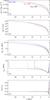 |
Fig. 1 Comparison of the stratifications of our three hydrodynamic runs A00 (black), B00 (red), and C00 (blue) showing density a), pressure b), the density (solid lines) and pressure scale heights (dashed lines) c), correlation length lcorr = 2π/kωd), and specific entropy e). |
2.1. Diagnostics
We define the fluid and magnetic Reynolds numbers as  (12)where urms is the root-mean-square value of the volume averaged velocity and k1 = 2π/d. We also define Prandtl numbers as
  (13)and the Rayleigh number
  (14)where zm = 0.5 d denotes the middle of the unstable layer. In many of the simulations considered here, only the magnetic Reynolds number is well defined because we are using the Smagorinsky scheme for the viscosity. The normalized energy flux is given by
  (15)where the input flux F0, density ρ, and the sound speed
  are evaluated at the lower boundary. We also define the Taylor microscale wavenumber
  (16)which is used in the estimate of the correlation length lcorr = 2π/kω plotted in Fig. 1d. Here ω = ∇ × u. In isotropically forced turbulence, kω is proportional to the square root of the Reynolds number based on the integral wavenumber; see Fig. 3 in Candelaresi & Brandenburg (2013). Calculating the integral wavenumber is usually done via energy spectra, but in stratified convection these spectra change significantly with height, making this approach less practical. The equipartition field strength is defined as
  (17)In the following, averaging over the xy plane is also indicated by an overbar. We typically apply concurrent horizontal and temporal averages to present our results. However, in the cases with an imposed horizontal field we sometimes average along the imposed field, which is mentioned explicitly when applied. In order to extract the large-scale flows generated in the simulations we perform temporal averaging over snapshots without spatial averaging in Sect. 3.3. We use grid resolutions of up to 10243. The computations were performed with the Pencil Code1.
Summary of the sets of runs.
2.2. Modelling strategy
Making the simulation domain deeper and thus increasing the density stratification in convection simulations implies that the sound speed in the deep layers becomes very large and limits the time step. We use the above-mentioned reduced sound speed method to overcome this problem. Furthermore, the pressure scale height near the surface becomes small, necessitating high spatial resolution. We also choose a sufficiently low input flux such that the Mach number near the surface remains sufficiently below unity. This implies a small radiative diffusivity χ = K/ρcP and a long thermal relaxation time, which would require prohibitive computational resources if the simulations were run from scratch.
To address these difficulties, we first evolve hydrodynamic runs where the horizontal extent is reduced by a factor of between four and eight to save computational time. Once these runs have relaxed sufficiently, we replicate them onto a larger horizontal domain and introduce a localized small-scale perturbation in one of the subdomains to break the symmetry introduced in the replication. The system loses the symmetry within a few convective turnovers. We continue to run these hydrodynamical progenitor runs for several tens of convective turnover times before introducing a uniform magnetic field into the system.
2.3. Application to solar parameters
In order to make a comparison with the Sun, it is convenient to transform the results into physical units. This can be done in several ways, which can place the computational domain at different depths in the solar convection zone. As the sunspots are manifestations of the solar magnetic field at the surface, it is logical to place the computational domain near the surface. We assume that the pressure scale height, gas density, and temperature at the surface are the same as in the Sun, i.e.  m, ρ⊙ = 2.5 × 10⁻⁴ kg m-3, and T⊙ = 5800 K defining the units of length, density, and temperature, respectively. Furthermore, we take the acceleration due to gravity to have the solar surface value g⊙ = 274 m s-2, and we use the permeability of vacuum μ0 = 4π × 10-7 N A-2 to derive the unit of magnetic field. With these choices we obtain
 ![Mathematical equation: \begin{eqnarray} &&\left[x\right] = \Hp^{(\rm cool)} = \Hp^{(\odot)},\\ &&\left[t\right] = (\Hp^{(\rm cool)}/g)^{1/2} = (\Hp^{(\odot)}/g_\odot)^{1/2},\\ &&\left[\rho\right] = \rho_{\rm top} = \rho_\odot,\\ &&\left[T\right] = T_{\rm cool} = T_\odot,\\ &&\left[B\right] = \left(\mu_0 \rho_{\rm top} g \Hp^{(\rm cool)}\right)^{1/2} = \left(\mu_0 \rho_\odot g_\odot \Hp^{(\odot)}\right)^{1/2}, \end{eqnarray}](/articles/aa/full_html/2016/04/aa27731-15/aa27731-15-eq102.png) where ρtop = ρ(z = 0) is the surface density, while
where ρtop = ρ(z = 0) is the surface density, while  and Tcool are the pressure scale height and temperature at the top of the cooling layer, respectively.
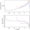 |
Fig. 2 Profiles of horizontally averaged rms velocity urms (top, a)) and equipartition magnetic field Beq (bottom, b)) from the same runs as in Fig. 1 in units of m s-1 and kG, respectively. |
The profiles of horizontally averaged rms velocity and the equipartition magnetic field strength Beq = ⟨ μ0ρu2 ⟩ 1/2 from the hydrodynamic progenitor runs for each of our density stratifications are shown in Fig. 2. The depths of the domains are now 8.5 Mm in Set A, 12.5 Mm in Set B, and 24 Mm in Set C with horizontal sizes of 34, 50, and 96 Mm, respectively. The box in our Set C is comparable to the domain size used by Stein & Nordlund (2012). We find that the velocities near the surface are of the order of 2−3 km s-1, which is similar to the convective velocities observed in the Sun and also obtained from mixing length theory (e.g. Stix 2002). The lower overall velocity in Run C00 is due to a lower input energy flux than in the other runs, which is due to the lower value of K adopted in order to limit the Mach number near the surface. Using the mixing length model of Stix (2002), we note that we obtain a value of ℱ ≈ 2.7 × 10⁻⁷ in the Sun at a depth of roughly 24 Mm. The equipartition magnetic field strength is of the order of 3 kG in Sets B and C. The lower value in Set A is due to the overall lower density in the interior for the runs in that set.
Using these values, the imposed magnetic field strength in Set C, where the clearest indications of flux concentrations are visible, is in the range 230–920 G; see Table 2. The maximum strength of the concentrations shown (Figs. 4 and 5) is in the range 3–5 kG and the size of the largest field concentrations in our simulations are of the order of 20 Mm. Both of these values are in the range observed for sunspots.
Summary of the runs.
3. Results
We perform three sets of simulations in which we increase the size of the domain systematically while keeping the box aspect ratio fixed; see Table 1. We study the cases of horizontal and vertical imposed fields and analyse the detected flux concentrations separately for the two cases. We also measure the effective magnetic pressure from all runs and study whether NEMPI can be the explanation for the observed features.
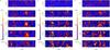 |
Fig. 3 a) Mean magnetic field component |
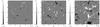 |
Fig. 4 Vertical magnetic field Bz near the surface at a depth of 0.6 Mm from representative snapshots of Runs C2h (left panel), C3h (middle), and C4h (right). The magnetic field scale is clipped at ± 3 kG in each panel. The maximum field strengths obtained are of the order of 5 kG. Animation associated with Run C4h can be found online and at http://research.ics.aalto.fi/cmdaa/group-Movies.shtml. |
3.1. Imposed horizontal field
Early studies of negative effective magnetic pressure and NEMPI in turbulent convection have been performed with an imposed horizontal field (Käpylä et al. 2012a, 2013). This choice is motivated by the anticipated presence of a diffuse, azimuthally dominated large-scale field in the bulk of the solar convection zone. The origin of such a field could be, e.g., an αΩ-type dynamo (Warnecke et al. 2014). When NEMPI was excited, magnetic field concentrations were best detected in averages taken along the direction of the imposed field (Brandenburg et al. 2011; Kemel et al. 2012a, 2013) if the scale separation between forcing scale and the size of the box is smaller than 30. We show two such cases for Runs A3h and C1h with the lowest and highest stratifications in Figs. 3a and b, respectively. We find flux concentrations with maximum field strength of the order of 1 kG, which is roughly four times the imposed field strength. This is similar to what was obtained in the above-mentioned studies employing forced turbulence clearly showing NEMPI.
In the present case, the flux concentrations are associated with large-scale downflows (black/white arrows in Fig. 3). The concentrations become visible near the surface in regions of converging flows. In the 8.5 Mm domain the structures descend to a depth of roughly 6 Mm in five hours; see Fig. 3a. The timescale in Run C1h appears similar (second panel from the top of Fig. 3b) and the concentration reaches the bottom of the domain in roughly 25 h, corresponding to roughly ten large-scale convective turnover times. This is similar to the so-called potato sack effect where horizontal magnetic structures become heavier than their surroundings, often observed as a consequence of the negative effective magnetic pressure. This effect was found in both DNS and mean-field simulations (MFS) of forced turbulence (Brandenburg et al. 2011; Kemel et al. 2013), where the downflows of the magnetic concentrations can be directly associated with the negative effective magnetic pressure. In turbulent convection, the potato sack effect was previously found only in MFS (Käpylä et al. 2012a). In the present study we detect a similar effect for the first time in DNS and LES of convection; see Figs. 3a and b. On the other hand, in convection, downflows occur naturally without the presence of the negative effective magnetic pressure, so it is not clear a priori whether these downflows are affected or even driven by the magnetic field, as was found in isothermal forced turbulence, where no thermal buoyancy is possible.
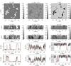 |
Fig. 5 Top row: vertical magnetic field Bz, vertical velocity uz, and temperature T, respectively, at z = 0.6 Mm for Run C1v. The second and third rows show vertical cuts from cuts through y = 15.9 Mm and y = −5.8 Mm. In the rightmost panels we show the |

As a control, we run one of the models (Run A3h) from the same initially hydrodynamic snapshot and neglect the Lorentz-force and Ohmic heating. In this simulation the induction equation does not affect the flow and the magnetic field is a passive vector. We show in Fig. 3c the passive vector evolution corresponding to the magnetic field evolution in Fig. 3a. We find that a flux concentration forms near x ≈ 14.5 Mm as it does in the hydromagnetic run. This is explained by a downflow that existed previously in the hydrodynamic parent run. However, in the passive vector case the concentration is somewhat weaker and less coherent, and the time scale after which the structure reaches the bottom of the convection zone is shorter. The latter is likely a consequence of missing magnetic buoyancy in the passive vector model. Thus it appears that the downflows, although characteristic of the formation of magnetic concentrations, are already present in the hydrodynamic case and play a crucial role in concentrating the flux. We discuss the role of the negative effective magnetic pressure in Sect. 3.3.
In the earlier simulations of magnetic flux concentrations in stratified convection with an imposed horizontal field (Käpylä et al. 2012a, 2013) a perfect conductor boundary condition did not allow the formation of spot-like structures near the surface. However, in highly stratified simulations when potential or vertical field conditions were applied, the studies of Stein & Nordlund (2012) and Warnecke et al. (2013) found the possibility of bipolar-region formation. Motivated by these results we apply a vertical field condition in most of the current models. The surface appearance of the magnetic fields of Runs C2h–C4h is shown in Fig. 4. For the weakest imposed field (Run C2h, | B0 | ≈ 230 G ≈ 0.07Beq) we find rather small concentrations of either sign, but no clear bipolar regions. As the imposed field strength is increased, the size of the concentrations grows. In the case with the strongest imposed field (Run C4h, where | B0 | ≈ 920 G ≈ 0.38Beq), the maximum horizontal size of the surface structures is roughly 20 Mm, and it is possible to identify bipolar spot pairs. To quantify this we study low-pass filtered data of Bz from slices taken near the surface. We apply five filtering scales between 1 and 20 Mm; see Table 2. We find that the maximum field strength (in the case where the smallest retained scale is 20 Mm) increases from 0.05 kG in Run A3h to 0.20 kG in Run C2h. The maximum field strength in the two largest scales ( and
and  ) increases roughly proportionally to the imposed field strength in Sets A and C (Cols. 6 and 7 in Table 2) indicating the presence of large-scale magnetic structures. The increase in the cases of smaller filtering scales is less dramatic, especially in Set C with the larger domain size.
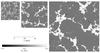 |
Fig. 6 Horizontal slices of Bz near the surface from Runs A4v, B2v, and C2v with different box sizes. The physical scale is shown in the legend. |
3.2. Imposed vertical field
Pronounced effects of the negative effective magnetic pressure have been found in the case of an imposed vertical field in studies where turbulence is forced (e.g. Brandenburg et al. 2013, 2014; Losada et al. 2014); see also Fig. 5. This occurs because a vertical field, contrary to a horizontal one, is not advected by the resulting downflow, i.e. there is no potato sack effect. However, as the downflow removes gas from the upper layers, the pressure decreases, which results in a return flow that draws with it more vertical field. This can lead to field amplification to a strength that exceeds the equipartition field strength in the top layers; see Brandenburg et al. (2013) for numerical simulations in isothermal stratified turbulence. In the above-mentioned studies the field concentrations often form a spot-like structure because the ratio between the domain size and forcing scale is sufficiently large (e.g. Brandenburg et al. 2013, 2014; Losada et al. 2014).
In the top row of Fig. 5 we show visualizations of the vertical magnetic field Bz, velocity uz, and temperature T from a depth of 0.6 Mm for Run C1v with an imposed vertical field of 230 G. We note that there are now three large patches, the largest exceeding 20 Mm in diameter, where positive Bz of the order of 3 kG is found. Line plots through two of the patches (two bottom panels of Fig. 5) show that the magnetic field exceeds the local equipartition field strength by a factor of more than ten because convection is nearly completely suppressed in regions of strong magnetic fields. The temperature within the magnetic structures at the depth of 0.6 Mm is reduced by roughly 2000 K, which is within the observed range for sunspots. We also find that the structures penetrate almost the entire depth of the layer; see the second and third rows of Fig. 5. The temperature is affected mostly near the surface, whereas in the deeper layers the difference to the ambient atmosphere is 1–2 orders of magnitude smaller than near the surface. The structures are qualitatively similar to those seen in forced turbulence simulations with poor scale separation where they are caused by NEMPI; see Fig. 17 of Brandenburg et al. (2014). This result is also reminiscent of early work of Tao et al. (1998), who found similar behaviour in large aspect ratio convection simulations, although at much smaller Rayleigh numbers and weaker density stratification.
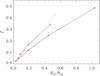 |
Fig. 7 Magnetic field redistribution factor (the relative areas in which vertical fields exceeding the equipartition value, Bz>Beq) in runs with vertical fields from Sets A (black), B (red), and C (blue). The dotted lines are proportional to Beq. |
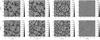 |
Fig. 8 From left to right: vertical velocity uz from depths 18, 12, 6.0, and 0.5 Mm from a hydrodynamical run C00 (top row) and a run with imposed vertical field C1v (bottom row). The velocity is given in units of km s-1. |
Representative results of the vertical field near the surface from the three domain sizes with comparable imposed fields of the order of 0.5 kG are shown in Fig. 6. We find that the size of the structures increases from roughly 5 Mm to 20 Mm as the domain size is increased from 34 Mm to 96 Mm. In addition, the field topology changes from a web-like network of strong fields in Run A4v with the smallest domain size to one with more isolated structures in Run C2v for the largest physical size. A possible explanation is that the equipartition field is smaller in Run A4v than in the other two runs (Fig. 2) and that the magnetic field has a greater effect on the flow. A similar transition from isolated magnetic structures for relatively weak fields to a network-like structure for intermediate field strengths has previously been reported by e.g. Tao et al. (1998) and Tian & Petrovay (2013). We have not explored such strong fields as Tian & Petrovay (2013); this would induce small-scale convection throughout the domain, as seen in the flux concentrations in the rightmost panel of Fig. 6.
The magnetic field redistribution factor (the relative areas in which vertical field exceeds the equipartition value) is roughly proportional to the imposed field strength; see Fig. 7. This result follows from the conservation law for the total magnetic flux, B0Ŝ = BeqŜ1 + (Ŝ−Ŝ1)Bres, where Ŝ is the total area and Ŝ1 is the area of the strong field (about the equipartition field), and Bres ≪ Beq is the final weak magnetic field (much smaller than the equipartition field). This yields f = Ŝ1/Ŝ ∝ B0/Beq.
As in the case of the imposed horizontal field, we find here for the vertical field that the large-scale contribution indicative of magnetic flux concentrations, increases as the imposed field strength is increased; see Table 2. The growth of the maximum, however, is significantly less steep in the vertical field case, especially in Sets B and C. In Set C, increases by only 20 per cent when the imposed field increases fourfold.
Given that the negative effective magnetic pressure is capable of producing downflows in ways similar to thermal convection, an interesting question is whether there are any noticeable differences between downflows produced with and without magnetic fields; Fig. 8 shows a comparison between the two (Runs C00 and C1v). For horizontal fields we show above that in both cases there are downflows, but it is not clear whether they are significantly affected by the presence of flux concentrations. Here, the most pronounced difference occurs immediately in the top layer; we see large-scale patches with almost vanishing velocity in the areas where strong magnetic fields are present. Some extended patches are also still seen at a depth of z = 6 Mm, but they are now subdominant compared with the narrower downdrafts. However, in deeper layers (below z = 12 Mm) the flow structure is similar in the two cases, except that in the case with magnetic field the flow patterns are somewhat smoother. A similar effect of dynamo-generated magnetic fields on the small-scale flow structure has been noted by Hotta et al. (2015).
We find that the magnetic concentrations tend to appear in regions where large-scale convective downflows occur; see Fig. 9 where the temporally averaged vertical magnetic field is shown along with the similarly averaged flows from Run C1v. The large-scale fields were extracted by temporally averaging over ten snapshots of the simulation data, each separated by 4.5 h. The horizontal scale of the large-scale cells is roughly 40−50 Mm, and they span the entire vertical extent of the domain. Flows at these scales correspond to supergranulation in the Sun. The fact that the flux concentrations are situated at the vertices of the large-scale convection pattern suggests that their origin is the flux expulsion mechanism proposed by Clark (1965) and Weiss (1966).
3.3. Effective magnetic pressure
In our study we measure the effective magnetic pressure in order to clarify the role of NEMPI in the formation of inhomogeneous magnetic structures in turbulent convection. Below we define the effective magnetic pressure and describe the method of its measurement. The total turbulent stress, including the contributions of Reynolds and Maxwell stresses is given by  (23)where δij is the Kronecker tensor and the superscript “(f)” refers to contributions from the fluctuations. The turbulent stress is split into two contributions that are either independent of (
 ) or dependent on (
 ) the mean field. Their difference
  is due to the mean magnetic field and can be parametrized in the form
  (24)where ĝi is the unit vector along the direction of gravity. Furthermore, qs represents the contribution of turbulence to the mean magnetic tension and qp is the corresponding contribution to the mean magnetic pressure. Finally, qg refers to the anisotropic contribution to the mean turbulent pressure owing to gravity. The effective magnetic pressure (the sum of turbulent and non-turbulent contributions to the large-scale magnetic pressure) is related to qp via
  (25)where
  .
.
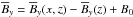
We compute qp by performing a reference simulation without an imposed field to find and a set of simulations with a mean field to determine for a given field strength. Using Eq. (24) in the x direction we find that it is sufficient to measure  , from which we obtain
  (26)This expression agrees with that used in earlier work (Losada et al. 2014).
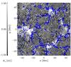 |
Fig. 9 Temporally averaged vertical magnetic field (black and white contours), horizontal flows (black and white arrows), and downflows exceeding 250 m s -1 (blue contours) at a depth of 6 Mm in Run C1v. |
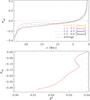 |
Fig. 10 Top panel: effective magnetic pressure |


Our measurements of the effective magnetic pressure  detected negative values in the bulk of the convection zone, roughly consisting of 80% of the deepest parts. In the uppermost 20% of the domain is always positive; see the representative result in Fig. 10 from Run C2v. The effective magnetic pressure in the middle regions of the layer between depths 2.3 and 7.0 Mm for all the runs in Set A are shown in the top panel of Fig. 11. In the present convection set-ups, the equipartition field strength is almost a constant throughout the layer and causes the curves in Fig. 11 to appear roughly as vertical lines, especially for weak imposed fields. Taking data from the same depths in runs with different B0 show a trend which is very similar to that seen in forced turbulence with a negative for weak magnetic fields and positive when the imposed field approaches equipartition; see the lower panel of Fig. 11.
The growth rate of NEMPI is proportional to the derivative of with respect to the mean magnetic field strength: 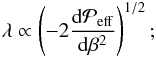 (27)see Kemel et al. (2013) for an imposed horizontal field and Brandenburg et al. (2014) for an imposed vertical one. We find that in most of our simulations the derivative of the effective magnetic pressure with respect to β2 is positive (i.e.
  ) almost everywhere in the convection layer; see the representative result from Run C2v in the lower panel of Fig. 10. In the runs with the strongest imposed vertical fields
  is negative in the lower parts of the convection zone. In Runs B3v and C3v this regime covers roughly half of the depth of the layer. The difference between the current simulations and the density-stratified forced turbulence models is that in our case the equipartition strength of the field is almost constant in the bulk of the convection zone (lower panel of Fig. 2), whereas in the latter
  . Therefore, β varies relatively little in the bulk, which is where
  . Furthermore, the derivative has the wrong sign for the excitation of NEMPI. We have not tried to devise a situation where the derivative would be suitable for instability, although this could perhaps be achieved by using imposed or dynamo-generated fields that vary with height.
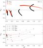 |
Fig. 11 Top panel: mean effective magnetic pressure as a function of β2 for the runs in Set A with vertical (black) and horizontal (red) imposed fields for z in the range 2.3 Mm ≤ z ≤ 7.0 Mm. Lower panel: |
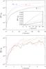 |
Fig. 12 Top panel: normalized Fourier amplitudes |


In addition to a negative derivative , the scale separation ratio of turbulence needs to be sufficiently large for the excitation of NEMPI. DNS of forced turbulence (Brandenburg et al. 2011, 2013) show that, to excite NEMPI, the scale separation ratio between the forcing scale and the size of the box should be larger than 15. Unlike the case of forced turbulence where the forcing scale can be chosen as desired, the dominant scale of turbulence in convection has to be estimated from the non-linear outcome of the instability. This can be achieved by finding the peak of the power spectrum of velocity. Convection is known to generate large-scale circulations that are considered large-scale structures rather than turbulence (e.g. Elperin et al. 2002, 2006). Thus, we first extract the fluctuating part, u′, by subtracting the average velocity obtained by adding five snapshots separated by roughly half a large-scale convective turnover time. We show power spectra of the fluctuating velocity at four depths for Run C1v in Fig. 13. We also show a comparison with the spectra from the full velocity field, showing that the power at large scales is significantly reduced. Near the surface and at a depth of 6 Mm, we find that the spectra peak at kHρ ≈ 0.1 and 1, respectively. In the deeper layers, the peak is found near kHρ ≈ 2, which is of the same order of magnitude as in Kemel et al. (2013). A similar estimate is also found for the near-surface layers from the power spectra of the vertical velocity; see the lower panel of Fig. 13. This is in contradiction with the estimate obtained from the Taylor microscale, i.e. kωHρ (Eq. (16)), which is typically an order of magnitude higher than kmax corresponding to the peak of the fluctuating velocity spectra. In contrast to earlier lower resolution simulations (e.g. Cattaneo & Hughes 2006; Käpylä et al. 2008), we find a clear inertial range appearing at intermediate scales in the deeper layers.
Previous work on NEMPI has shown evidence of an intermediate phase during which the magnetic field at large scales (characterizing the large-scale structures) grows exponentially. This was possible to see by isolating the large-scale magnetic field through appropriate Fourier filtering. In contrast, the total magnetic field, which includes the small-scale magnetic field, grows linearly in time, which is expected when turbulence acts on the applied magnetic field through tangling. The exponential evolution of the large-scale field was taken as evidence for the existence of a large-scale instability. To check whether similar evidence can be produced here as well, we study the early evolution of the largest scale Fourier components of the vertical magnetic field near the surface of Run C1v; see Fig. 12. However, it turns out that we do not find clear evidence of exponential growth for any wavenumber. The data is more consistent with linear growth suggesting that the structure formation is related to tangling of the field by large-scale convection. The lower panel of Fig. 12 shows the comparison of the two largest scale Fourier modes of By in Run A3h and a corresponding run without backreaction to the flow. In the latter case NEMPI cannot occur as the field is passive and does not contribute to turbulent pressure. We find no significant difference in the growth of the large-scale modes in these cases. This suggests that even though we find a negative contribution to the effective magnetic pressure in Run A3h, NEMPI is not excited in the simulation. We conclude that the lack of clear exponential growth of the structures in all the runs suggests that even though the sign of is favourable to NEMPI in some cases, the instability is not excited.
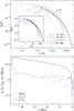 |
Fig. 13 Top panel: power spectra of the fluctuating velocity from four horizontal planes as indicated in the legend in Run C1v. The horizontal wavenumber is made non-dimensional by multiplying with the density scale height Hρ at the same depth. The dashed line shows the slope for Kolmogorov k− 5/3 scaling. The inset shows a comparison of power spectra of the full velocity field (dashed lines) and the fluctuating velocity from which the temporal average is removed (solid lines) from depths 6 Mm (blue) and 18 Mm (black). Bottom panel: wavenumbers corresponding to Taylor microscale (black solid line; see Eq. (16)), and the peaks of the fluctuating velocity power spectra (red dashed) and the fluctuating vertical velocity (blue dash-dotted) spectra as functions of depth and normalized by Hρ. |
In an earlier study, Kitiashvili et al. (2010) attribute the growth of magnetic structures to vortical flows at the vertices of convection cells. They also state that “usually the process starts at one of the strongest vortices”. We note that in the simulations of Kitiashvili et al. (2010) the aspect ratio of the box is close to unity. Compared to our runs with aspect ratio four, we find that only a few large-scale convection cells are present in the deep layers; see Fig. 8. This suggests that most likely only a single large-scale convection cell exists in the simulations of Kitiashvili et al. (2010). This is not obvious from the flows at the surface where several vortical downflows, which are all connected to the same large-scale downflow at deep layers, can be identified. Thus, in their case a single downflow plume is likely dominating the dynamics and concentrating the magnetic field, which is consistent with the interpretation in terms of flux expulsion.
4. Conclusions
We demonstrate that stratified turbulent convection leads to concentrations of magnetic field from an initially uniform field. The area that these concentrations occupy in the volume is roughly proportional to the imposed field strength. We also show that the average size of the structures increases with the box size when the imposed field strength is kept constant. The strength of magnetic structures at large scales is linearly proportional to the imposed field for horizontal fields. For imposed vertical fields we find the same dependency for the smallest domain size, whereas in larger domains the maximum approaches a constant value. We also find a negative contribution to the effective magnetic pressure, which is in agreement with earlier studies of turbulent convection (Käpylä et al. 2012a, 2013). However, the magnetic field in the concentrations does not grow exponentially at any wavenumber, but is consistent with linear growth. This indicates that the formation of magnetic concentrations is not associated here with an instability like NEMPI. We find that the magnetic concentrations appear in regions where downflows associated with large-scale, i.e. supergranular, convection occur. This process is more commonly known as flux expulsion (Clark 1965; Weiss 1966; Galloway et al. 1977; Tao et al. 1998). However, the role of turbulence in such flux expulsion is not yet clear. We note that this process is distinct from the magnetic pumping effect (e.g. Nordlund et al. 1992; Tobias et al. 1998; Ossendrijver et al. 2002), which is related to the inhomogeneity of turbulence and leads to an effective advection of the large-scale magnetic fields down the gradient of turbulence intensity (e.g. Krause & Rädler 1980). This process cannot promote the growth of magnetic flux concentrations, but can lead to downward pumping of the large-scale magnetic fields.
There are several reasons why the current simulations – whose density stratifications are an order of magnitude higher than in our earlier studies – are unable to excite NEMPI. The excitation of NEMPI requires a negative sign of the derivative of the effective magnetic pressure with respect to the large-scale magnetic field. In many cases in our simulations this derivative was positive, i.e. unfavourable for NEMPI. In addition, it is possible that the separation of scales between the system size and the turbulent scale is insufficient (which in our simulations is only between 1–2 when measured from the peak of the velocity power spectra, while in forced turbulence the scale separation ratio of around 15 is needed to observe NEMPI). Furthermore, convection in the current set-up always tends to develop at the largest possible scale, which increases as the domain size increases, and which dominates the generation of magnetic concentrations. If this tendency carries over to the Sun, a naive assumption is that giant cells of the order of 200 Mm should be present and that they would dominate the process of magnetic structure formation. Although detection of giant cells in the Sun has been reported (e.g. Hathaway et al. 2013), local time-distance helioseismology appears to indicate a gaping discrepancy between the Sun and current global simulations in that the latter produce significantly too much power at large scales (Hanasoge et al. 2012). Local ring-diagram helioseismology, on the other hand, gives much larger convective velocities (Greer et al. 2015). Nevertheless, at least circumstantial evidence suggests that a new paradigm of convection could be needed. A possible candidate is the concept of “entropy rain” (Spruit 1997; Brandenburg 2015) where only a thin top layer of the convection zone, perhaps only a few Mm, is Schwarzschild unstable and the rest of the layer is mixed by strong downflows plunging deep into the stably stratified interior. In such a scenario the largest scale excited by convection would be of the order of the depth of the Schwarzschild unstable layer, and thus very much smaller than in the current simulations where typically the whole domain is unstable. This would eliminate giant cells and also increase the scale separation drastically, perhaps enabling NEMPI. However, devising numerical models capturing this idea is challenging.
Another future step is to study the formation of magnetic structures in turbulent stratified convection from the dynamo-generated field similar to that of a forced turbulence (Mitra et al. 2014; Jabbari et al. 2014, 2015).
Online material
Movie of Fig. 4 Access Supplementary Material
Movie of Fig. 5 Access Supplementary Material
Acknowledgments
We thank the referee for useful comments. The simulations were performed using the supercomputers hosted by CSC – IT Center for Science Ltd. in Espoo, Finland, who are administered by the Finnish Ministry of Education. Special Grand Challenge allocation NEMPI12 is acknowledged. Financial support from the Academy of Finland grants No. 136189, 140970, 272786 (PJK), and 272157 to the ReSoLVE Centre of Excellence (PJK, MJK), as well as the Swedish Research Council grants 621-2011-5076 and 2012-5797, and the Research Council of Norway under the FRINATEK grant 231444 are acknowledged.
References
- Arlt, R., Sule, A., & Rüdiger, G. 2005, A&A, 441, 1171 [NASA ADS] [CrossRef] [EDP Sciences] [Google Scholar]
- Augustson, K., Brun, A. S., Miesch, M., & Toomre, J. 2015, ApJ, 809, 149 [Google Scholar]
- Brandenburg, A. 2005, ApJ, 625, 539 [Google Scholar]
- Brandenburg, A. 2015, ArXiv e-prints [arXiv:1504.03189] [Google Scholar]
- Brandenburg, A., Kleeorin, N., & Rogachevskii, I. 2010, Astron. Nachr., 331, 5 [NASA ADS] [CrossRef] [Google Scholar]
- Brandenburg, A., Kemel, K., Kleeorin, N., Mitra, D., & Rogachevskii, I. 2011, ApJ, 740, L50 [NASA ADS] [CrossRef] [Google Scholar]
- Brandenburg, A., Kemel, K., Kleeorin, N., & Rogachevskii, I. 2012, ApJ, 749, 179 [NASA ADS] [CrossRef] [Google Scholar]
- Brandenburg, A., Kleeorin, N., & Rogachevskii, I. 2013, ApJ, 776, L23 [NASA ADS] [CrossRef] [Google Scholar]
- Brandenburg, A., Gressel, O., Jabbari, S., Kleeorin, N., & Rogachevskii, I. 2014, A&A, 562, A53 [NASA ADS] [CrossRef] [EDP Sciences] [Google Scholar]
- Candelaresi, S., & Brandenburg, A. 2013, Phys. Rev. E, 87, 043104 [NASA ADS] [CrossRef] [Google Scholar]
- Cattaneo, F., & Hughes, D. W. 2006, J. Fluid Mech., 553, 401 [NASA ADS] [CrossRef] [Google Scholar]
- Cheung, M. C. M., Rempel, M., Title, A. M., & Schüssler, M. 2010, ApJ, 720, 233 [NASA ADS] [CrossRef] [Google Scholar]
- Choudhuri, A. R., Schussler, M., & Dikpati, M. 1995, A&A, 303, L29 [NASA ADS] [Google Scholar]
- Choudhuri, A. R., Chatterjee, P., & Jiang, J. 2007, Phys. Rev. Lett., 98, 131103 [Google Scholar]
- Clark, Jr., A. 1965, Phys. Fluids, 8, 644 [NASA ADS] [CrossRef] [Google Scholar]
- Dikpati, M., & Charbonneau, P. 1999, ApJ, 518, 508 [NASA ADS] [CrossRef] [Google Scholar]
- Dikpati, M., & Gilman, P. A. 2006, ApJ, 649, 498 [NASA ADS] [CrossRef] [Google Scholar]
- Elperin, T., Kleeorin, N., Rogachevskii, I., & Zilitinkevich, S. 2002, Phys. Rev. E, 66, 066305 [NASA ADS] [CrossRef] [Google Scholar]
- Elperin, T., Kleeorin, N., Rogachevskii, I., & Zilitinkevich, S. S. 2006, Bound.-Layer Meteor., 119, 449 [NASA ADS] [CrossRef] [Google Scholar]
- Featherstone, N. A., & Miesch, M. S. 2015, ApJ, 804, 67 [NASA ADS] [CrossRef] [Google Scholar]
- Galloway, D. J., Proctor, M. R. E., & Weiss, N. O. 1977, Nature, 266, 686 [NASA ADS] [CrossRef] [Google Scholar]
- Ghizaru, M., Charbonneau, P., & Smolarkiewicz, P. K. 2010, ApJ, 715, L133 [NASA ADS] [CrossRef] [Google Scholar]
- Greer, B. J., Hindman, B. W., Featherstone, N. A., & Toomre, J. 2015, ApJ, 803, L17 [NASA ADS] [CrossRef] [Google Scholar]
- Guerrero, G., & Käpylä, P. J. 2011, A&A, 533, A40 [NASA ADS] [CrossRef] [EDP Sciences] [Google Scholar]
- Hanasoge, S. M., Duvall, T. L., & Sreenivasan, K. R. 2012, PNAS, 109, 11928 [Google Scholar]
- Hathaway, D. H., Upton, L., & Colegrove, O. 2013, Science, 342, 1217 [NASA ADS] [CrossRef] [Google Scholar]
- Haugen, N. E. L., & Brandenburg, A. 2006, Phys. Fluids, 18, 075106 [NASA ADS] [CrossRef] [Google Scholar]
- Hotta, H., Rempel, M., Yokoyama, T., Iida, Y., & Fan, Y. 2012, A&A, 539, A30 [NASA ADS] [CrossRef] [EDP Sciences] [Google Scholar]
- Hotta, H., Rempel, M., & Yokoyama, T. 2014, ApJ, 786, 24 [NASA ADS] [CrossRef] [Google Scholar]
- Hotta, H., Rempel, M., & Yokoyama, T. 2015, ApJ, 803, 42 [NASA ADS] [CrossRef] [Google Scholar]
- Jabbari, S., Brandenburg, A., Losada, I. R., Kleeorin, N., & Rogachevskii, I. 2014, A&A, 568, A112 [NASA ADS] [CrossRef] [EDP Sciences] [Google Scholar]
- Jabbari, S., Brandenburg, A., Kleeorin, N., Mitra, D., & Rogachevskii, I. 2015, ApJ, 805, 166 [NASA ADS] [CrossRef] [Google Scholar]
- Käpylä, P. J., Korpi, M. J., & Brandenburg, A. 2008, A&A, 491, 353 [NASA ADS] [CrossRef] [EDP Sciences] [Google Scholar]
- Käpylä, P. J., Brandenburg, A., Kleeorin, N., Mantere, M. J., & Rogachevskii, I. 2012a, MNRAS, 422, 2465 [NASA ADS] [CrossRef] [Google Scholar]
- Käpylä, P. J., Mantere, M. J., & Brandenburg, A. 2012b, ApJ, 755, L22 [NASA ADS] [CrossRef] [Google Scholar]
- Käpylä, P. J., Brandenburg, A., Kleeorin, N., Mantere, M. J., & Rogachevskii, I. 2013, in IAU Symp. 294, eds. A. G. Kosovichev, E. de Gouveia Dal Pino, & Y. Yan, 283 [Google Scholar]
- Käpylä, P. J., Käpylä, M. J., & Brandenburg, A. 2014, A&A, 570, A43 [NASA ADS] [CrossRef] [EDP Sciences] [Google Scholar]
- Kemel, K., Brandenburg, A., Kleeorin, N., Mitra, D., & Rogachevskii, I. 2012a, Sol. Phys., 280, 321 [NASA ADS] [CrossRef] [Google Scholar]
- Kemel, K., Brandenburg, A., Kleeorin, N., & Rogachevskii, I. 2012b, Astron. Nachr., 333, 95 [NASA ADS] [CrossRef] [Google Scholar]
- Kemel, K., Brandenburg, A., Kleeorin, N., Mitra, D., & Rogachevskii, I. 2013, Sol. Phys., 287, 293 [NASA ADS] [CrossRef] [Google Scholar]
- Kitchatinov, L. L., & Mazur, M. V. 2000, Sol. Phys., 191, 325 [NASA ADS] [CrossRef] [Google Scholar]
- Kitiashvili, I. N., Kosovichev, A. G., Wray, A. A., & Mansour, N. N. 2010, ApJ, 719, 307 [NASA ADS] [CrossRef] [Google Scholar]
- Kleeorin, N., & Rogachevskii, I. 1994, Phys. Rev. E, 50, 2716 [NASA ADS] [CrossRef] [Google Scholar]
- Kleeorin, N. I., Rogachevskii, I. V., & Ruzmaikin, A. A. 1989, Sov. Astron. Lett., 15, 274 [NASA ADS] [Google Scholar]
- Kleeorin, N. I., Rogachevskii, I. V., & Ruzmaikin, A. A. 1990, Sov. Phys. JETP, 70, 878 [Google Scholar]
- Kleeorin, N., Mond, M., & Rogachevskii, I. 1993, Phys. Fluids B, 5, 4128 [NASA ADS] [CrossRef] [Google Scholar]
- Kleeorin, N., Mond, M., & Rogachevskii, I. 1996, A&A, 307, 293 [NASA ADS] [Google Scholar]
- Krause, F., & Rädler, K.-H. 1980, Mean-field Magnetohydrodynamics and Dynamo Theory (Oxford: Pergamon Press) [Google Scholar]
- Losada, I. R., Brandenburg, A., Kleeorin, N., & Rogachevskii, I. 2014, A&A, 564, A2 [NASA ADS] [CrossRef] [EDP Sciences] [Google Scholar]
- Mitra, D., Brandenburg, A., Kleeorin, N., & Rogachevskii, I. 2014, MNRAS, 445, 761 [NASA ADS] [CrossRef] [Google Scholar]
- Nordlund, A., Brandenburg, A., Jennings, R. L., et al. 1992, ApJ, 392, 647 [NASA ADS] [CrossRef] [Google Scholar]
- Ossendrijver, M., Stix, M., Brandenburg, A., & Rüdiger, G. 2002, A&A, 394, 735 [NASA ADS] [CrossRef] [EDP Sciences] [Google Scholar]
- Parker, E. N. 1955, ApJ, 121, 491 [NASA ADS] [CrossRef] [Google Scholar]
- Passos, D., Charbonneau, P., & Miesch, M. 2015, ApJ, 800, L18 [NASA ADS] [CrossRef] [Google Scholar]
- Rempel, M. 2005, ApJ, 622, 1320 [NASA ADS] [CrossRef] [Google Scholar]
- Rempel, M., Schüssler, M., Cameron, R. H., & Knölker, M. 2009a, Science, 325, 171 [NASA ADS] [CrossRef] [PubMed] [Google Scholar]
- Rempel, M., Schüssler, M., & Knölker, M. 2009b, ApJ, 691, 640 [NASA ADS] [CrossRef] [Google Scholar]
- Rogachevskii, I., & Kleeorin, N. 2007, Phys. Rev. E, 76, 056307 [NASA ADS] [CrossRef] [Google Scholar]
- Schad, A., Timmer, J., & Roth, M. 2013, ApJ, 778, L38 [NASA ADS] [CrossRef] [Google Scholar]
- Spruit, H. 1997, Mem. Soc. Astron. It., 68, 397 [NASA ADS] [Google Scholar]
- Stein, R. F., & Nordlund, Å. 2012, ApJ, 753, L13 [Google Scholar]
- Stix, M. 2002, The Sun: An Introduction (Berlin: Springer) [Google Scholar]
- Tao, L., Weiss, N. O., Brownjohn, D. P., & Proctor, M. R. E. 1998, ApJ, 496, L39 [NASA ADS] [CrossRef] [Google Scholar]
- Tian, C., & Petrovay, K. 2013, A&A, 551, A92 [NASA ADS] [CrossRef] [EDP Sciences] [Google Scholar]
- Tobias, S. M., Brummell, N. H., Clune, T. L., & Toomre, J. 1998, ApJ, 502, L177 [NASA ADS] [CrossRef] [Google Scholar]
- Warnecke, J., Losada, I. R., Brandenburg, A., Kleeorin, N., & Rogachevskii, I. 2013, ApJ, 777, L37 [NASA ADS] [CrossRef] [Google Scholar]
- Warnecke, J., Käpylä, P. J., Käpylä, M. J., & Brandenburg, A. 2014, ApJ, 796, L12 [NASA ADS] [CrossRef] [Google Scholar]
- Warnecke, J., Losada, I. R., Brandenburg, A., Kleeorin, N., & Rogachevskii, I. 2016, A&A, in press, DOI: 10.1051/0004-6361/201525880 [Google Scholar]
- Weiss, N. O. 1966, Proc. Roy. Soc. London Ser. A, 293, 310 [Google Scholar]
- Yadav, R. K., Gastine, T., Christensen, U. R., & Reiners, A. 2015, A&A, 573, A68 [NASA ADS] [CrossRef] [EDP Sciences] [Google Scholar]
- Zhao, J., Bogart, R. S., Kosovichev, A. G., Duvall, Jr., T. L., & Hartlep, T. 2013, ApJ, 774, L29 [NASA ADS] [CrossRef] [Google Scholar]
All Tables
All Figures
|
Fig. 1 Comparison of the stratifications of our three hydrodynamic runs A00 (black), B00 (red), and C00 (blue) showing density a), pressure b), the density (solid lines) and pressure scale heights (dashed lines) c), correlation length lcorr = 2π/kωd), and specific entropy e). |
| In the text | |
|
Fig. 2 Profiles of horizontally averaged rms velocity urms (top, a)) and equipartition magnetic field Beq (bottom, b)) from the same runs as in Fig. 1 in units of m s-1 and kG, respectively. |
| In the text | |
|
Fig. 3 a) Mean magnetic field component |
| In the text | |
|
Fig. 4 Vertical magnetic field Bz near the surface at a depth of 0.6 Mm from representative snapshots of Runs C2h (left panel), C3h (middle), and C4h (right). The magnetic field scale is clipped at ± 3 kG in each panel. The maximum field strengths obtained are of the order of 5 kG. Animation associated with Run C4h can be found online and at http://research.ics.aalto.fi/cmdaa/group-Movies.shtml. |
| In the text | |
|
Fig. 5 Top row: vertical magnetic field Bz, vertical velocity uz, and temperature T, respectively, at z = 0.6 Mm for Run C1v. The second and third rows show vertical cuts from cuts through y = 15.9 Mm and y = −5.8 Mm. In the rightmost panels we show the |
| In the text | |
|
Fig. 6 Horizontal slices of Bz near the surface from Runs A4v, B2v, and C2v with different box sizes. The physical scale is shown in the legend. |
| In the text | |
|
Fig. 7 Magnetic field redistribution factor (the relative areas in which vertical fields exceeding the equipartition value, Bz>Beq) in runs with vertical fields from Sets A (black), B (red), and C (blue). The dotted lines are proportional to Beq. |
| In the text | |
|
Fig. 8 From left to right: vertical velocity uz from depths 18, 12, 6.0, and 0.5 Mm from a hydrodynamical run C00 (top row) and a run with imposed vertical field C1v (bottom row). The velocity is given in units of km s-1. |
| In the text | |
|
Fig. 9 Temporally averaged vertical magnetic field (black and white contours), horizontal flows (black and white arrows), and downflows exceeding 250 m s -1 (blue contours) at a depth of 6 Mm in Run C1v. |
| In the text | |
|
Fig. 10 Top panel: effective magnetic pressure |
| In the text | |
|
Fig. 11 Top panel: mean effective magnetic pressure as a function of β2 for the runs in Set A with vertical (black) and horizontal (red) imposed fields for z in the range 2.3 Mm ≤ z ≤ 7.0 Mm. Lower panel: |
| In the text | |
|
Fig. 12 Top panel: normalized Fourier amplitudes |
| In the text | |
|
Fig. 13 Top panel: power spectra of the fluctuating velocity from four horizontal planes as indicated in the legend in Run C1v. The horizontal wavenumber is made non-dimensional by multiplying with the density scale height Hρ at the same depth. The dashed line shows the slope for Kolmogorov k− 5/3 scaling. The inset shows a comparison of power spectra of the full velocity field (dashed lines) and the fluctuating velocity from which the temporal average is removed (solid lines) from depths 6 Mm (blue) and 18 Mm (black). Bottom panel: wavenumbers corresponding to Taylor microscale (black solid line; see Eq. (16)), and the peaks of the fluctuating velocity power spectra (red dashed) and the fluctuating vertical velocity (blue dash-dotted) spectra as functions of depth and normalized by Hρ. |
| In the text | |
Current usage metrics show cumulative count of Article Views (full-text article views including HTML views, PDF and ePub downloads, according to the available data) and Abstracts Views on Vision4Press platform.
Data correspond to usage on the plateform after 2015. The current usage metrics is available 48-96 hours after online publication and is updated daily on week days.
Initial download of the metrics may take a while.