| Issue |
A&A
Volume 588, April 2016
|
|
|---|---|---|
| Article Number | A48 | |
| Number of page(s) | 20 | |
| Section | Extragalactic astronomy | |
| DOI | https://doi.org/10.1051/0004-6361/201527730 | |
| Published online | 16 March 2016 | |
Asymmetric mass models of disk galaxies
I. Messier 99
1 Univ. Bordeaux, LAB, UMR 5804, 33270 Floirac, France
e-mail: This email address is being protected from spambots. You need JavaScript enabled to view it.
2 CNRS, LAB, UMR 5804, 33270 Floirac, France
3 INAF–Osservatorio Astrofisico di Arcetri, Largo Enrico Fermi 5, 50125 Firenze, Italy
4 Institut d’Astrophysique de Paris, CNRS & Université Pierre & Marie Curie (UMR 7095), 98 bis Bd Arago, 75014 Paris, France
5 Mullard Space Science Laboratory, University College London. Dorking, Surrey, RH5 6NT, UK
Received: 11 November 2015
Accepted: 6 January 2016
Abstract
Mass models of galactic disks traditionally rely on axisymmetric density and rotation curves, paradoxically acting as if their most remarkable asymmetric features, such as lopsidedness or spiral arms, were not important. In this article, we relax the axisymmetry approximation and introduce a methodology that derives 3D gravitational potentials of disk-like objects and robustly estimates the impacts of asymmetries on circular velocities in the disk midplane. Mass distribution models can then be directly fitted to asymmetric line-of-sight velocity fields. Applied to the grand-design spiral M 99, the new strategy shows that circular velocities are highly nonuniform, particularly in the inner disk of the galaxy, as a natural response to the perturbed gravitational potential of luminous matter. A cuspy inner density profile of dark matter is found in M 99, in the usual case where luminous and dark matter share the same center. The impact of the velocity nonuniformity is to make the inner profile less steep, although the density remains cuspy. On another hand, a model where the halo is core dominated and shifted by 2.2−2.5 kpc from the luminous mass center is more appropriate to explain most of the kinematical lopsidedness evidenced in the velocity field of M 99. However, the gravitational potential of luminous baryons is not asymmetric enough to explain the kinematical lopsidedness of the innermost regions, irrespective of the density shape of dark matter. This discrepancy points out the necessity of an additional dynamical process in these regions: possibly a lopsided distribution of dark matter.
Key words: galaxies: kinematics and dynamics / galaxies: fundamental parameters / galaxies: structure / galaxies: spiral / galaxies: individual: Messier 99 (NGC 4254) / dark matter
© ESO, 2016
1. Introduction
Rotation curves and surface density profiles of galactic disks are the observational pillars most models of extragalactic dynamics are based on. Rotation curves are needed to constrain the total mass distribution, the parameters of dark matter haloes, or the characteristics of modified Newtonian dynamics, while surface density profiles are helpful to constrain the structural parameters of disks and bulges, and generate the velocity contributions of luminous matter essential to mass models. As the density and rotation velocity profiles are axisymmetric by construction, mass models implicitly assume that the rotational velocity is only made of uniform circular motions. Though attractive for its simplicity, this approach remains a reductive exploitation of velocity fields and multiwavelength images of stellar and gaseous disks, which are information rich. In particular, it prevents one from measuring the rotational support through perturbations (spiral arms, lopsidedness, etc.), which are obviously the most striking features of galactic disks. In an era of conflict between observations and expectations from cold dark matter (CDM) simulations, the cusp-core controversy (see the review of de Blok 2010, and references therein; but see Governato et al. 2010), it appeared fundamental to assess the impact of such perturbations on the shape of rotation curves, and more generally on mass models and density profiles of dark matter.
This is the reason why efforts have been made to determine the kinematical asymmetries inferred by perturbations or to model the effects of dynamical perturbations. In the former case, Franx et al. (1994) and Schoenmakers et al. (1997) initiated the derivation of high-order harmonics with first-order kinematical components from gaseous velocity fields. They argued that kinematical Fourier coefficients are useful to constrain deviations from axisymmetry and the nature of dynamical perturbations. Using that technique, Gentile et al. (2005) concluded, for instance, that the kinematical asymmetries in the Hi velocity field of a dwarf disk presenting a core-dominated dark matter halo (DDO 47) could likely originate from a spiral structure. However, their amplitudes were not high enough to account for the velocity difference expected between the CDM cusp and the cored halo preferred by the rotation curve fittings. In the second case, Spekkens & Sellwood (2007) proposed to fit a bisymmetric model of bar-like/oval distortion to the Hα velocity field of another low-mass spiral galaxy (NGC 2976) and argued that negligible high-order Fourier motions in velocity fields do not necessarily imply that the bisymmetric perturbation is negligible, and that the rotation curve should be similar to the underlying circular motions only if the departures from circularity remain small. These authors also showed that the inner slope of the rotation curve of NGC 2976 is likely affected by the bar-like perturbation. Numerical simulations of barred disks arrived at a similar conclusion about the impact of the bar on the inner shape of rotation curves (Valenzuela et al. 2007; Dicaire et al. 2008). Randriamampandry et al. (2015) performed numerical simulations to determine a corrected rotation curve for another barred galaxy (NGC 3319), free from the perturbing motions induced by the bar. While these simulations demonstrate it is possible to hide cuspier DM distributions into artificial cored distributions under the effect of stellar bars, they perfectly illustrate the difficulty of performing mass models and constraining the shape of dark matter density profiles from observations of barred galaxies. Other numerical models based on closed-loop orbits showed that shallow kinematics and core-like haloes could actually be explained by cuspy triaxial distributions of dark matter viewed with particular projection angles (Hayashi & Navarro 2006). Finally, other studies focused on extracting in Hi spectra the line-of-sight (l.o.s.) velocity components supposed to trace the axisymmetric rotational velocities better than the components based on more usual intensity-weighted means (Oh et al. 2008). Applied to two dark matter dominated disks, NGC 2366 and IC 2574, which are prototypes of galaxies whose dark matter density conflicts with the cosmological cusp, this method yielded steeper rotation curves in the inner disk regions. However, the velocity differences with the intensity-weighted mean velocity curve were not sufficient to reconcile the observation with the CDM cusp.
In this context, in this article we propose a new approach to model the mass distribution of disk galaxies. Our strategy goes beyond the decomposition of rotation curves and fully exploits the bidimensional distribution of luminous matter, thus the asymmetric nature of stellar and gaseous disks. Our approach determines the 3D gravitational potential of any disk-like mass component through hyperpotentials theorized by Huré (2013). It then derives the corresponding circular velocity map in the disk midplane, which allows us to determine where and to which extent the circular motions should deviate from axisymmetry. A 2D mass distribution model can then be directly fitted to a l.o.s. velocity field, by adding the 2D velocity contributions from luminous baryons to that from the missing matter. The impacts of the velocity asymmetries on the mass models and structure of dark matter haloes can then been investigated by comparing with results obtained with the axisymmetric mass models.
We apply that methodology to a prototype of unbarred, spiral galaxy Messier 99, whose general properties are presented in Sect. 2. The axisymmetric mass model of the high-resolution rotation curve of M 99 is detailed in Sect. 3. This section also presents a more elaborated axisymmetric mass model, fitted directly to a high-resolution velocity field of M 99. The basis of the derivation of the 3D gravitational potentials for luminous matter is described in Sect. 4, which also presents the inferred gravitational potentials, accelerations, and circular velocities for the contributions from the stellar, atomic, and molecular gas disks of M 99. The meaning of these asymmetric outputs is discussed in Sect. 5. We then perform asymmetric mass distribution models of M 99 (Sect. 6), and compare them to the axisymmetry-based models of Sect. 3. The conclusions for M 99 and the prospects of our new strategy for galactic dynamics are finally given in Sect. 7.
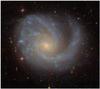 |
Fig. 1 Composite SDSS gri-image of the grand-design spiral galaxy M 99. North is up; east is left. The image size is 7′ × 6.3′. |
2. The grand-design spiral galaxy Messier 99
2.1. A brief presentation
We selected the galaxy Messier 99 (M 99 hereafter) because it is a SAc type disk harboring a very prominent spiral structure (Fig. 1). Located in the Virgo Cluster (adopted distance of 17.1 Mpc, Freedman et al. 1994), observing M 99 is a good opportunity to benefit from high-sensitivity and high-resolution multiwavelength observations of the stellar disk and interstellar medium. The integrated Hα profile from data of Chemin et al. (2006) has a width at 20% of the maximum Hα peak of 216 km s-1. Combined with a small disk inclination (20°, Makarov et al. 2014), this implies a massive galaxy with most of rotation velocities greater than 245 km s-1. This makes it an ideal target to study the structure and kinematics of the disk in detail and to test our new mass modeling strategy.
The spiral structure is asymmetric. A one-arm mode dominates the Hi disk (Phookun et al. 1993; Chung et al. 2009), while the stellar distribution exhibits more than one single arm (Fig. 1). Phookun et al. (1993) proposed a scenario where the Hi arm is triggered by gas infalling and winding on the disk, resulting from a tidal encounter. Based on numerical simulations, Vollmer et al. (2005) mimic the asymmetric disk and perturbed Hi kinematics by a flyby of a massive companion, coupled with ram pressure stripping from the Virgo intracluster medium (ICM). These authors argued that M 99 is entering the Virgo cluster for the first time. Further numerical models of Duc & Bournaud (2008) also explained the origin of the large-scale Hi tail, which apparently connects M 99 to VIRGOHI21, a 108 M⊙ Hi cloud wandering in the Virgo ICM (Minchin et al. 2007), by a tidal interaction that was with another candidate companion than in Vollmer et al. (2005). In principle, mass distribution models should only be carried out with targets supposedly in dynamical equilibrium. The possibly infalling Hi mass of ~ 108 M⊙ only represents ~2% of the total neutral gas mass of M 99, and about 0.2% of the total luminous mass (Sect. 3). This should be not enough to affect the large-scale dynamics of M 99. Furthermore, ram pressure stripping predominantly affects the outskirts of the neutral atomic gas component, not the inner, densest regions of the gaseous disk of M 99.
2.2. High-resolution Hα kinematics
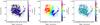 |
Fig. 2 Hα integrated emission, velocity field, and velocity dispersion map of M 99 (from left to right, respectively). |
Optical long-slit and resolved observations also revealed perturbed kinematics of the ionized gas disk of M 99 (Phookun et al. 1993; Kranz et al. 2001; Chemin et al. 2006). In particular, Kranz et al. (2001) argues for the presence of a possible stellar bar that would impact the Hα kinematics in the inner 1.5 kpc. Asymmetric motions have also been clearly evidenced along the Hα spiral arms (Phookun et al. 1993; Chemin et al. 2006), as well as a lopsided Hα velocity field (Chemin et al. 2005b). The kinematical data we use to model the mass distribution of M 99 are from the 3D spectroscopy survey of Virgo cluster galaxies by Chemin et al. (2005a, 2006). In their catalog of Hα velocity fields of bright Virgo spiral and irregular disks, the Fabry-Perot observations of M 99 have angular and spectral samplings of 1.6′′ (130 pc at the adopted distance) and ~ 8.2 km s-1. The Hα velocity field of Chemin et al. (2006) resulted from an adaptive binning and a spatial interpolation of the Hα datacube, following prescriptions given in Daigle et al. (2006). We did not use these interpolated data but an improved version of the binned datacube of Chemin et al. (2006), where new bins are now made of a unique pixel located at the barycenter of initial bins. Every bin has thus an equal angular size, in accordance with the kinematical analysis of many other Hα Fabry-Perot velocity fields (Epinat et al. 2008a,b). Figure 2 shows the revisited integrated Hα emission, velocity, and dispersion velocity fields of M 99. We restricted the Hα kinematics to R = 11.5 kpc, which corresponds to a distribution of 9002 velocity pixels. This allowed us to derive accurate velocity and velocity dispersion profiles. Beyond the optical size of the stellar disk, the Hi kinematics is too scattered to infer useful kinematical information.
3. Axisymmetric mass modeling of M 99
A traditional axisymmetric mass model consists in decomposing a rotation curve into contributions from luminous baryons (stellar and gaseous disks, bulge, etc.) and dark matter. The fitting procedure yields fundamental scale parameters for the hidden mass component, and eventually a factor that enables the scaling of luminosities into surface densities for stars (the mass-to-light ratio, M/L). This section details the rotation curve decomposition, which we refer to as the 1D axisymmetric case hereafter, as the rotation velocity only depends on one angular scale, which is the galactocentric radius.
This section also envisages a second strategy, where the axisymmetric modeling is carried out directly from the velocity field. The motivation for this is, first, that circular motions are expected to dominate the kinematics and, since rotation curves stem from velocity fields, one may logically perform mass models with 2D resolved data instead of 1D curves. The second motivation is that the development of a pipeline that makes fittings in 2D is mandatory for the new asymmetric methodology discussed from Sects. 4 to 6. The most natural way to understand the impact of the asymmetries on the mass models is, thus, to fit to the Hα velocity field of M 99 2D velocity models built under axisymmetry assumptions. In short, one cannot directly compare the results from the decomposition of the rotation curve with those presented in Sect. 6 for the asymmetric fittings of the velocity field. One needs an intermediate step between them, which we refer to as the 2D axisymmetric case hereafter. Though the data to be fitted are not totally axisymmetric because of the evident signatures of, for example, spiral arms, we nonetheless call this 2D case axisymmetric because the individual contributions from dark matter, stars, and gas are distributed axisymmetrically.
This section is therefore organized as a traditional axisymmetric mass model of a galactic disk. We first derive the rotation curve of M 99 and estimate the asymmetric drift contribution, and then we present multiwavelength observations needed to infer the mass surface density profiles and the velocity contributions of the stellar and interstellar matter. The results of the mass modeling are then discussed to investigate which dark matter halo shape is more appropriate. In addition, we discuss the 2D axisymmetric modeling.
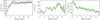 |
Fig. 3 Left and middle: profiles of tangential and radial velocity of M 99. Shaded area indicates the 1σ rms from the fittings. A green solid line represents the fitting for the whole disk, while blue dotted and red crossed circles are respectively the results for the approaching and receding sides fitted separately. Right panel: Hα velocity dispersion of M 99. Symbols represent the observed dispersion; the dashed line is a smooth model of the observation used to derive the asymmetric drift. |
3.1. Tangential and radial velocities in M 99
As the mass distribution modeling first needs a rotation curve, the 3D velocity space (vR,vθ,vz) is deduced from fitting to the Hα velocity field of M 99 the following model:  (1)where vl.o.s is the l.o.s. velocity, vsys and i are the systemic velocity and the inclination of the M 99 disk, and θ is the azimuthal angle in the deprojected orbit. In the axisymmetric approach, these velocities are assumed uniform, i.e. only dependent on R. The azimuthal velocity is the rotation curve. The vR and vz components are usually omitted in kinematical studies because they are generally assumed to be negligible. As seen below, it is the case for vR but since one of our goals is to study the impact of the radial motions on the mass modeling, we decided to fit them. Deriving vθ with or without vR does not impact the shape or amplitude of the tangential component. Then, a problem in leaving vz free in Eq. (1) is that it should exhibit artificial variations if the galaxy has a kinematical lopsidedness. The reason for this is that the systemic velocity must be naturally impacted by a lopsidedness (see Appendix B), but since variations of vsys are not allowed here, the vzcosi term absorbs the kinematical signature of lopsidedness. As both the gravitational potential of luminous matter and the Hα kinematics of M 99 are lopsided (Sect. 4.2 and Appendix B), the best solution to avoid such artificial vz variations is thus to assume vz = 0 hereafter. Other face-on, grand-design spirals of similar star formation activity to M 99 are known to have negligible vertical motions (e.g., NGC 628, Kamphuis & Briggs 1992).
Since the Hα gas is well confined in the optical disk that is not warped, we have not allowed vsys, i, the position angle of the disk major axis (Γ) and the coordinates of the dynamical center to vary with radius. We chose θ = 0° aligned with the semimajor axis of the receding side of the galaxy disk. We used an inclination of 20°, which is the one of the stellar disk, i.e. the photometric value. This value differs from the kinematical value of 31° ± 6° derived in Chemin et al. (2006). The photometric value is more appropriate for the mass modeling than larger inclinations (see Sect. 3.3). Nonlinear Levenberg-Marquardt fittings were performed with uniformly weighted velocities. We found vsys = (2398 ± 0.5) km s-1 and Γ = (67 ± 0.5)°. The kinematical center appears slightly offset from the photometric center (peak of the stellar density). However that difference is not significant owing to the measured uncertainties (see also Chemin et al. 2006). For simplicity, we adopt the photometric center as the kinematical center. These results are in very good agreement with Chemin et al. (2006). The Hα systemic velocity agrees well with the centroid of the integrated Hα profile from our dataset (2392 km s-1) or the value found by Chung et al. (2009) from the integrated Hi profile of M 99 (2395 km s-1). Then, we derived vR and vθ with all other parameters fixed at these adopted values. We chose an adaptive angular sampling with a ring size of at least 2.5′′ (well larger than the seeing of the observations) and with a minimum number of 30 pixels per ring to ensure good quality fits. With these rules, radial bins are fully uncorrelated.
Figure 3 shows the resulting profiles of vθ and vR, whose values are reported in Table C.1 of Appendix C. The rotation curve is regular. It shows a peak at R ~ 3 kpc, which roughly corresponds to the radius equivalent to 2.2 times the stellar disk scalelength (see Sect. 3.2), and a flat part at larger radii (vθ ~ 270 km s-1). This rotation curve is consistent with the Hα measurements presented in Phookun et al. (1993), Kranz et al. (2001), and Chemin et al. (2006) after scaling at similar inclinations. We also verified the good consistency with CO kinematics from Leroy et al. (2009). The rotation curves for the approaching and receding halves of the Hα disk have also been fitted separately. They are asymmetric in the inner 2 kpc, and around 3−3.5 kpc. This is one of the signatures of the kinematical lopsidedness of M 99. The Very Large Array (VLA) data did not allow us to perform a reliable tilted-ring model of the Hi velocity field for R> 11.5 kpc. The scatter of the Hi kinematics is indeed too large to consider an outer Hi rotation curve, and constrain the parameters of a disk warping, if any warp exists in M 99. This has nonetheless no consequence on the results presented hereafter because Hi densities are small and the gravitational impact of the atomic gas disk is negligible in the overall mass budget.
The rotation of M 99 is clockwise, assuming trailing spiral arms. With this rule, positive vR (negative, respectively) corresponds to motions radially oriented inward (outward). As a consequence, the fitted profile presents globally inward radial motions in M 99, except in the inner R = 2.7 kpc, between R = 4.9 kpc and R = 5.9 kpc and locally at R = 3.7 kpc and R = 6.9 kpc, which are consistent with vR directed outward. Beyond R ~ 10 kpc, the scatter of the radial component becomes larger, though this scatter is mainly consistent with a velocity directed outward. The formal error from the fittings are small at these radii and remain negligible relative to the amplitude of vR.
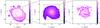 |
Fig. 4 Surface density maps for the atomic gas, stellar and molecular gas disks of M 99 (from left to right, respectively). Densities (in M⊙ pc-2) are shown in a decimal logarithmic scale. |
It is expected that the observed tangential velocity of the kinematical tracer differs from its circular velocity because of asymmetric drift. Starting from Eq. (4.227) of Binney & Tremaine (2008), and assuming that random motions drives the gas pressure, an isotropic dispersion ellipsoid, and that the product vRvz is independent of z, the circular velocities, vc, are deduced from the tangential motions by 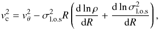 (2)where σl.o.s is the observed l.o.s. dispersion and ρ is the total (atomic+molecular) mass volume density that can be replaced by the surface density Σ if we also assume a constant disk thickness. The atomic and molecular gas densities are those presented in Sect. 3.2. The Hα velocity dispersion profile, corrected from instrumental broadening, is shown in Fig. 3 and listed in Appendix C. The mean dispersion is 20 km s-1 for a standard deviation of ~2 km s-1, which is comparable to values found for many other star-forming galaxies of similar morphology and mass (Epinat et al. 2010; Kam et al. 2015). The profile variations of the density and dispersion remain too small to imply a significant gas asymmetric drift. Equation (2) yields an almost constant pressure support, well represented by an average value ⟨ vc−vθ ⟩ ~ 1 km s-1. Because of this minor correction relatively to vθ, asymmetric drift is neglected hereafter. Such values are fully consistent with results found for other dwarf or massive disk galaxies (de Blok & Bosma 2002; Gentile et al. 2007; Swaters et al. 2009; Dalcanton & Stilp 2010; Westfall et al. 2011; Martinsson et al. 2013).
3.2. Stellar and gaseous surface densities
The mass models need velocity contribution from luminous matter. We have considered individual contributions from a molecular gas disk (mol), an atomic gas disk (atom), a stellar disk (⋆,D), and a stellar bulge (⋆,B). The corresponding velocity components are deduced from mass surface densities.
The molecular gas disk surface densities are from CO 1−0 mm observations of Rahman et al. (2011) from the Combined Array for Research in Millimeter-wave Astronomy array, at an angular resolution of 4.3′′. The CO 0-th moment map has been translated to H2 surface densities using a conversion factor of 1.8 × 1020 cm-2 (K km s-1)-1. The H2 gas mass is ~ 5 × 10⁹ M⊙. The atomic gas disk surface densities come from the Very Large Array Hi survey of Virgo Cluster galaxies by Chung et al. (2009), originally from Phookun et al. (1993), at an angular resolution of ~25′′. Using the adopted distance, the Hi gas mass is ~ 5 × 10⁹ M⊙, which is thus the same as the H2 mass. The total mass density maps for the atomic and molecular contributions are finally obtained by multiplying the Hi and H2 densities by the usual factor of 1.37 to take the contribution of elements that are heavier than hydrogen into account.
The stellar mass surface densities are estimated using the method of Zibetti et al. (2009), based on the pixel-by-pixel comparison of optical and near-infrared (NIR) colors with a suite of stellar population synthesis models. Zibetti et al. (2009) and Zibetti (2009) provide details of the image reduction and signal-to-noise enhancement via adaptive smoothing, which allows one to extract accurate (error < 0.05 mag) surface brightness at each pixel in g, i, and H-bands, respectively, and, in turn, g−i,i−H colors. We compute the same colors for a set of 150 000 composite stellar population synthesis (SPS) models with variable star formation histories (exponentially declining plus random bursts), metallicities, and two-component dust attenuations as in Charlot & Fall (2000), following the prescriptions of da Cunha et al. (2008). The models are binned in the g−i, i−H space and the median M/L in H-band is computed for each bin. For any given pixel, the measured g−i and i−H colors select the bin in the model libraries and the corresponding M/L is assigned to the pixel. By multiplying the H-band surface brightness with this M/L, we obtain the stellar mass surface density. With respect to the SPS library adopted in Zibetti et al. (2009), the only difference is that the base of simple stellar populations (SSP) is not the so-called CB07 version of the Bruzual & Charlot (2003, BC03) models, but the 2012 updated version of the original BC03 SSPs1. In fact, in recent years, many observations have shown that models with a very strong contribution by TP-AGB stars (e.g., Maraston 2005, CB07) fail to reproduce the optical-NIR spectral energy distribution of galaxies in the low- to intermediate-redshift Universe (e.g., Kriek et al. 2010; Zibetti et al. 2013; Melnick & De Propris 2014), while models with a more moderate TP-AGB contribution (e.g. BC03) work better. This motivates our decision to opt for BC03 SSPs. The M/L in H −band estimated with TP-AGB light models are typically 0.1−0.2 up to 0.3 dex higher than estimated with TP-AGB heavy models (see Fig. 3 of Zibetti et al. 2009). The 2012 update of BC03 introduces some improvements in the treatment of the stellar remnant, which results in larger M/L by roughly 10% for old stellar populations. The pixel scale of the stellar mass map is 1.6′′. The stellar mass of M 99 is ~ 4.2 × 10¹⁰ M⊙. In total, it yields a luminous mass of 5.2 × 10¹⁰ M⊙.
 |
Fig. 5 Left: mass surface density profile of stars in M 99. A bulge-disk decomposition model (green solid line) to the observed profile (symbols) is seen, as well as bulge and disk components (red dashed lines). Right: axisymmetric mass distribution model of M 99. The rotation curve is represented with filled symbols, and its model with an orange solid line. Contributions from the stellar bulge and disk are shown with red dashed lines, from the atomic and molecular gas disks with blue dash-dotted lines, and from the dark matter component with green open symbols. The dark matter model is the best-fit NFW halo whose parameters are given in Table D.1. |
The images have been deprojected with constant kinematical parameters as function of radius, using i = 20° and a position angle of 67°. We set the x> 0 axis of our deprojected frame to be coincident with to the semimajor axis of the receding half of the disk. We have also assumed that all luminous mass contributions share the same dynamical center, that is, fixed at the position of the photometric center. Figure 4 shows the resulting surface density maps. The prominent spiral structure of M 99 is observed at all angular scales with more obvious spiral patterns for the molecular gas and stellar components. The outer stellar spiral arm (x< 0) coincides well with the outer spiral arm of the atomic gas disk.
3.3. Luminous and dark matter velocity contributions
The following model is fitted to a kinematical observable  (3)where vDM the circular velocity contribution from the missing mass (dark matter, or DM), and vlum that from the total luminous mass, given by
 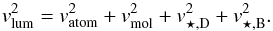 (4)Equations (3) and (4) assume tracers at centrifugal balance, which is probably not totally verified because of the disk asymmetries. In our 1D axisymmetric approach, azimuthally averaged surface density profiles have been derived from the resolved density maps of Sect. 3.2. The stellar mass surface density profile is shown in Fig. 5. The bulge component has a mass of ~ 4.7 × 10⁹ M⊙ and follows an exponential law of central density and scalelength (Σ0,h) ~ (7450 M⊙ pc-2, 0.3 kpc). The main stellar contribution comes from a disk with a scalelength of h⋆ = 1.7 kpc and a central density of ~1800 M⊙ pc-2. The density profile is better modeled with the addition of an outer truncated component having a scalelength of ~ 20 kpc for a central density of ~40 M⊙ pc-2.
The circular velocity derives from the radial acceleration gR, as  , assuming a pressureless mass component. The circular velocity contribution v⋆,B of the bulge has been derived from the bulge density assuming a spherical bulge. The circular velocity contribution of the stellar disk v⋆,D has been deduced from a residual density profile obtained by subtracting the bulge density to the total stellar density profile. The main disk and outer components are thus contained in this residual profile, and we do not differentiate between both disk parts hereafter. The vertical density law of the stellar disk cannot be measured directly for an almost face-on galaxy like M 99. We have assumed it follows a sech-squared law (van der Kruit & Searle 1981) with a constant scaleheight of ~ 0.35 kpc. This value corresponds to 20% of the M 99 disk scalelength, following results found for edge-on disks (e.g., Yoachim & Dalcanton 2006). The vertical structure of gaseous disks is less observationally constrained than for stellar disks. We considered that the gaseous disks are thin structures of negligible scaleheight.
Figure 5 shows the individual velocity profiles. One sees that the stellar disk dominates the other luminous contributions, except in the inner kpc where it is comparable with the bulge contribution. We emphasize that using an inclination of, for example, ~30° as in Chemin et al. (2006) would systematically make the stellar contribution overestimate the rotation curve in the inner disk regions. Unless the stellar mass of M 99 has been significantly overestimated or the asymmetric drift has been significantly underestimated, using a lower kinematical inclination than those given by Phookun et al. (1993), Kranz et al. (2001), or Chemin et al. (2006) is the best solution to reconcile the Hα kinematics with the photometric inclination and the results from models of stellar populations synthesis.
The larger concentration of molecular gas in the inner disk causes vmol to dominate over vatom; the latter velocity steadily increases toward the outer regions and peaks at a radius larger than the last point of the Hα rotation curve. The radius of the peak of the stellar disk contribution R = 2.2h⋆ = 3.7 kpc coincides well with that of the inner peak of the rotation curve. This confirms our finding of a small scalelength for the stellar disk of M 99. At this radius, if the velocity contribution of the stellar disk dominates the rotation curve at a level of more than 75% (v⋆,D/vθ> 75%) for galaxies similar in morphological type to M 99, then the stellar disk is said to be maximum (Sackett 1997). We measure a stellar disk velocity fraction of 67% at R = 3.7 kpc. Also, taking the bulge contribution into account leads to a stellar fraction of 72% and all luminous matter gives a velocity fraction of 78%. The stellar disk of M 99 is thus not maximum, and the luminous baryons are barely maximum with this definition. This confirms that dark matter is a significant contribution to the total mass budget of M 99, as often observed in nearby spirals (e.g., Bershady et al. 2011; Westfall et al. 2011; Martinsson et al. 2013).
The velocity contribution of dark matter is assumed to be that of a spherical halo (r = R) whose center coincides with that of the disk of luminous matter (hereafter centered-halo case). The DM halo models we fitted are the Einasto model (EIN hereafter), the cuspy model inferred from cosmological simulations (the Navarro-Frenk-White model; NFW hereafter), and the core-dominated model (pseudoisothermal sphere; PIS hereafter).
The mass density profile of the Einasto model (Navarro et al. 2004) is defined as  (5)Here r-2 is the characteristic scale radius at which the density profile has a logarithmic slope of −2, ρ-2 is the scale density at that radius, and n is a dimensionless index that shapes the profile. The circular velocity implied by the Einasto model is
  (6)where
  is the incomplete gamma function and ξ = 2n(r/r-2)1 /n (Cardone et al. 2005; Mamon & Łokas 2005; Retana-Montenegro et al. 2012). This three-parameter model has the flexibility to choose between a steep, intermediate, or shallow density profile, depending on the value of the index. At fixed characteristic density and radius, models with small (large) indices correspond to shallow (steep, respectively) inner density profiles (Chemin et al. 2011).
The density of the NFW profile (Navarro et al. 1997) is  (7)corresponding to a circular velocity profile
  (8)where x = r/r200. The parameter r200 is the virial radius derived where the density equals 200 times the critical density
  for closure of the Universe; and η = cx, where c is the concentration of the DM halo. We fixed the Hubble constant at the value found by the Planck Collaboration H0 = 68 km s-1 Mpc-1 (Planck Collaboration XIII 2015). The two parameters are the scale velocity v200 and the halo concentration c. The NFW halo is said to be cuspy because the density scales as r-1 in the center, which is steeper compared with the density profile of the pseudoisothermal sphere
  (9)which thus tends to the constant value ρ0 in the core region of the halo. This model is therefore referred as a core. The parameter rc is the characteristic core radius of the halo. The density profile implies a circular velocity
  (10)Each of vEIN, vNFW, or vPIS replaces vDM in Eq. (3).
3.4. Mass distribution modeling
The rotation curve is the observable for the 1D modeling, while the Hα velocity field of M 99 has been fitted in the 2D case. For that, a modeled l.o.s. velocity map is built following Eqs. (1) and (3) with fixed kinematical parameters, using axisymmetric velocity contributions from dark matter, molecules, atoms, and stars. In practice, it is the bidimensional tangential velocity only that is modified in Eq. (1), as the parameters of dark matter vary while fitting the observation. However, we have built two l.o.s. projections: with and without fixed radial motions. The modeling without vR assumes vR = 0, while that with fixed vR uses the axisymmetric profile derived in Sect. 3.1. Modeling with noncircular motions is referred as the 2D+vR case hereafter. Though not perfect, as vR is not dynamically motivated unlike vθ, the 2D+vR case remains a simple method to estimate the global impact of noncircular motions in the dynamical modeling and the inner shape of the dark matter density.
The SPS modeling of Zibetti et al. (2009) already provide the scaling of the stellar mass. Our models only have those of the DM component as free parameters. Fittings were thus carried out with 52 d.o.fs (9000, respectively) for the NFW and PIS models, and 51 d.o.fs (8999) for the EIN model in the 1D axisymmetric case (2D). As in Sect. 3.1., we used uniform weightings for the 2D models. Rotation curve decomposition often uses normal weightings that are the inverse of the squared uncertainties on rotation velocities, Δvθ. We defined  as the quadratic sum of the formal error from the rotation curve fitting with a systematic error (half the velocity difference between the approaching and receding disk halves). The error distribution is not Gaussian, which prevents us from using normal weightings. We thus used the number of points per radial bin as the weighting function of velocities. Though this is not homogeneous to the 2D weighting function, it turned out to be the most appropriate way to account for a distribution of velocities in the rotation curve comparable to the pixel distribution in the velocity field.
Appendix D (Table D.1) reports the fitted parameters of the different halo models. The quoted parameter errors correspond to the formal 1σ error from the fittings. Both 1D and 2D fittings are correct and yield parameters in good agreement within the errors. The 2D modeling yields more constrained parameters than for the 1D case. We also note the degeneracy for the halo parameters of the Einasto model. This degeneracy is partially raised in the 2D case, as the Einasto index is about 2.5 times more constrained. We base the analysis upon the Akaike Information Criterion (AIC; Akaike 1974) to compare the different halo models, following Chemin et al. (2011). The criterion is defined by AIC = 2N + χ2, where N is the number of parameters to be fitted by the modeling (N = 2 for NFW and PIS, N = 3 for EIN). Since the AIC involves both the χ2 and the number of parameters, an AIC test is then appropriate to compare models that are not nested and do not have a similar numbers of parameters, such as the NFW, PIS, and EIN forms. An AIC test cannot be invoked to rule out a specific model, but instead helps us to decide which model is more likely than others. Chemin et al. (2011) applied this criterion to analyze rotation curves of disks from the Hi Nearby Galaxy Survey (Walter et al. 2008; de Blok et al. 2008) and found that in most of configurations the Einasto model is an improvement with respect to the NFW and PIS models. As the smaller the AIC, the more likely one model with respect to another, we then compared two models by deriving the difference between their respective AIC (Table D.2). Reporting AIC differences explains why Table D.1 does not list the χ2 of each fitting.
The Einasto and NFW cusps are found to be the most likely models, compared with the pseudoisothermal sphere. We estimate a DM density slope at the first point of the rotation curve R = 0.27 kpc of −0.88 ± 0.37 for the 1D case (−0.87 ± 0.33 for the 2D case) for the Einasto model, thus slightly shallower than for the NFW cusp (~−1). The AIC difference between the NFW and Einasto cusps implies that the three-parameter model is more likely. However, it is difficult to judge the real pertinence of this result because of the degeneracy of the Einasto model parameters. The best-fit 1D mass model with the NFW halo is shown in Fig 5. Results for the 2D model that take the radial motions into account follow the same trends, and an inner DM slope of −0.84 ± 0.31 is deduced for the EIN model. This slope is only marginally shallower than for the model without vR. The noncircular radial motions have a negligible impact on shaping the DM density profile of M 99, at least within this axisymmetry approach.
4. Dynamical asymmetries of M 99 luminous matter
The benefit from a 2D analysis should become more interesting if the velocity contribution from luminous matter could stick to the asymmetric reality of the luminous matter. The objective of this section is thus to describe the methodology and products of the asymmetric approach (gravitational potentials, radial, and tangential forces), and in particular the resolved circular velocity contribution of luminous matter to be used by the 2D asymmetric modeling presented in Sect. 6.
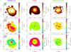 |
Fig. 6 Gravitational potential (Φ), tangential, and radial acceleration (gθ and gR, respectively) maps of the disks of the atomic, molecular gas, and stellar components of M 99. These maps are for the z = 0 kpc midplane. The axisymmetric contribution from the bulge potential is not included in the stellar disk component. |
4.1. Methodology
The major difference between the axisymmetric case and the asymmetric approach is that we need to derive the 3D, asymmetric gravitational potential of luminous baryons beforehand. We thus computed the potential in Cartesian coordinates (x,y,z), which enables us to derive both radial and azimuthal forces at any desired z. This can be derived independently for each stellar or gaseous contribution. The gravitationtal potential Φ of the mass distribution is in principle deduced from the convolution of the volume mass density by the Green function, namely 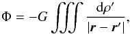 (11)where G is the gravitational constant. However, the Green function written by 1/ | r−r′ | = [(x−x′)2 + (y−y′)2 + (z−z′)2] − 1/2, is well known to diverge at each point where x = x′, y = y′ and z = z′. This function renders any direct estimate of Φ inaccurate and generally encourages modelers to incorporate a softening length to bypass the divergence. Here, we use the new formalism presented in Huré (2013) who showed that the Newtonian potential is exactly reproduced by using an intermediate scalar function ℋ, namely
  . In 3D, this hyperpotential is written as
 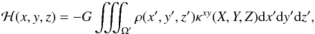 (12)with X = x−x′, Y = y−y′ and Z = z−z′. The κ function is a hyperkernel defined by
 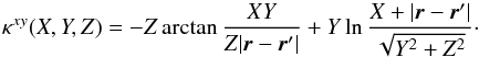 (13)This approach is particularly simple and efficient for 2D or 3D distributions since ℋ is, in contrast to Φ, the convolution of the surface or volume density with a regular, finite amplitude kernel. The methodology thus does not make use of a softening length in the derivation of the potential. In practice, this convolution is performed using the second-order trapezoidal rule and the mixed derivatives are estimated at the same order from centered finite differences. Furthermore, the volume density of the tracer are deduced from a surface density map, considering that the vertical density follows a sech-squared or exponential law of constant scaleheight with radius. The precision of these schemes is sufficient for the present purpose.
The volume density of gas and stars were derived using their respective surface densities (Sect. 3.2 and Fig. 4). Similar to the axisymmetric case, we considered a sech-squared law, using a scaleheight of 0.35 kpc for the vertical variation of the density of the stellar disk, and that the molecular and atomic gas disks have negligible scaleheights. Once the 3D gravitational potential of a tracer is derived, the azimuthal and radial components of the gravitational acceleration are obtained from gθ = −∇θΦ and gR = −∇RΦ, respectively. From the 3D products, we can extract the gravitational potential, radial, and tangential accelerations in the galaxy midplane (z = 0 kpc). This is necessary to fit the observed kinematics of ionized gas that is assumed to lie in that plane.
4.2. Asymmetric gravitational potentials and accelerations
Figure 6 shows the midplane potential maps for the stellar and gaseous disk components of M 99. As we are primarily interested in the asymmetric components, the axisymmetric potential of the bulge is not represented here (see Fig. A.3 for its radial profile). We only show pixels for which the density is strictly positive for each component, as these are the most important regions for the analysis. Beyond the observable extent of each disk, the potential well decreases smoothly with radius and has no interesting features that deserve to be shown.
The absolute strength of the potential is observed to increase from the atomic gas, to the molecular gas, and finally to the stellar component. As expected, none of the potentials show pure axial symmetry, as they exhibit lopsided and spiral-like features. To quantify the nonaxisymmetric perturbations, we have modeled the gravitational potentials via a series of harmonics, as detailed in Appendix A. We find that the stellar and gaseous potentials are indeed lopsided (m = 1 mode), and exhibit spiral structures (m = 2 modes) and other less prominent m = 3 perturbations. We also find that the stellar potential is not barred and that the lopsidedness dominates the amplitude of the stellar perturbations in the inner disk region, while it totally dominates those in the disk of atomic gas. We derived the azimuthally averaged ratios of total perturbed against unperturbed potentials to summarize the importance of the perturbations. These ratios are written as ⟨ ∑ m ≠ 0Φm(R)cos(m(θ−θm(R))/Φ0(R) ⟩ θ = ⟨ Φ(R,θ) ⟩ θ/ Φ0(R)−1, following Eq. (A.1) and are shown in Fig. 7. They show that the degree of perturbation significantly increases with decreasing mass density. The stellar potential is preferentially less disturbed in regions where perturbations of the molecular gas potential are stronger. On overall average, we find that the gravitational potential is disturbed at the level of ~ 10% for the atomic gas component, ~ 5% for molecules, and ~ 2% for stars. The addition of the bulge potential to the axisymmetric part of the potential of the stellar disk only marginally modifies the ratio of perturbations for the stellar component.
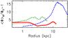 |
Fig. 7 Fraction (in %) of the perturbed potential to the unperturbed potential for luminous matter in M 99. The red solid (dotted) line is for the stellar disk (stellar bulge+disk) potential, green dashed line for the molecular gas disk, and blue dash-dotted line for the atomic gas disk. |
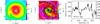 |
Fig. 8 Left: circular velocity field for the contribution of luminous matter only. Middle: zoom in the inner 4 kpc with contours representing the emission from molecular gas. A dashed circle shows the location of R = 2.2h⋆ = 3.7 kpc, where h⋆ is the stellar disk scalelength. Right: variation of velocity with azimuth at R = 3.7 kpc. Open circles represent the velocities of four points inside, down- and upstream of the spiral arms, indicated with white filled circles in the middle panel. The dashed line is the axisymmetric value. The velocity scale of the left axis is for luminous matter only, while that of the right axis takes an additional contribution from dark matter into account. |
Figure 6 also shows the tangential and radial accelerations in the midplane. The most important results are that gθ is far from negligible and then that gR and gθ are strongly asymmetric. The morphology of the gR maps is intrinsically linked to spiral structures in the density and potential maps, while structures in the gθ maps differ markedly from the other density, potential, and radial acceleration fields. The sign of gR is almost exclusively negative except on the trailing sides of the gaseous arms, principally at R = 1−2.5 kpc and R = 4.5−5 kpc. Interestingly, these radii coincide or are very close to regions where the ionized gas has its radial motion outwardly directed (Sect. 3.1 and Fig. 3). The (absolute) radial force increases radially in the trailing sides of the (density) spirals and reaches local maxima. Once the peak of density has been met, it decreases on the leading sides to reach local minima. As for the azimuthal acceleration, its structure is governed by striking alternations of positive and negative patterns. Basically, gθ varies rapidly through the spiral arms, admitting a minimum where the density is maximum. It also presents a large gradient in the center of the stellar disk. We estimate that the mean tangential acceleration is about 70, 300, and 3950 times smaller than the mean radial acceleration for the atomic gas, molecular gas, and stellar disk (respectively). The tangential force is thus completely negligible over the entire disk on average, but this is only due to the alternating patterns. Indeed, this is not the case anymore on small scales since gθ and gR have comparable amplitudes.
4.3. Nonuniform circular velocity
On a global scale only, circular motions can almost be considered as purely axisymmetric. However, the implication that both gθ ≠ 0 and gR are asymmetric is that the circular velocity must be nonuniform. To quantify the velocity nonuniformity, we derived the circular velocity field vlum for the total luminous matter following Eq. (4). The major difference from the axisymmetric approach is that each circular velocity contribution now depends on (x,y). That velocity field is built on a (x,y)-grid similar to the stellar component. Velocity contributions of the gaseous disks have thus been interpolated at the nodes of the stellar grid. Figure 8 shows the vlum field for the whole disk as well as in a region focusing in the inner R = 4 kpc.
The velocity field presents many spiral patterns, which are mostly caused by the perturbed stellar and molecular contributions. The map admits extrema that depend on the location with respect to the spiral arm. Basically, the velocity sharply increases on the trailing sides of the spiral arms where the density of stars and gas increases, then peaks at higher densities, to sharply decrease on the leading sides of the arms. Streaming motions observed along spiral arms of galaxies, usually identified by wiggles in contours of l.o.s. velocities, naturally find their origin in the nonuniformity of circular motions. Examples of modeled l.o.s. velocity field with apparent streaming motions are presented in Sect. 6. An example of highly nonuniform circular velocities is shown in the right panel of Fig. 8 with the azimuth-velocity diagram at R = 2.2h⋆ = 3.7 kpc. At this radius, the stellar contribution is maximum and the axisymmetric circular velocity of total luminous matter is ⟨ vlum ⟩ ~ 207 km s-1 (or 259 km s-1 when a contribution from, e.g., the best-fit NFW halo of the 2D axisymmetric case of Sect. 3.4 is included). The overall variation of velocity, 65 km s-1 (52 km s-1 with DM), is very significant; the standard deviation, which is ~ 13 km s-1 (10 km s-1), is significant as well. The sharp gradients in the trailing sides of the spiral arms for azimuths 101° to 127°, and 294° to 311° are of 54 and 59 km s-1, respectively (44 and 47 km s-1 with dark matter included). Such nonuniformity is remarkable considering the very proximity of the points (e.g., θ = 294° and 311° are separated by 1.2 kpc only).
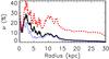 |
Fig. 9 Radial profile of the nonuniformity factor ν, defined as the maximum velocity variation with azimuth relatively to the axisymmetric velocity. The solid line is for total (luminous+dark) matter, blue dotted line for stellar and dark matter (no gas), and red dashed line for the total luminous matter (no dark matter). |
We define a nonuniformity factor, ν, as the maximum variation of circular velocity relatively to the axisymmetric circular velocity (Fig. 9). The nonuniformity factor is important in the inner disk regions. As rule of thumb, it exceeds 10% for R ≲ 2.2h⋆. with a maximum of ~ 30% (~ 40% without DM) at R = 2.5 kpc. This factor is less strong in the outer spiral arm at R ~ 10 kpc, up to a level of ~ 9% (25% without DM). For R> 12 kpc, bumps can be identified as caused by the m = 1,2,3 perturbations in the gravitational potential of the atomic gas. Here, however, ν smoothly decreases because of the dominant axisymmetric contribution of dark matter. A close inspection of the vatom, vmol, and v⋆,D maps reveals the important contribution of gas in the nonuniformity, thus in generating velocity wiggles in the M 99 spiral arms. This effect is shown with the dotted line that corresponds to the ν factor when the total gaseous component is omitted. We estimate that gas is responsible for about half of ν and the scatter of circular velocity at R = 2.2h⋆, although the stellar disk velocity contribution is larger by 100 km s-1 than that of total gas at this radius. In the R = 9−10 kpc spiral arms, atomic gas contributes by up to ~20% to ν. Self-gravity of gas is therefore not negligible in M 99, in particular, in the densest disk regions. The impact of gas could have been even more important with a higher angular resolution for the atomic gas component. Indeed, the low angular resolution of the current Hi observations has smeared out the surface density of the atomic gas, which has then likely prevented us from deriving higher velocity contrasts through arm-interarm regions, such as those evidenced within the stellar and molecular components.
5. Comparison with previous works and numerical simulations
It is important to clarify that nonuniform is not equivalent to noncircular, although both phenomena have connections as they are caused by perturbed potentials. In most kinematical studies of disk galaxies, noncircular motions are often only associated with asymmetries. This is however only part of the reality since asymmetry/nonuniformity applies both to noncircular and circular motions. Our method can only estimate the degree of nonuniformity of circular motions for M 99, however. It should also be possible to estimate this degree for the noncircular (radial) component with more advanced dynamical modeling, but this is beyond the scope of the article.
Also, the literature usually refers to circular as the axisymmetric value of the rotational motion only, while departures from that mean value are often called noncircular. This circularity-axisymmetry association turns out to be inadequate since departures from the axisymmetric velocities, such as those identified in Sect. 4.3, directly stem from the radial force as a natural response to perturbed potentials. The designation nonuniform for such departures is thus more appropriate. The interesting point for circular motions in M 99 is that nonuniformity is the rule rather than exception, whereas axisymmetry is rarely expected to occur. This is the reason why we make the difference throughout the article, on the one hand, between the axisymmetric circular and the nonuniform circular components and, on the other hand, between the noncircular and the nonuniform circular components.
The knowledge of nonuniform velocities and asymmetric radial and tangential forces in disk galaxies is not new. First, in numerical simulations, the study of asymmetric motions has been shown to be powerful to understand the response of gaseous or stellar particles to barred, spiral, or lopsided potentials, (e.g., among many articles, Combes & Sanders 1981; Athanassoula 1992; Wada 1994; Sellwood & Binney 2002; Maciejewski 2004; Bournaud et al. 2005; Quillen et al. 2011; Grand et al. 2012; Minchev et al. 2012; Renaud et al. 2013). For instance, simulations are helpful to study the radial migration of stellar particles through spiral arms and the dynamical effects of the spiral structure on radial and rotational velocities to predict signatures to be detected by kinematical samples of Galactic disk stars (Kawata et al. 2014b). Simulations can also depict the strong influence of the dynamics in a stellar bar on velocities across and along the bar axes in order to analyze the survival and merging of gaseous clouds and their implication on star formation (Renaud et al. 2015). Simulations can also show how the velocity nonuniformity prevents us from measuring the correct shape of the Milky Way rotation curve from Hi measurements (Chemin et al. 2015). Second, the nonuniformity of the tangential and radial velocity is inherent to the theory of potential perturbations (Franx et al. 1994; Rix & Zaritsky 1995; Jog 1997; Schoenmakers et al. 1997; Jog 2000, 2002; Binney & Tremaine 2008). Applications of the theory to observations has allowed the study of the elongation of galactic disk potentials (Schoenmakers et al. 1997; Simon et al. 2005) or to constrain the amplitudes of elliptical streamings and of pure radial inflows along spiral arms (Wong et al. 2004), which was made possible by a decomposition of l.o.s. velocity fields into Fourier harmonics (see Appendix B for the case of M 99). Jog (2002) predicted the signatures of galaxy lopsidedness on rotation curves. Spekkens & Sellwood (2007) also illustrated the effects of nonuniformity for a galaxy perturbed by an inner bar-like/oval distortion, but on l.o.s. motions and from a different harmonic model than in Schoenmakers et al. (1997) and Wong et al. (2004).
Then, derivations of stellar potentials from photometry have already been carried out. Zhang & Buta (2007) and Buta & Zhang (2009) determined the stellar potential for ~ 150 barred galaxies from near-infrared images to measure phase shifts between the density and potential and to constrain corotation radii. The comparison with our work remains limited as these authors restricted the analysis to 1D calculations and assumed constant mass-to-light ratios over the disks. Kranz et al. (2001) used NIR imagery with constant M/L as well to generate the gravitational potential of the stellar disk of M 99. These authors ran hydrodynamical simulations to follow the gas response to the asymmetric potential of stars and to compare with Hα kinematics. Our analysis differs from that of Kranz et al. since they proposed that the central spheroid is a stellar bar extending to about one disk scalelength; they estimated this scalelength at 36′′ or ~ 3 kpc at our adopted distance, thus about twice the value we derived. Our harmonic analysis of the stellar potential is not consistent with a bar because the phase angle of the central m = 2 perturbation varies at these radii (Fig. A.2). A comparison of dynamical asymmetries is impossible, however, as these authors have not shown radial profiles or a resolved map of the asymmetric stellar potential.
An apparent difference between theoretical and numerical modeling with our approach is that it is the tangential component that varies with azimuth in such modeling, rather than the circular velocity, while we stated that azimuthal departures from axisymmetry are those of vc. There are however striking similarities that are worth reporting. Indeed, the azimuthally periodic patterns evidenced in the vc map of M 99 are very reminiscent of those predicted for vθ by the theory or simulations for other galaxies. This implies that the circular velocity can be a good approximation for the tangential component,  . To verify this statement, we applied our methodology to a numerical simulation of a disk of similar mass and morphology as the Milky Way. Details of the simulation are described in Kawata et al. (2014b), and we have used the same snapshot as their Fig. 1. The simulation followed the evolution of the gas and stellar disks with an N-body/SPH code (GCD+; Kawata et al. 2003; Barnes et al. 2012; Kawata et al. 2013, 2014a). Figure 10 shows a strong correlation between our predicted vc and the simulated vθ of gaseous particles (seen here at, e.g., R = 5.4 and 10.8 kpc). Both velocities strongly vary as a response to the gravitational impacts of the spiral arms. Differences between vc and vθ nonetheless exist, as seen, e.g., by a slightly smaller variation of vc for R = 5.4 kpc at θ = 200−320°, or by vθ lagging (or exceeding) vc at, e.g., θ = 120−170° for R = 5.4 kpc, or θ = 200−230° for R = 10.8 kpc. These offsets are caused by particles that are losing (or gaining, respectively) angular momentum (see also Fig. 4 of Kawata et al. 2014b), and that thus have nonmarginal radial motions. The circular motion is therefore altered by noncircular motions at these locations. Other notable differences are vθ dips or peaks occurring on very small angular scales, which are not present in vc. They are disturbances of gas kinematics due to star formation and feedback processes in the simulation. Despite those irregularities, the main result is that vθ and vc are very comparable so that the 2D mass distribution models should benefit from using nonuniform circular velocities.
 |
Fig. 10 Azimuthal velocity profiles at R = 5.4 and 10.8 kpc in the simulation of the MW-like galaxy of Kawata et al. (2014b). Filled symbols are the tangential velocity of the gas component of the simulated galaxy. The green solid line is the nonuniform circular velocity predicted from the asymmetric methodology, the violet dashed line is the uniform circular motion. |
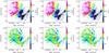 |
Fig. 11 Top: modeled velocity field of M 99 in the 2D axisymmetric, asymmetric, and asymmetric+vR cases for the Einasto halo (from left to right, respectively). Bottom: corresponding residual maps (observed minus modeled velocities). Velocity contours are from 2300 to 2500 km s-1 in step of 10 km s-1. |
6. Asymmetric mass modeling of M 99
In our 2D asymmetric approach, the variations of vθ are therefore governed by those of vc (vθ ≃ vc). The model velocity field is supposed to be that of a tracer of negligible asymmetric drift, whose assumption should hold for gas in M 99 (Sect. 3.1). Furthermore, the asymmetric dynamical modeling does not try to reproduce possible departures from circularity that are locally associated with star-forming regions and feedback, such as expanding gas shells or gas accretion from galactic fountains. This section presents the results of the asymmetric mass models using the inputs and observables decribed in the previous sections.
6.1. Impact of nonuniform circular velocities
We performed least-squares fittings of the velocity field model projected along the line of sight to the observed Hα velocity field of M 99, following Eq. (1) and with uniform weightings. As for the axisymmetric case, we fitted models with and without radial motions. The modeling with vR is hybrid between axisymmetry and asymmetry as vR is axisymmetric, unlike vθ. In this section, the spherical dark matter halo is centered on the coordinates of the center of mass of the luminous gas and stellar disks. Section 6.2 presents models with an alternative position of the dynamical center of dark matter. Results of the nonlinear minimizations are listed in Table D.1 of Appendix D and the differences of Akaike Information Criteria are given in Table D.2.
It is found that the Einasto model is more likely than the NFW cusp, which in turn is more likely than the PIS model, irrespective of the contribution from vR. This result confirms the trend observed for 2D axisymmetric modeling. The degeneracy of Einasto parameters is insignificant, in contrast with the axisymmetric results. Dark matter tends to be slightly less concentrated than in the axisymmetric case. Moreover, the derived density slope for the Einasto halo is −0.72 ± 0.27 at R = 0.27 kpc (−0.70 ± 0.26 with vR). The impact of nonuniform circular motions is therefore to yield a less cuspy halo than in the axisymmetric case. This trend goes in the same direction as the effect of noncircular motions, but at a larger extent. It seems likely that dealing with nonuniform, noncircular velocities would amplify this trend as well.
In Fig. 11, we show the velocity field of the best-fit model for the Einasto halo along with a corresponding map of residuals. For comparison, the 2D axisymmetric model of the Einasto halo is also shown. The velocity contours highlight the significant differences between both strategies. Not surprisingly, the asymmetric case exhibits velocity wiggles in the spiral arms that are not observed in the axisymmetric case. The combination of an asymmetric distribution of tangential velocities for luminous matter with a less cuspy dark matter halo has improved the modeling of the l.o.s. kinematics. We estimate that for the pixels where the residuals are lower (mainly on the leading sides of the spiral arms), the median drop in residuals is about 20% the amplitude of axisymmetry-based residuals. Other pixels have seen their residual rising (mainly on the trailing sides), but at a smaller rate (10%). Residual velocities are consequently less scattered than in the axisymmetric case. We measure a standard deviation of residuals that is smaller by up to 2 km s-1 inside 2h⋆ than in the axisymmetric case, i.e. in regions where the velocity contribution of luminous matter is the most nonuniform (Fig. 9). The improvement is also reflected by positive AICAxi.−AICAsym. differences (Table D.2), and is effective for any halo shapes.
As for the beneficial consideration of vR in the modeling, it is also verified by the AIC tests irrespective of the halo shape and of the uniformity of circular motions. Modeling has mostly been improved in regions where vR are larger (R< 1.5h⋆). This trend was expected because vR results from a prior fitting of the Hα velocity field of M 99. The remarkable effect of vR on the residuals is a motivation to mix both nonuniform circular and noncircular velocities in future dynamical works.
6.2. A shifted dark matter halo in M 99?
An important result from the Fourier analysis of the potentials was to evidence the dominance of m = 1 perturbing modes in inner regions of the stellar disk, through the entire Hi disk, and at some specific locations in the molecular disk. A detailed description of the effects of the potential perturbations on velocities in the epicycle theory has been given in Franx et al. (1994), Jog (1997), Schoenmakers et al. (1997), or Jog (2000). Schoenmakers et al. (1997) proposed that galaxy velocity fields can be decomposed into harmonics to evidence signatures of dynamical perturbations (see Eq. (B.1)). They showed that a m −order perturbation of the gravitational potential generates kinematical Fourier coefficients of order k = m−1 and k = m + 1 in velocity fields. Signatures of m = 2 modes (a bar, spirals, an elongated dark matter halo, a bisymmetric warp) are identified in k = 1 and k = 3 kinematical harmonics. The occurence of galaxy lopsidedness in terms of morphology and kinematics for stellar and gaseous components (e.g., Rix & Zaritsky 1995; Zaritsky & Rix 1997; Schoenmakers 1999; Bournaud et al. 2005; Angiras et al. 2006, 2007) is motivation to explain the origin and variation of k = 0 and k = 2 coefficients in galaxies with a lopsided potential (m = 1 perturbation). Additionally, Schoenmakers et al. (1997) studied the effects of lopsided potentials in l.o.s. kinematics using toy models in which dark matter haloes were not centered on the gravity center of luminous matter.
The velocity field of M 99 shows obvious signatures of a lopsided total potential. The difference between the rotation curves of the approaching and receding sides of the M 99 disk is one such signature (for a detailed description of the impact of lopsidedness on rotation curves and velocity fields, see also Swaters et al. 1999; Jog 2002; Jog & Combes 2009; van Eymeren et al. 2011). Appendix B details the analysis of the harmonic decompostion of the Hα velocity field of M 99. Figure 12 plots the amplitude of the combined k = 0 and k = 2 coefficients,  . Basically, an asymmetry of ~ 20 km s-1 is detected up to R ~ 7 kpc, confirming the presence of a kinematical lopsidedness in M 99. Schoenmakers et al. (1997) showed that such motions could be caused by systematic errors on the position of the mass center of the galaxy or on systematic velocity. We reject the possibility that the systemic velocity is erroneous, as it agrees with the literature and other tracers. An error of systemic velocity would also shift the distribution of l.o.s. residuals, whose feature is not observed in our modeled residual maps. As for an error on the position of the mass center, it is possible if the total mass center is not that of the disk of luminous matter (i.e. M 99 is lopsided). By construction, our circular velocities contain hints of the m = 1 perturbation of the luminous potentials. Interestingly, the harmonic decomposition of these modeled velocity fields reveals a failure in our attempt to reproduce the observed v02 amplitude. The modeled amplitude indeed never reaches 10 km s-1 (Fig. 12, dotted line). In other words, the lopsidedness of luminous matter is not strong enough to account for the overall kinematical lopsidedness.
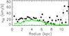 |
Fig. 12 Amplitude v02 of the combined k = 0 and k = 2 harmonics of the Hα velocity field of M 99 (filled symbols). The dotted lines indicate the result for the model velocity field of the centered-Einasto halo with vR, while the dashed and solid lines indicate models of the shifted-Einasto halo with and without vR, respectively. |
In this section, we thus explore the possibility that the gravitational potential of total matter is additionally lopsided under the influence of a spherical dark matter halo whose center is shifted with respect to the center of luminous baryons. For this purpose, we added two parameters to the modeling, which correspond to offsets δx and δy of the dark matter center to the coordinates x−y of the center of luminous matter, respectively. The resolved velocity map of dark matter is estimated in a new grid of coordinates centered on (δx,δy), and added quadratically to that of luminous baryons, where the latter remains the same as in previous sections, i.e. centered on x = y = 0. For simplicity, we assume that the gravity center of dark matter remains in the disk midplane. Such least-squares fittings are referred to as shifted-halo models in Tables D.1 and D.2 (Appendix D). As a result, we find similarities with the centered-halo modeling: The Einasto model remains the model that is the most appropriate, the asymmetric case provides better results than the axisymmetric case, and the modeling with vR provide better fittings than those without these motions. However, there are numerous differences between these models and the centered-halo configuration. First, the AIC tests show that all models with shifted dark matter haloes are more likely than with centered dark matter haloes, and the formal errors on the halo parameters are significantly smaller. Second, the center of the dark halo is found no more coincident with the luminous center. A mean total shift of 2.5 ± 0.2 kpc (2.2 ± 0.3 kpc) is implied by the asymmetric modeling with noncircular motions (without, respectively). The consideration of noncircular velocities thus tends to increase the DM shift. Compared to the axisymmetric modeling, the nonuniformity of circular motions also tends to increase the offset, but only at a level of 0.1 kpc. A shift of 2.2−2.5 kpc is significant as it corresponds to more than 15 times the angular sampling of the stellar density and Fabry-Perot interferometry maps. Third, the resulting haloes have become core dominated. The Einasto density profile is now considerably shallower in its center (slopes at R = 0.27 kpc of −0.01 and −0.02 (± 0.01) with and without radial motions, respectively), and the pseudoisothermal sphere has become more likely than the NFW cusp. Moreover, the concentration of dark matter is significantly smaller than in the centered-halo case. Figure 13 shows the modeled velocity and residual velocity maps for the shifted Einasto halo with the vR component. We estimate that on average, the beneficial impact of the shifted-halo occurs beyond R ~ 3 kpc. Inside that radius, the scatter of residuals is roughly equivalent, and sometimes larger than in the centered-halo case, depending on the considered halo shape and the contribution from vR. The shifted-halo model correctly reproduces most of the v02 amplitude (solid and dashed lines in Fig. 12), implying that the assumption that the total potential is lopsided is valid.
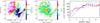 |
Fig. 13 Left: modeled velocity field of M 99 from the 2D asymmetric case for the shifted Einasto halo with vR motions. Contours are the same as in Fig. 11. Middle: corresponding residual velocity field. Right: comparison of major axis l.o.s. velocities of the observation with the centered-halo and shifted-halo cases. Blue and red symbols indicate the approaching and receding sides, respectively. Open dotted and crossed symbols indicate the observed velocity field, filled diamonds, and triangles for the asymmetric centered- and shifted-Einasto models, respectively, with the contribution from vR. |
However, a lag with respect to the observed v02 still exists in the innermost regions. In addition, as in the centered-halo configuration, differences from the observation are not only evident in the center and along the minor axis of the residual maps, but they are also observed along the major axis of the velocity fields. Figure 13 (right panel) indeed shows that none of our asymmetric models succeeds in correctly reproducing the difference between the approaching and receding disk halves at small radii, whether the dark matter component is aligned with the luminous baryons or not. More importantly, only the receding motions are fairly well reproduced and the approaching motions for the centered or shifted halo models remain quite similar to the receding motions. Though promising, the shifted-halo solution also turns out to be incomplete to explain the inner lopsidedness of M 99. It appears here that an additional dynamical process causing more asymmetric motions than our predictions is required at small radius. What could explain this discrepancy? If it comes from the incorrect assumption that circularity dominates, then one should question the relevance of performing mass models of galaxies harboring lopsided kinematics and structure. At the same time, nonuniform vR motions that would dominate the nonuniform vθ at these radii cannot explain the discrepancy because vR does not project along the major axis, whereas the inner lopsided effect is obvious along this axis. We then reject the possibility of perturbed motions by a central bar because the stellar potential rules out its presence, and the kinematical signature of a bar should be bisymmetric. A possible origin could be that vertical motions are finally not as negligible as initially thought. It was shown that the l.o.s. width of the Hα profiles is slightly larger toward the center. Larger dispersions may be partly explained by the observed larger nonuniformity of circular motions. It may be also due to a larger scatter of vertical motions, if the ellispoid of velocity dispersion is isotropic. The impact of fixing vz = 0 instead of truly varying vertical motions with radius is to generate artificial variations of vsys or, more precisely, of the k = 0 Fourier coefficient (Appendix B). The reason for this bias is that the vz projection along the l.o.s. does not depend on θ but simply adds linearly to the systemic velocity (Eq. (1)). Though vz ≠ 0 could explain some of the observed variation of the k = 0 term in the velocity field (Fig. A.4), a vz-induced mechanism cannot impact the k = 2 coefficients, however.
We are left with the hypothesis that our modeling could be improved by the action of circular motions with larger nonuniformity than predicted, particularly for the approaching side of the galaxy because it is the most discrepant disk region with respect to the expectations. We reject the possibility that the SPS models yielded incorrect stellar masses and velocities for this disk half because they have been performed following a homogeneous approach all through the field of view. Instead, we think that a mechanism where the velocity contribution from dark matter is nonuniform is more worthwhile to consider. It does not seem unrealistic that the gravitational potential of dark matter is lopsided as well, owing to the perturbed nature of both the stellar and gaseous components in M 99. In this case, our scenario of shifted DM component with respect to the luminous disk is anecdotal, as it would be only a signature of a more complex lopsided distribution of dark matter. Further modeling of the velocity field of M 99 is needed to constrain this possibly more asymmetric density and velocity distribution of dark matter.
Off-centered density peak and lopsided distribution of dark matter haloes have been evidenced in cosmological hydrodynamics simulations (Kuhlen et al. 2013; Schaller et al. 2015). The typical distance between the simulated dark matter density peak to the stellar density peak, or to the position of the minimum of the total gravitational potential, is ∝ 100 pc. Interestingly, the presence of a peak offset for the simulated halo of Kuhlen et al. (2013) is tightly linked to the core-dominated nature of its density profile. The significantly larger shift found for M 99 appears to conflict with the collisional simulations, but the concomitance of the inner density flatness with the halo shift in M 99 is an observational support to the simulations. A dynamical mechanism that motivates a disturbed DM halo, and maybe a misalignment with luminous matter, could be a tidal event (Jog & Combes 2009; van Eymeren et al. 2011). A tidal interaction between M 99 and a massive companion has actually occurred in the past Gyr, maybe 750 Myr ago (Duc & Bournaud 2008). The interaction with the gravitational field of the Virgo cluster is likely very active too, as M 99 has entered the cluster (Vollmer et al. 2005). If triggered by such tidal processes, the DM core shift seems to be a long-lived dynamical event in M 99. However, a tidal scenario only seems problematic to explain the amplitude of the v02 asymmetry in the innermost regions. Such a scenario is expected to enhance the strength of lopsidedness with radius (e.g., Jog & Combes 2009), while a roughly constant kinematical asymmetry is measured within R ~ 7 kpc. A mechanism other than a tidal event thus remains to be proposed for the origin of the innermost lopsidedness of the total mass distribution of M 99, including that of the dark matter component.
7. Conclusions
We have presented a new methodology to model the mass distribution of disk galaxies directly from bidimensional observables, resolved stellar population synthesis models, high-sensitivity gas density maps, and high-resolution velocity fields. The methodology makes use of hyperpotentials to derive the 3D gravitational potentials of luminous matter and the relevant azimuthal and radial forces without the intervention of a softening length. The 3D strategy is advantageous to estimate the circular motions through nonaxisymmetric features like spiral arms since the 2D distribution of circular velocity in disk midplanes naturally stems from asymmetric potentials.
Applied to multiwavelength observations of the late-type spiral galaxy Messier 99, the method led us to the following results:
-
The gravitational potential of the disks of stars, atomic, and molecular gas is perturbed by dominant m = 1 and m = 2 modes corresponding to lopsidedness and grand-design spiral arms. The importance of the perturbations decreases with the mass surface density. Amplitudes of perturbations in the stellar disk thus represent no more than 4% of that of the axisymmetric mode, while they can be as high as 16% for the atomic gas component.
-
On a global scale, the radial force strongly dominates the tangential force, implying that M 99 may be perceived as totally dominated by uniform circular rotation.
-
On local scales however, the radial forces are comparable to the tangential forces, implying that the circular motions are highly nonuniform. Nonuniformity of circular velocities turns out to be the rule, while uniformity, i.e. axisymmetry, is the exception. The inner disk regions are those where nonuniformity is larger. The strongest variations occur through spiral arms. Gas self-gravity is not negligible in the densest parts of spiral arms as it can account for, on average, up to 50% of the nonuniformity.
-
It makes it possible to fit 2D, asymmetric mass distribution models to the velocity field of the galaxy. The modeled velocity fields harbors wiggles along the spiral arms, as a direct consequence of nonuniform circular motions. The number of degrees of freedom has become considerably larger than for the rotation curve decomposition, yielding more constrained fittings and parameters for the dark matter halo. Compared to an axisymmetric viewpoint, the use of asymmetric velocities improves the mass modeling, as the scatter and amplitude of residual velocities have decreased. Dealing with asymmetric circular velocities in M 99 makes the density profile of the dark matter component less cuspy than in the axisymmetric case. This effect is more prominent for a dark matter model whose inner density slope is allowed to vary, such as the Einasto halo, than for models with constant inner slope, such as the NFW cusp or the pseudoisothermal sphere.
-
The 2D strategy also makes it possible to take into account (uniform) noncircular motions vR in the mass modeling. Noncircular motions also make the DM density profile less cuspy in M 99, but to a lower degree than for the nonuniform circular motions.
-
On the one hand, the 2D asymmetric fittings prefer cuspy Einasto or NFW haloes to the pseudoisothermal sphere in a traditional case where the dark matter halo is centered on the luminous mass component. On the other hand, a more likely model introducing a dark matter halo shifted from the luminous center requires a core dark matter halo. That shifted-halo modeling succeeds in reproducing a large part of the observed kinematical lopsidedness, contrary to the centered-halo modeling. However, none of these models can reproduce the lopsidedness in the innermost regions of M 99. All these results likely reflect the need for an asymmetric (lopsided) dark matter distribution in M 99. This would not be surprising owing to the lopsided nature of disks of stars and gas. Tidal effects from a companion and/or the Virgo cluster tidal field could partly explain the lopsidedness. However, another process to be identified is needed to explain the innermost lopsidedness of the total mass distribution and of the dark matter halo of M 99.
The new strategy is very promising for galactic dynamics. We envisage testing the reproducibility of such results on a larger sample of galaxies of various morphologies and masses. Future papers from this series will focus on other massive late-type spirals, as well as lower surface density, dark-matter dominated disks, which are at the origin of the cusp-core controversy. Velocity fields of these types of galaxies are rich with information that are worth investigating. Furthermore, as resolved SPS models as in Zibetti et al. (2009), Corbelli et al. (2014), Meidt et al. (2014), and Rahmani et al. (2016) are in their early stages, derivations of many more stellar density maps is strongly encouraged to be able to quantify the asymmetries of the gravitational potential of stellar disks directly. This is more straightforward for the gas component since atomic and molecular surface density maps are routinely acquired with mm and cm arrays. Finally, we hope that this research will have a broader impact because the concepts developed here can be easily transferable to the Milky Way and other types of disks, from protostellar disks to high-redshift galaxies.
Acknowledgments
Laurent Chemin acknowledges the financial support from CNES. We are grateful to an anonymous referee whose suggestions led to clarify the discussion, content, and structure of the manuscript. This research has made use of the NASA/IPAC Extragalactic Database (NED), which is operated by the Jet Propulsion Laboratory, California Institute of Technology, under contract with the National Aeronautics and Space Administration (http://ned.ipac.caltech.edu). We acknowledge the usage of the HyperLeda database (leda.univ-lyon1.fr). The SDSS image is from cosmo.nyu.edu/hogg/rc3, prepared by David W. Hogg, Michael R. Blanton, and the Sloan Digital Sky Survey Collaboration.
References
- Akaike, H. 1974, IEEE Transactions on Automatic Control, 19, 716 [Google Scholar]
- Angiras, R. A., Jog, C. J., Omar, A., & Dwarakanath, K. S. 2006, MNRAS, 369, 1849 [NASA ADS] [CrossRef] [Google Scholar]
- Angiras, R. A., Jog, C. J., Dwarakanath, K. S., & Verheijen, M. A. W. 2007, MNRAS, 378, 276 [NASA ADS] [CrossRef] [Google Scholar]
- Athanassoula, E. 1992, MNRAS, 259, 345 [NASA ADS] [CrossRef] [Google Scholar]
- Barnes, D. J., Kawata, D., & Wu, K. 2012, MNRAS, 420, 3195 [NASA ADS] [CrossRef] [Google Scholar]
- Bershady, M. A., Martinsson, T. P. K., Verheijen, M. A. W., et al. 2011, ApJ, 739, L47 [NASA ADS] [CrossRef] [Google Scholar]
- Binney, J., & Tremaine, S. 2008, Galactic Dynamics: Second Edition (Princeton University Press) [Google Scholar]
- Bournaud, F., Combes, F., Jog, C. J., & Puerari, I. 2005, A&A, 438, 507 [NASA ADS] [CrossRef] [EDP Sciences] [Google Scholar]
- Bruzual, G., & Charlot, S. 2003, MNRAS, 344, 1000 [NASA ADS] [CrossRef] [Google Scholar]
- Buta, R. J., & Zhang, X. 2009, ApJS, 182, 559 [NASA ADS] [CrossRef] [Google Scholar]
- Cardone, V. F., Piedipalumbo, E., & Tortora, C. 2005, MNRAS, 358, 1325 [NASA ADS] [CrossRef] [Google Scholar]
- Charlot, S., & Fall, S. M. 2000, ApJ, 539, 718 [NASA ADS] [CrossRef] [Google Scholar]
- Chemin, L., Cayatte, V., Balkowski, C., et al. 2005a, A&A, 436, 469 [NASA ADS] [CrossRef] [EDP Sciences] [Google Scholar]
- Chemin, L., Hernandez, O., Balkowski, C., Carignan, C., & Amram, P. 2005b, ArXiv Astrophysics e-prints [arXiv:astro-ph/0512514] [Google Scholar]
- Chemin, L., Balkowski, C., Cayatte, V., et al. 2006, MNRAS, 366, 812 [NASA ADS] [CrossRef] [Google Scholar]
- Chemin, L., de Blok, W. J. G., & Mamon, G. A. 2011, AJ, 142, 109 [NASA ADS] [CrossRef] [Google Scholar]
- Chemin, L., Renaud, F., & Soubiran, C. 2015, A&A, 578, A14 [NASA ADS] [CrossRef] [EDP Sciences] [Google Scholar]
- Chung, A., van Gorkom, J. H., Kenney, J. D. P., Crowl, H., & Vollmer, B. 2009, AJ, 138, 1741 [NASA ADS] [CrossRef] [Google Scholar]
- Combes, F., & Sanders, R. H. 1981, A&A, 96, 164 [NASA ADS] [Google Scholar]
- Corbelli, E., Thilker, D., Zibetti, S., Giovanardi, C., & Salucci, P. 2014, A&A, 572, A23 [NASA ADS] [CrossRef] [EDP Sciences] [Google Scholar]
- da Cunha, E., Charlot, S., & Elbaz, D. 2008, MNRAS, 388, 1595 [NASA ADS] [CrossRef] [Google Scholar]
- Daigle, O., Carignan, C., Hernandez, O., Chemin, L., & Amram, P. 2006, MNRAS, 368, 1016 [NASA ADS] [CrossRef] [Google Scholar]
- Dalcanton, J. J., & Stilp, A. M. 2010, ApJ, 721, 547 [NASA ADS] [CrossRef] [Google Scholar]
- de Blok, W. J. G. 2010, Adv. Astron., 2010, 5 [Google Scholar]
- de Blok, W. J. G., & Bosma, A. 2002, A&A, 385, 816 [NASA ADS] [CrossRef] [EDP Sciences] [Google Scholar]
- de Blok, W. J. G., Walter, F., Brinks, E., et al. 2008, AJ, 136, 2648 [NASA ADS] [CrossRef] [Google Scholar]
- Dicaire, I., Carignan, C., Amram, P., et al. 2008, MNRAS, 385, 553 [NASA ADS] [CrossRef] [Google Scholar]
- Duc, P.-A., & Bournaud, F. 2008, ApJ, 673, 787 [NASA ADS] [CrossRef] [Google Scholar]
- Epinat, B., Amram, P., & Marcelin, M. 2008a, MNRAS, 390, 466 [NASA ADS] [Google Scholar]
- Epinat, B., Amram, P., Marcelin, M., et al. 2008b, MNRAS, 388, 500 [NASA ADS] [CrossRef] [Google Scholar]
- Epinat, B., Amram, P., Balkowski, C., & Marcelin, M. 2010, MNRAS, 401, 2113 [NASA ADS] [CrossRef] [Google Scholar]
- Franx, M., van Gorkom, J. H., & de Zeeuw, T. 1994, ApJ, 436, 642 [NASA ADS] [CrossRef] [Google Scholar]
- Freedman, W. L., Madore, B. F., Mould, J. R., et al. 1994, Nature, 371, 757 [NASA ADS] [CrossRef] [Google Scholar]
- Gentile, G., Burkert, A., Salucci, P., Klein, U., & Walter, F. 2005, ApJ, 634, L145 [NASA ADS] [CrossRef] [Google Scholar]
- Gentile, G., Salucci, P., Klein, U., & Granato, G. L. 2007, MNRAS, 375, 199 [NASA ADS] [CrossRef] [Google Scholar]
- Governato, F., Brook, C., Mayer, L., et al. 2010, Nature, 463, 203 [NASA ADS] [CrossRef] [PubMed] [Google Scholar]
- Grand, R. J. J., Kawata, D., & Cropper, M. 2012, MNRAS, 426, 167 [NASA ADS] [CrossRef] [Google Scholar]
- Hayashi, E., & Navarro, J. F. 2006, MNRAS, 373, 1117 [NASA ADS] [CrossRef] [Google Scholar]
- Huré, J.-M. 2013, A&A, 554, A45 [NASA ADS] [CrossRef] [EDP Sciences] [Google Scholar]
- Jog, C. J. 1997, ApJ, 488, 642 [NASA ADS] [CrossRef] [Google Scholar]
- Jog, C. J. 2000, ApJ, 542, 216 [NASA ADS] [CrossRef] [Google Scholar]
- Jog, C. J. 2002, A&A, 391, 471 [NASA ADS] [CrossRef] [EDP Sciences] [Google Scholar]
- Jog, C. J., & Combes, F. 2009, Phys. Rep., 471, 75 [NASA ADS] [CrossRef] [Google Scholar]
- Kam, Z. S., Carignan, C., Chemin, L., Amram, P., & Epinat, B. 2015, MNRAS, 449, 4048 [NASA ADS] [CrossRef] [Google Scholar]
- Kamphuis, J., & Briggs, F. 1992, A&A, 253, 335 [NASA ADS] [Google Scholar]
- Kawata, D., Thom, C., & Gibson, B. K. 2003, PASA, 20, 263 [NASA ADS] [CrossRef] [Google Scholar]
- Kawata, D., Okamoto, T., Gibson, B. K., Barnes, D. J., & Cen, R. 2013, MNRAS, 428, 1968 [NASA ADS] [CrossRef] [Google Scholar]
- Kawata, D., Gibson, B. K., Barnes, D. J., Grand, R. J. J., & Rahimi, A. 2014a, MNRAS, 438, 1208 [NASA ADS] [CrossRef] [Google Scholar]
- Kawata, D., Hunt, J. A. S., Grand, R. J. J., Pasetto, S., & Cropper, M. 2014b, MNRAS, 443, 2757 [NASA ADS] [CrossRef] [Google Scholar]
- Kranz, T., Slyz, A., & Rix, H.-W. 2001, ApJ, 562, 164 [NASA ADS] [CrossRef] [Google Scholar]
- Kriek, M., Labbé, I., Conroy, C., et al. 2010, ApJ, 722, L64 [NASA ADS] [CrossRef] [Google Scholar]
- Kuhlen, M., Guedes, J., Pillepich, A., Madau, P., & Mayer, L. 2013, ApJ, 765, 10 [NASA ADS] [CrossRef] [Google Scholar]
- Leroy, A. K., Walter, F., Bigiel, F., et al. 2009, AJ, 137, 4670 [NASA ADS] [CrossRef] [Google Scholar]
- Maciejewski, W. 2004, MNRAS, 354, 892 [NASA ADS] [CrossRef] [Google Scholar]
- Makarov, D., Prugniel, P., Terekhova, N., Courtois, H., & Vauglin, I. 2014, A&A, 570, A13 [Google Scholar]
- Mamon, G. A., & Łokas, E. L. 2005, MNRAS, 363, 705 [NASA ADS] [CrossRef] [Google Scholar]
- Maraston, C. 2005, MNRAS, 362, 799 [NASA ADS] [CrossRef] [Google Scholar]
- Martinsson, T. P. K., Verheijen, M. A. W., Westfall, K. B., et al. 2013, A&A, 557, A131 [NASA ADS] [CrossRef] [EDP Sciences] [Google Scholar]
- Meidt, S. E., Schinnerer, E., van de Ven, G., et al. 2014, ApJ, 788, 144 [NASA ADS] [CrossRef] [Google Scholar]
- Melnick, J., & De Propris, R. 2014, A&A, 572, A5 [NASA ADS] [CrossRef] [EDP Sciences] [Google Scholar]
- Minchev, I., Famaey, B., Quillen, A. C., et al. 2012, A&A, 548, A127 [NASA ADS] [CrossRef] [EDP Sciences] [Google Scholar]
- Minchin, R., Davies, J., Disney, M., et al. 2007, ApJ, 670, 1056 [NASA ADS] [CrossRef] [Google Scholar]
- Navarro, J. F., Frenk, C. S., & White, S. D. M. 1997, ApJ, 490, 493 [NASA ADS] [CrossRef] [Google Scholar]
- Navarro, J. F., Hayashi, E., Power, C., et al. 2004, MNRAS, 349, 1039 [NASA ADS] [CrossRef] [Google Scholar]
- Oh, S.-H., de Blok, W. J. G., Walter, F., Brinks, E., & Kennicutt, Jr., R. C. 2008, AJ, 136, 2761 [NASA ADS] [CrossRef] [Google Scholar]
- Phookun, B., Vogel, S. N., & Mundy, L. G. 1993, ApJ, 418, 113 [NASA ADS] [CrossRef] [Google Scholar]
- Planck Collaboration XIII. 2015, A&A, submitted [arXiv:1502.01589] [Google Scholar]
- Quillen, A. C., Dougherty, J., Bagley, M. B., Minchev, I., & Comparetta, J. 2011, MNRAS, 417, 762 [NASA ADS] [CrossRef] [Google Scholar]
- Rahman, N., Bolatto, A. D., Wong, T., et al. 2011, ApJ, 730, 72 [NASA ADS] [CrossRef] [Google Scholar]
- Rahmani, S., Lianou, S., & Barmby, P. 2016, MNRAS, 456, 4128 [NASA ADS] [CrossRef] [Google Scholar]
- Randriamampandry, T. H., Combes, F., Carignan, C., & Deg, N. 2015, MNRAS, 454, 3743 [NASA ADS] [CrossRef] [Google Scholar]
- Renaud, F., Bournaud, F., Emsellem, E., et al. 2013, MNRAS, 436, 1836 [NASA ADS] [CrossRef] [Google Scholar]
- Renaud, F., Bournaud, F., Emsellem, E., et al. 2015, MNRAS, 454, 3299 [NASA ADS] [CrossRef] [Google Scholar]
- Retana-Montenegro, E., van Hese, E., Gentile, G., Baes, M., & Frutos-Alfaro, F. 2012, A&A, 540, A70 [NASA ADS] [CrossRef] [EDP Sciences] [Google Scholar]
- Rix, H.-W., & Zaritsky, D. 1995, ApJ, 447, 82 [NASA ADS] [CrossRef] [Google Scholar]
- Sackett, P. D. 1997, ApJ, 483, 103 [NASA ADS] [CrossRef] [Google Scholar]
- Schaller, M., Robertson, A., Massey, R., Bower, R. G., & Eke, V. R. 2015, MNRAS, 453, L58 [NASA ADS] [CrossRef] [Google Scholar]
- Schoenmakers, R. H. M. 1999, Ph.D Thesis, University of Groningen [Google Scholar]
- Schoenmakers, R. H. M., Franx, M., & de Zeeuw, P. T. 1997, MNRAS, 292, 349 [NASA ADS] [CrossRef] [Google Scholar]
- Sellwood, J. A., & Binney, J. J. 2002, MNRAS, 336, 785 [NASA ADS] [CrossRef] [Google Scholar]
- Simon, J. D., Bolatto, A. D., Leroy, A., Blitz, L., & Gates, E. L. 2005, ApJ, 621, 757 [NASA ADS] [CrossRef] [Google Scholar]
- Spekkens, K., & Sellwood, J. A. 2007, ApJ, 664, 204 [NASA ADS] [CrossRef] [Google Scholar]
- Swaters, R. A., Schoenmakers, R. H. M., Sancisi, R., & van Albada, T. S. 1999, MNRAS, 304, 330 [NASA ADS] [CrossRef] [Google Scholar]
- Swaters, R. A., Sancisi, R., van Albada, T. S., & van der Hulst, J. M. 2009, A&A, 493, 871 [NASA ADS] [CrossRef] [EDP Sciences] [Google Scholar]
- Valenzuela, O., Rhee, G., Klypin, A., et al. 2007, ApJ, 657, 773 [NASA ADS] [CrossRef] [Google Scholar]
- van der Kruit, P. C., & Searle, L. 1981, A&A, 95, 105 [NASA ADS] [Google Scholar]
- van Eymeren, J., Jütte, E., Jog, C. J., Stein, Y., & Dettmar, R.-J. 2011, A&A, 530, A29 [NASA ADS] [CrossRef] [EDP Sciences] [Google Scholar]
- Vollmer, B., Huchtmeier, W., & van Driel, W. 2005, A&A, 439, 921 [NASA ADS] [CrossRef] [EDP Sciences] [Google Scholar]
- Wada, K. 1994, PASJ, 46, 165 [NASA ADS] [Google Scholar]
- Walter, F., Brinks, E., de Blok, W. J. G., et al. 2008, AJ, 136, 2563 [NASA ADS] [CrossRef] [Google Scholar]
- Westfall, K. B., Bershady, M. A., Verheijen, M. A. W., et al. 2011, ApJ, 742, 18 [NASA ADS] [CrossRef] [Google Scholar]
- Wong, T., Blitz, L., & Bosma, A. 2004, ApJ, 605, 183 [NASA ADS] [CrossRef] [Google Scholar]
- Yoachim, P., & Dalcanton, J. J. 2006, AJ, 131, 226 [NASA ADS] [CrossRef] [Google Scholar]
- Zaritsky, D., & Rix, H.-W. 1997, ApJ, 477, 118 [NASA ADS] [CrossRef] [Google Scholar]
- Zhang, X., & Buta, R. J. 2007, AJ, 133, 2584 [NASA ADS] [CrossRef] [Google Scholar]
- Zibetti, S. 2009, ArXiv e-prints [arXiv:0911.4956] [Google Scholar]
- Zibetti, S., Charlot, S., & Rix, H.-W. 2009, MNRAS, 400, 1181 [NASA ADS] [CrossRef] [Google Scholar]
- Zibetti, S., Gallazzi, A., Charlot, S., Pierini, D., & Pasquali, A. 2013, MNRAS, 428, 1479 [NASA ADS] [CrossRef] [Google Scholar]
Appendix A: Harmonics of the gravitational potentials of luminous matter
This Appendix presents the axisymmetric potential of the bulge, and the analysis of the harmonic decomposition of the individual gravitational potentials for the asymmetric stellar and gaseous disks of M 99.
For each mass component but the bulge, the gravitational potential in the z = 0 kpc midplane, Φ(R,θ,z = 0) (abridged in Φ(R,θ)), is given by 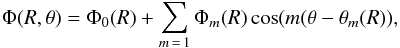 (A.1)where Φ0 is the amplitude of the axisymmetric component, and Φm(R) and θm(R) are the amplitudes and phases of the mth harmonics. Orders up to m = 3 are enough for both stellar and gaseous disks. The results for Φm(R) and θm(R) are presented in Figs. A.1 and A.2.
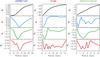 |
Fig. A.1 Amplitude Φm of the harmonics of gravitational potential for the stellar and gaseous disks of M 99, in units of 103 km2 s-2, with m = 0,1,2,3. The left-hand column is for the atomic gas disk, the middle one for the stellar disk and the right-hand column for the molecular gas disk. For the stellar component, the axisymmetric potential of the bulge has been removed. |
For the stellar disk, the m = 1 and m = 2 perturbations are stronger in the center. The m = 1 amplitude dominates the m = 2 value inside R = 4 kpc, reaching 5% of the unperturbed m = 0 mode at R ~ 0.7 kpc. The m = 2 perturbation is slightly stronger than m = 1 at R> 4 kpc. It reaches ~ 3% of the unperturbed mode at R = 1 kpc and ~ 4% at R = 9.5 kpc. As these two modes lie at similar radii, it implies that the central m = 2 spiral is strongly lopsided or, alternatively, that a prominent m = 1 spiral coexists with the m = 2 spiral structure, but at different phase angle. The m = 3 amplitude is more scattered than the others, never exceeding 3% that of the unperturbed mode.
For the disk of molecular gas, it is the m = 2 spiral pattern that dominates the perturbations in majority with an amplitude reaching ~9% of the molecular m = 0 coefficient at R = 2 kpc. We point out the smooth variation of the phase angle of the m = 2 pattern as a function of radius. The m = 1 amplitudeis slightly stronger than the m = 2 mode at R = 0.5 and 4 kpc. The m = 2 spiral structure is thus lopsided inside R = 0.5 kpc, or accompanied by a dephased single molecular arm. Here again, the m = 3 amplitude is more scattered and never exceeds 3% of the m = 0 amplitude within R = 6 kpc.
For the atomic gas disk, the m = 2 perturbation admits a minimum amplitude at R ~ 10 kpc, for a relatively constant phase angle within R = 5−15 kpc. That m = 2 mode coincides well with the spiral structure of the stellar distribution. The maximum amplitudes of the m = 2 mode reach ~ 10% that of the m = 0 mode. The amplitude of the m = 1 mode is a minimum at R ~ 12 kpc and reaches more than 20% that of the m = 0 amplitude beyond that radius. Since the m = 1 spiral is an extension of one of the two spiral arms (Fig. 4), it explains the offset of about 2 kpc between the dips of the m = 1 and m = 2 potentials. Furthermore, since the m = 1 mode dominates all other perturbations, it is likely that the outer one-arm perturbation is at the origin of the m = 2 spiral structure of M 99, and not the opposite. As for the m = 3 mode, it is weaker and shows two major patterns at 7 and 13 kpc, which are dephased by ~ π/ 3 from each other. Whether this mode is an actual organized m = 3 spiral structure is a matter of debate. More simply, it likely reflects the complexity of the distribution and gravitational potential of the atomic gas beyond the stellar disk. For R> 20 kpc, the m = 2 and m = 3 modes also present features of very weak amplitude, but which are evident in the phase angle profiles. This outer m = 2 feature could be a genuine spiral structure. It could also be the signature of a Hi warp of the atomic gas disk, even if Hi densities have been deprojected under a constant inclination angle (Sect. 3.2). Gas accretion on the Hi disk outskirts after a tidal interaction with a companion, as suggested by numerical simulations of Vollmer et al. (2005) and Duc & Bournaud (2008), is likely to generate a disk warping. If it exists, this Hi warp cannot be bisymmetric because of the more prominent m = 1 pattern. This explains the difficulty we faced when fitting an axisymmetric tilted-ring model of the Hi velocity field at these radii.
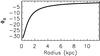 |
Fig. A.3 Gravitational potential of the spherical stellar bulge of M 99, in units of 103 km2 s-2. |
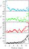 |
Fig. A.4 Amplitude vk of the kinematical Fourier mode k for the observed velocity field of M 99 in units of km s-1. |
Appendix B: Harmonics of the Hα velocity field
This Appendix presents the results of the Fourier analysis of the Hα velocity field of M 99. At a given radius, the impact of kinematical asymmetries induced by perturbations, such as spiral arms, bars, lopsidedness, and warp, makes the velocity fluctuate around the axisymmetric component (Franx et al. 1994; Schoenmakers et al. 1997; Binney & Tremaine 2008). The variations of vθ and vR are linked to the axisymmetric vc and the amplitudes, phases, and pattern speeds of the gravitational potentials of the dynamical perturbations. Schoenmakers et al. (1997) showed it is possible to estimate the kinematical variations from a harmonic decomposition of velocity fields.
We thus expand the standard model of Eq. (1) into 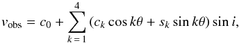 (B.1)where ck and sk are the Fourier velocity coefficients of harmonic order k (k is an integer). The c0 coefficient is equivalent to the systemic velocity vsys of Eq. (1). Unless constrained by direct methods, the additional vertical component vz must not be used here because its projection on the l.o.s. is degenerated with variations of the systemic velocity.
Schoenmakers et al. (1997) also showed that a perturbation of the potential of order m induces kinematical components of order k = m−1 and k = m + 1. Therefore, as the m = 3 order is the weakest perturbing mode detected in the gravitational potentials of luminous matter, kinematical harmonics up to k = 4 can be derived. We thus fitted Eq. (B.1) to the Hα data up to k = 4 with obligatory uniform weightings, and fixed i, Γ, and the coordinates of the kinematical center to the abovementioned values. The width of the radial bins is adaptive and chosen to have more than 60 d.o.fs per ring for accurate fittings. We derived the kinematical amplitudes vk of the harmonics by  for k> 1, and
  . No k = 1 amplitude is derived because the s1 and c1 coefficients are very similar to vR and vθ from Eq. (1) and Fig. 3. This means that the decomposition is mostly efficient in modeling residual velocities resulting from subtracting axisymmetric models to an observed velocity map, like the map shown in Figs. 11 and 13.
Figure A.4 shows the resulting profiles of the Fourier amplitudes. The phases are not shown as they do not present any particular interest for the analysis. The amplitude becomes smaller for larger kinematical modes for R< 7 kpc. Beyond that radius, the amplitude and the scatter increase and are larger for larger orders. Those variations at larger radii can be seen as direct responses to the increasing strength of perturbations of the stellar and neutral gas disk potentials relative to the axisymmetric potentials (Fig. 7) and, likely , of dark matter as well. The number of d.o.fs per radial bin decreases from R ~ 4 kpc, which explains the larger scatter of velocities at large radius. However, a smaller number of d.o.fs cannot be at the origin of the increase of the kinematical asymmetries. For instance, the number of d.o.fs at R ~ 2 kpc is similar to that at R ~ 10.5 kpc, while the asymmetries at R ~ 2 kpc are much smaller. The variation of v0, principally in the center, does not mean that the systemic velocity varies with radius, but the impact of the galaxy lopsidedness, and maybe of non-negligible vertical velocities. The signature of the m = 1 perturbation is confirmed by the detection of a v2 ~ 20 km s-1 component out to R = 7 kpc. That v2 component is very likely dominated by the effects of the m = 1 pertubation, and not as much by the weakest m = 3 perturbations. A confirmation of the small impact of the m = 3 mode is the smaller component v4 ~ 5 km s-1 than v2 for R< 7 kpc. As for the v3 component, it shows wiggles caused by m = 2 perturbing modes, among which are those identified in the molecular gas and stellar disk potentials. Effects of the m = 2 perturbations were already observed in the k = 1 order as departures of the 1D axisymmetric mass model from the rotation curve (Fig. 3). The kinematical asymmetries of M 99 are larger than those generally found in other dwarf and massive disks (Schoenmakers et al. 1997; Schoenmakers 1999; Gentile et al. 2007; Oh et al. 2008). This discrepancy is explained by the lower angular resolution of their Hi velocity fields used to perform the harmonic analysis. Large synthesized beams in radio interferometry indeed dilute the kinematics and lower the impact of asymmetries in the kinematical and dynamical modeling. Similar amplitudes to those of M 99 were found in other galaxies for k = 2 components from Hα observations (e.g., Chemin et al. 2006; Spekkens & Sellwood 2007), which confirms that high-resolution data are more appropriate to estimate accurate amplitudes of kinematical asymmetries.
Appendix C: Rotation curve, radial velocity, and velocity dispersion
M 99 rotation curve, radial velocity, and velocity dispersion.
Appendix D: Results of the mass distribution models
Results of the mass distribution modeling of the rotation curve (1D) and velocity field (2D) of M 99.
Comparisons between the various mass models: halo vs. halo, axisymmetric vs. asymmetric cases, with vs. without the vR component, and centered- vs. shifted-halo.
All Tables
Results of the mass distribution modeling of the rotation curve (1D) and velocity field (2D) of M 99.
Comparisons between the various mass models: halo vs. halo, axisymmetric vs. asymmetric cases, with vs. without the vR component, and centered- vs. shifted-halo.
All Figures
|
Fig. 1 Composite SDSS gri-image of the grand-design spiral galaxy M 99. North is up; east is left. The image size is 7′ × 6.3′. |
| In the text | |
|
Fig. 2 Hα integrated emission, velocity field, and velocity dispersion map of M 99 (from left to right, respectively). |
| In the text | |
|
Fig. 3 Left and middle: profiles of tangential and radial velocity of M 99. Shaded area indicates the 1σ rms from the fittings. A green solid line represents the fitting for the whole disk, while blue dotted and red crossed circles are respectively the results for the approaching and receding sides fitted separately. Right panel: Hα velocity dispersion of M 99. Symbols represent the observed dispersion; the dashed line is a smooth model of the observation used to derive the asymmetric drift. |
| In the text | |
|
Fig. 4 Surface density maps for the atomic gas, stellar and molecular gas disks of M 99 (from left to right, respectively). Densities (in M⊙ pc-2) are shown in a decimal logarithmic scale. |
| In the text | |
|
Fig. 5 Left: mass surface density profile of stars in M 99. A bulge-disk decomposition model (green solid line) to the observed profile (symbols) is seen, as well as bulge and disk components (red dashed lines). Right: axisymmetric mass distribution model of M 99. The rotation curve is represented with filled symbols, and its model with an orange solid line. Contributions from the stellar bulge and disk are shown with red dashed lines, from the atomic and molecular gas disks with blue dash-dotted lines, and from the dark matter component with green open symbols. The dark matter model is the best-fit NFW halo whose parameters are given in Table D.1. |
| In the text | |
|
Fig. 6 Gravitational potential (Φ), tangential, and radial acceleration (gθ and gR, respectively) maps of the disks of the atomic, molecular gas, and stellar components of M 99. These maps are for the z = 0 kpc midplane. The axisymmetric contribution from the bulge potential is not included in the stellar disk component. |
| In the text | |
|
Fig. 7 Fraction (in %) of the perturbed potential to the unperturbed potential for luminous matter in M 99. The red solid (dotted) line is for the stellar disk (stellar bulge+disk) potential, green dashed line for the molecular gas disk, and blue dash-dotted line for the atomic gas disk. |
| In the text | |
|
Fig. 8 Left: circular velocity field for the contribution of luminous matter only. Middle: zoom in the inner 4 kpc with contours representing the emission from molecular gas. A dashed circle shows the location of R = 2.2h⋆ = 3.7 kpc, where h⋆ is the stellar disk scalelength. Right: variation of velocity with azimuth at R = 3.7 kpc. Open circles represent the velocities of four points inside, down- and upstream of the spiral arms, indicated with white filled circles in the middle panel. The dashed line is the axisymmetric value. The velocity scale of the left axis is for luminous matter only, while that of the right axis takes an additional contribution from dark matter into account. |
| In the text | |
|
Fig. 9 Radial profile of the nonuniformity factor ν, defined as the maximum velocity variation with azimuth relatively to the axisymmetric velocity. The solid line is for total (luminous+dark) matter, blue dotted line for stellar and dark matter (no gas), and red dashed line for the total luminous matter (no dark matter). |
| In the text | |
|
Fig. 10 Azimuthal velocity profiles at R = 5.4 and 10.8 kpc in the simulation of the MW-like galaxy of Kawata et al. (2014b). Filled symbols are the tangential velocity of the gas component of the simulated galaxy. The green solid line is the nonuniform circular velocity predicted from the asymmetric methodology, the violet dashed line is the uniform circular motion. |
| In the text | |
|
Fig. 11 Top: modeled velocity field of M 99 in the 2D axisymmetric, asymmetric, and asymmetric+vR cases for the Einasto halo (from left to right, respectively). Bottom: corresponding residual maps (observed minus modeled velocities). Velocity contours are from 2300 to 2500 km s-1 in step of 10 km s-1. |
| In the text | |
|
Fig. 12 Amplitude v02 of the combined k = 0 and k = 2 harmonics of the Hα velocity field of M 99 (filled symbols). The dotted lines indicate the result for the model velocity field of the centered-Einasto halo with vR, while the dashed and solid lines indicate models of the shifted-Einasto halo with and without vR, respectively. |
| In the text | |
|
Fig. 13 Left: modeled velocity field of M 99 from the 2D asymmetric case for the shifted Einasto halo with vR motions. Contours are the same as in Fig. 11. Middle: corresponding residual velocity field. Right: comparison of major axis l.o.s. velocities of the observation with the centered-halo and shifted-halo cases. Blue and red symbols indicate the approaching and receding sides, respectively. Open dotted and crossed symbols indicate the observed velocity field, filled diamonds, and triangles for the asymmetric centered- and shifted-Einasto models, respectively, with the contribution from vR. |
| In the text | |
|
Fig. A.1 Amplitude Φm of the harmonics of gravitational potential for the stellar and gaseous disks of M 99, in units of 103 km2 s-2, with m = 0,1,2,3. The left-hand column is for the atomic gas disk, the middle one for the stellar disk and the right-hand column for the molecular gas disk. For the stellar component, the axisymmetric potential of the bulge has been removed. |
| In the text | |
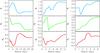 |
Fig. A.2 Same as Fig. A.1, but for the phase angle θm, in units of π rad, with m = 1,2,3. |
| In the text | |
|
Fig. A.3 Gravitational potential of the spherical stellar bulge of M 99, in units of 103 km2 s-2. |
| In the text | |
|
Fig. A.4 Amplitude vk of the kinematical Fourier mode k for the observed velocity field of M 99 in units of km s-1. |
| In the text | |
Current usage metrics show cumulative count of Article Views (full-text article views including HTML views, PDF and ePub downloads, according to the available data) and Abstracts Views on Vision4Press platform.
Data correspond to usage on the plateform after 2015. The current usage metrics is available 48-96 hours after online publication and is updated daily on week days.
Initial download of the metrics may take a while.