| Issue |
A&A
Volume 588, April 2016
|
|
|---|---|---|
| Article Number | A116 | |
| Number of page(s) | 16 | |
| Section | The Sun | |
| DOI | https://doi.org/10.1051/0004-6361/201527475 | |
| Published online | 28 March 2016 | |
Constraints on energy release in solar flares from RHESSI and GOES X-ray observations
II. Energetics and energy partition
Leibniz-Institut für Astrophysik Potsdam (AIP),
An der Sternwarte 16,
14482
Potsdam,
Germany
e-mail:
This email address is being protected from spambots. You need JavaScript enabled to view it.
Received: 29 September 2015
Accepted: 16 February 2016
Abstract
Aims. We derive constraints on energy release, transport and conversion processes in solar flares based on a detailed characterization of the physical parameters of both the thermal plasma and the accelerated nonthermal electrons based on X-ray observations. In particular, we address the questions of whether the energy required to heat the thermal plasma can be supplied by nonthermal particles, and how the energetics derived from X-rays compare to the total bolometric radiated energy.
Methods. Time series of spectral fits and images for 24 flares ranging from GOES class C3.4 to X17.2 were obtained using RHESSI hard X-ray observations. This has been supplemented by GOES soft X-ray fluxes. In our companion Paper I, we have used this data set to obtain the basic physical parameters for the thermal plasma (using the isothermal approximation) and the injected energetic electrons (assuming the thick-target model). Here, we used this data set to derive the flare energetics, including thermal energy, radiative and conductive energy loss, gravitational and flow energy of the plasma, and kinetic energy of the injected electrons. We studied how the thermal energies compare to the energy in nonthermal electrons, and how the various energetics and energy partition depend on flare importance.
Results. All flare energetics show a good to excellent correlation with the peak GOES flux. The gravitational energy of the evaporated plasma and the kinetic energy of plasma flows can be neglected in the discussion of flare energetics. The radiative energy losses are comparable to the maximum thermal energy, while the conductive losses are considerably higher than the maximum thermal energy, especially in weaker flares. The total heating requirement of the hot plasma amounts to ≈50% of the total bolometric energy loss, with the conductive losses as a major contribution. The nonthermal energy input by energetic electrons is not sufficient to account for the total heating requirements of the hot plasma or for the bolometric losses, in particular in weak flares.
Conclusions. Our results support the standard model of solar flares, with the following modifications. (1) Heating the hot thermal plasma and supplying the bolometric radiated energy requires an additional non-beam heating mechanism. (2) Strong conductive losses are a necessary additional energy transport process that transfers the energy released in the corona to the lower (and denser) atmospheric layers, where the bulk of the released energy is efficiently radiated away at longer wavelengths (EUV, UV, and white light) by cooler material.
Key words: Sun: flares / Sun: X-rays, gamma rays / acceleration of particles
© ESO, 2016
1. Introduction
Characterizing the energy partition is a crucial prerequisite for a physical understanding of solar flares, or indeed of any physical system. In the most basic form of the standard flare model (the CSHKP model of eruptive solar flares; cf. Carmichael 1964; Sturrock 1966; Hirayama 1974; Kopp & Pneuman 1976), energy release, transport, and conversion processes are very simple. Triggered by magnetic reconnection, stored magnetic energy is released and converted mainly into kinetic energy of nonthermal particles by some form of acceleration mechanism. The particle beams formed in this way then deposit their energy in the dense chromosphere, triggering chromospheric evaporation that fills the flare loops with hot X-ray emitting plasma (T> 10 MK). This scenario is strongly supported by the Neupert effect (Neupert 1968). Finally, the hot plasma loses energy due to radiation and conduction.
Many attempts have been made to determine whether the energy partition in solar flares (in particular the ratio between thermal and nonthermal energy) is consistent with this simple standard model. Quantitative measurements of the nonthermal energy input by accelerated electrons (and, to a lesser degree, also ions) have become available with the hard X-ray (HXR) instrument Ramaty High Energy Solar Spectroscopic Imager (RHESSI; Lin et al. 2002), using the thick-target model of Brown (1971). In contrast, the thermal energetics have been derived from a much wider range of data sources and spectral models. GOES soft X-ray fluxes have been used extensively with an isothermal model (e.g., Veronig et al. 2005; Emslie et al. 2012). Other studies have employed HXR spectroscopy with RHESSI, usually assuming an isothermal model (e.g., Saint-Hilaire & Benz 2005; Caspi et al. 2014a). Only a few attempts have been made to fit the HXR spectra with bithermal (Caspi & Lin 2010) or multithermal components (Aschwanden 2007; Jain et al. 2011). Recently, the quantitative characterization of multithermality has become possible with differential emission measure distributions (DEMs) derived from a new generation of extreme ultraviolet (EUV) multi-filter imagers (SDO/AIA) as well as spectrographs (SDO/EVE, Hinode/EIS) that provide the required spectral resolution and coverage. Now these DEMs are starting to be used to obtain thermal energies (Aschwanden et al. 2015).
Most studies have concluded that the energy in nonthermal electrons is sufficient to generate the thermal component, which is consistent with the standard model of solar flares (cf. Saint-Hilaire & Benz 2002, 2005; Holman et al. 2003; Emslie et al. 2004, 2005, 2012). However, it is very difficult to compare and evaluate these studies because of their different approaches in terms of data sources and model assumptions for the thermal component (see discussion above), as well as event selection criteria. In addition, radiative and especially conductive losses have only rarely been considered (for counter-examples, see, e.g., Veronig et al. 2005; Fletcher et al. 2013).
In the light of the problems discussed above, we try to constrain energy release, transport, and conversion processes, as well as electron acceleration, by a comprehensive characterization of the basic physical parameters in a larger number of flares, thus bridging the gap between individual case studies and large statistical studies. We have analyzed 24 RHESSI flares in detail (ranging from weak C-class to strong X-class events), deriving time series of spectral fits and HXR images for each of them. The source sizes have already been studied in Warmuth & Mann (2013a,b). In Warmuth & Mann (2016), henceforth Paper I, we have added spectroscopic information from RHESSI and GOES to determine a wide range of physical parameters of the thermal plasma and the accelerated electrons. The most important result from this study was that the flare plasma is multithermal in nature and consistent with a bi-modal distribution: a cooler plasma component (≈10–25 MK) that is generated by chromospheric evaporation, and an additional hotter component (T> 25 MK) that is more consistent with direct in situ heating of coronal plasma. The second component is observable only with RHESSI and not with GOES, since GOES is not sensitive to temperatures above 25 MK. The presence of this multithermal plasma, combined with the different temperature responses of RHESSI and GOES, is the reason for the systematic differences of the plasma parameters derived from the two instruments.
In this paper, we use the parameters obtained in Paper I to study the energy partition in solar flares, with the aim of better understanding energy release, transport, and conversion processes in solar flares. After briefly describing the observations and analysis techniques (Sect. 2), we investigate how the different flare energetics scale with various physical parameters (Sect. 3). Then we study the energy partition in solar flares in detail, including how thermal and nonthermal energies scale with each other, and how all energetics scale as a function of GOES importance (Sect. 4). The results are discussed in Sect. 5, and the conclusions are given in Sect. 6.
2. Observations
For our study of energetics, we have selected 24 flares from GOES class C3.4 to X17.2 (seven C-class, eight M-class, and nine X-class), the same sample used in the geometric study of Warmuth & Mann (2013a,b) and in Paper I. In the latter paper, the event selection criteria and analysis techniques are discussed in detail, therefore we give here only a brief overview. We note that many of the events have been used previously for comparison with a shock-drift acceleration model (Mann et al. 2009; Warmuth et al. 2009b) and for the study of nonthermal energetics in the framework of magnetic reconnection (Mann & Warmuth 2011). All flares show a pair of nonthermal HXR footpoints. Most of the events are eruptive, and there are no gradual or long-duration events in our sample.
We have obtained time series of RHESSI HXR spectra for all events. Using the OSPEX package1, the spectra were fitted with an isothermal component plus a nonthermal thick-target bremsstrahlung component given by a power-law electron distribution (Brown 1971). These fits yield emission measure EM and temperature T of the thermal plasma and also the total flux of injected nonthermal electrons Fnth, spectral indices δL and δH below and above the break energy EB, and low-energy cutoff EC. For the thermal component, the HXR spectra were supplemented by SXR fluxes from the GOES X-ray Sensor (XRS), which yield EM and T using the code developed by White et al. (2005). We denote the quantities derived from RHESSI with the suffixes R and G throughout (e.g., TR and TG). Finally, the spectra were complemented by time series of RHESSI HXR images that were used to determine the volume Vth of the thermal plasma and the total nonthermal footpoint area Anth,tot.
From this parameter set, we derived the relevant energetics. Starting with the thermal plasma, we obtained the thermal energy as a function of time t by  (1)with k as Boltzmann’s constant and f the filling factor. Here, we adopted f = 1, which implies that the thermal energies are upper limits. The validity of this assumption is discussed in Sect. 5.2.
The maximum thermal energy is only a lower limit for the amount of energy that is required to generate and sustain the thermal plasma. Energy losses due to radiation and conduction have to be accounted for as well. For the radiative energy loss rate Prad(t), we used the radiative loss rates given by the CHIANTI package (Dere et al. 1997; Landi et al. 2013). The conductive loss rate of the hot plasma through the two footpoints is estimated by  (2)with the classical Spitzer coeffcient for thermal conduction, κ0 = 10-6 erg cm-1 s-1 K−7/2, and (dFPπ) / 4 as the loop half-length (assuming a semicircular loop with the footpoint separation dFP as diameter), which we adopted as the temperature scale length (cf. Phillips et al. 1996; Veronig et al. 2005). Since this conductive flux usually saturates under typical flare conditions, we adopted the approach of Battaglia et al. (2009) to reduce the fluxes appropriately. The total radiative and conductive losses, Erad and Econd, were obtained by integrating over the event duration. The durations were defined by the availability of good RHESSI spectroscopy (cf. Paper I), and while the impulsive phase was fully covered in all events, the late or gradual phase of many events was cut short by the occurrence of RHESSI night times. Erad and Econd are therefore lower limits, but we do not expect them to be significantly lower than they would be for longer integration times. The radiated energies derived by Ryan et al. (2012), who used longer integration times, are comparable to our values. Accordingly, the conductive losses are very low in the late phase because of the lower temperatures.
Accordingly, the kinetic energy of the injected electrons Enth results from integrating the kinetic power Pnth (obtained from the spectral parameters of the thick-target fits) over time. We note that since the low-energy cutoff EC is usually masked by the thermal component, we adopted the highest cutoff that is consistent with the data. Therefore, our nonthermal fluxes, powers, and energies are lower limits. The implications of this is discussed in Sect. 5.5.
Table 1 lists all events in ascending order of GOES importance. In addition to flare number, IAU event identifier (which gives the event date and the time of peak GOES flux), and GOES class, the table gives the maximum thermal energies as derived from RHESSI and GOES, Eth,R and Eth,G, radiative energy loss of the hot plasma, Erad,R and Erad,G, conductive energy loss, Econd,R and Econd,G, total energy required for heating the thermal plasma, Eh (see Sect. 5.4), and nonthermal energy input by electrons, Enth.
3. Scaling of energetics with physical parameters
In Sect. 4 of Paper I, we have studied how the maxima of various thermal and nonthermal parameters scale with GOES importance. In the following, we investigate how the maximum thermal energies, energy loss rates, and nonthermal energy input rates depend on the various physical parameters.
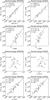 |
Fig. 1 Maximum thermal energies Eth derived from RHESSI (left column) and GOES (right column) as a function of the emission measure EM (top row), temperature T (2nd from top), electron density n (3rd from top), and thermal volume Vth (bottom row). We also show power-law fits obtained with the BCES bisector method (full black line). The slope α and intercept b of the obtained power law and the rank correlation coefficient R are indicated. |
Energetics of the 24 flares.
3.1. Scaling of thermal energetics
Figure 1 shows the maximum thermal energy Eth derived from RHESSI and GOES as a function of the co-temporal emission measure, temperature, electron density, and thermal volume. We also show power-law fits obtained with the Bivariate Correlated Errors and intrinsic Scatter (BCES) bisector estimator (Akritas & Bershady 1996), a method based on performing two weighted linear least-squares regression fits on the data, or on the logs of the data – log x on log y and log y on log x (for a more detailed discussion, see Warmuth & Mann 2013b). The bisector is obtained as log y = b + αlog x, and the corresponding power law is  (3)with α as the slope and b as the intercept.
For both RHESSI and GOES, the maximum thermal energies show excellent correlation with the emission measure (with rank correlation coefficient R ≥ 0.92) and good correlation with the temperature (R = 0.68). While the relation with EM is nearly linear (α ≈ 1), the temperature dependency is highly nonlinear and very steep (α> 5). Separating EM into density and volume, we find that the maximum thermal energies are only very weakly dependent on density, while there is a clear linear dependency on volume (R = 0.88). Considering not the maximum thermal energy, but Eth at the time of peak GOES flux, gives similar results, with the exception of the relation to density, where now a modest correlation is found (R = 0.33 and R = 0.5 for RHESSI and GOES, respectively). However, the basic conclusions on Eth remain the same: thermal energy strongly depends on temperature and source volume, and is – at best – only moderately dependent on plasma density. Eth derived from RHESSI and GOES shows very similar dependencies, with the exception of temperature, for which Eth,G rises more steeply than Eth,R, which is a result of the more shallow increase of GOES temperatures discussed in Paper I.
The dependencies of the maximum radiative energy loss rates Prad are plotted in Fig. 2. As for Eth, Prad shows excellent correlation with co-temporal emission measure (R ≥ 0.97), and reasonable correlation with temperature (R ≥ 0.64). In contrast to Eth, the maximum radiative loss rates show a moderate correlation both with plasma density (R ≥ 0.6) and volume (R ≥ 0.54). Again, considering Prad at the GOES peak times gives very similar results, and RHESSI and GOES show no significant differences apart from the relation with temperature.
Finally, Fig. 3 depicts the correlations of the maximum conductive energy loss rates Pcond with several parameters. The correlation with emission measure is lower (R = 0.58 and 0.52) than in the case of the thermal energies or radiative loss rates, which is not surprising since EM does not enter explicitly into the calculation of the conductive losses. As expected, Pcond is highly correlated with temperature (R = 0.82). The correlation with plasma density is modest (R = 0.3 and 0.52), and there is only a very weak correlation with total footpoint area (R = 0.18 and 0.14). The correlation with footpoint separation (not shown here) is equally weak. We conclude that the conductive losses are overwhelmingly determined by temperature.
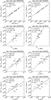 |
Fig. 2 Maximum radiative loss rates Prad derived from RHESSI (left column) and GOES (right column) as a function of the emission measure EM (top row), temperature T (2nd from top), electron density n (3rd from top), and thermal volume Vth (bottom row). |
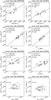 |
Fig. 3 Maximum conductive loss rates Pcond derived from RHESSI (left column) and GOES (right column) as a function of the emission measure EM (top row), temperature T (2nd from top), electron density n (3rd from top), and nonthermal footpoint area Anth,tot (bottom row). |
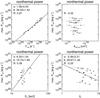 |
Fig. 4 Maximum kinetic power Pnth of nonthermal electrons as a function of the electron flux Fnth (top left), nonthermal footpoint area Anth,tot (top right), low-energy cutoff EC (bottom left), and electron spectral index δL (bottom right). |
3.2. Scaling of nonthermal energetics
Figure 4 shows the maximum kinetic power Pnth of the injected electrons as a function of various nonthermal parameters. While the maximum Pnth naturally shows excellent correlation with the injected electron flux, there is no correlation with the footpoint area. This lack of correlation with area implies that the flux densities have primarily to account for the wide range of nonthermal energy input rates.
Only modest correlations are found for the low-energy cutoff EC and the spectral index δL. The apparent increase of power with rising low-energy cutoff is merely a consequence of the more pronounced thermal component, as we discussed in Paper I. In contrast, previous studies have established a more pronounced anticorrelation between spectral index and photon flux (cf. Parks & Winckler 1969; Grigis & Benz 2004; Battaglia et al. 2005) or electron flux (cf. Warmuth et al. 2009b) at a fixed energy. Apparently, the correlation with total power is reduced by the influence of the low-energy cutoff, which has a strong effect on the deduced total powers. Taking the electron flux at 50 keV instead of the total power (and thus effectively removing the influence of the low-energy cutoff), we find a more pronounced anticorrelation (R = −0.55) that is consistent with the relations deduced in the earlier studies. The question remains whether the true total powers (i.e., the powers without a masked low-energy cutoff) would also show a significant anticorrelation or not.
We therefore conclude that the acceleration mechanism is able to generate electron fluxes with a wide range of magnitudes, with only a loose relation between total flux and spectral index, and without any dependency on footpoint area. The latter fact suggests that there is probably no significant dependency of the maximum electron flux on the cross-sectional area in the acceleration region (assuming that this areas is correlated with the footpoint area). The caveat here is that RHESSI imaging reaches its limits for very compact footpoints (see Warmuth & Mann 2013a), therefore a correlation with footpoint area may potentially be obscured by this effect.
4. Energy partition and scaling with flare importance
In this section, we present the partition of the different forms of flare energies. We start with the energetics of the thermal plasma, continue with the relation between thermal energies and nonthermal input, and close with the partition of energies as a function of GOES peak flux and with respect to the total energy that is released.
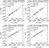 |
Fig. 5 Maximum gravitational energy, Egrav (top) and maximum kinetic flow energy, Eflow (bottom) of the hot plasma plotted versus maximum thermal energy, Eth, derived from RHESSI (left) and GOES data (right). Power-law fits (full lines), the slope α and intercept b of the obtained power law, and the rank correlation coefficient R are also indicated. The dotted line denotes x = y, and the median ratio M of the different energies is indicated. Both gravitational and flow energies are significantly lower than the maximum thermal energies. |
4.1. Gravitational energy of hot plasma and kinetic energy of plasma flows
The evaporated chromospheric plasma that fills up the flaring loops does not only have thermal energy Eth, but also gravitational (potential) energy Egrav (since it has to be transported from the chromosphere up to heights of heights some tens of Mm) and kinetic energy Eflow associated with the plasma flow. Usually, Egrav and Eflow are either not discussed in studies of flare energetics at all, or an equipartition of the three energies is assumed when estimating the total plasma energy content (e.g., Veronig et al. 2005). Here, we aim for a more accurate assessment.
The mass of the thermal plasma is  (4)where 1.92 × n is the total number density of particles for solar abundances,
  the mean molecular weight (taken as 0.6; cf. Priest 1982), and mp the proton mass. We now estimate Egrav by assuming that all thermal plasma is located at a height corresponding to half the footpoint distance dFP (i.e., at the apex of a semicircular loop). This gives
 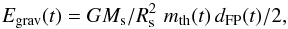 (5)where G is the gravitational constant and Ms and Rs the solar mass and radius. Assuming that all thermal plasma is streaming with the speed vflow, the kinetic energy of the streaming plasma is
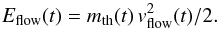 (6)In Fig. 5 (upper row) the maximum gravitational energy is plotted as a function of maximum thermal energy for RHESSI- and GOES-derived parameters. It is evident that Egrav is lower than Eth by about two orders of magnitude and can therefore be safely neglected.
Determining the kinetic flow energy is more difficult, since we need to know the flow speed in addition to our spectral and geometric parameters. With SOHO/CDS, spatially resolved upflows with peak speeds in the range of 70–200 km s-1 have been observed in the Fe xix line (Czaykowska et al. 1999; Teriaca et al. 2003; Brosius & Phillips 2004; del Zanna et al. 2006; Milligan et al. 2006), which is formed at T = 8 MK. More recently, Brosius (2013) has measured peak upflow speeds of 200 km s-1 in the hotter Fe xxiii line (T = 14 MK) with Hinode/EIS. Speeds of 30–300 km s-1 have been reported from recent observations with IRIS (cf. Brosius & Daw 2015; Battaglia et al. 2015; Graham & Cauzzi 2015; Sadykov et al. 2015).
We therefore adopted 200 km s-1 as our flow speed, which probably results in an overestimation of the kinetic energies, since the speeds given above are peak speeds. The resulting maximum Eflow is plotted versus maximum Eth in Fig. 5 (lower row). While Eflow is higher than Egrav, it still amounts to only ≈5% of Eth on average. A flow speed of ≈700 km s-1 would be required to have equipartition between thermal and kinetic flow energy; this value is clearly not supported by observations.
We thus conclude that we can neglect both the gravitational energy and the kinetic flow energy of the hot plasma in our discussion of flare energetics.
4.2. Energy losses of the hot thermal plasma
The amount of energy input that is required to generate the hot thermal plasma is not determined by the maximum thermal energy alone. The energy losses of the plasma that are due to both radiation and conduction have to be accounted for as well. Both loss processes can be significant, with conduction dominating for T> 10 MK (see e.g., Aschwanden & Alexander 2001; Fletcher et al. 2013).
In Fig. 6 we compare the total (i.e., event-integrated) radiative energy loss Erad (upper row) and the conductive energy loss Econd (lower row) with the maximum thermal energy Eth for RHESSI- and GOES-derived parameters. All energy losses show a good correlation with the maximum thermal energy. For Erad, the slope of the power-law is larger than unity (α ≈ 1.35), which means that more energetic flares suffer proportionally higher radiative losses. We note that Emslie et al. (2012) have found a correlation with a slope that is similar within uncertainties (α = 1.29 ± 0.12), which is shown as a dash-dotted line in Fig. 6. For the RHESSI-derived parameters, Erad ≤ Eth in all events (with a median ratio of Erad/Eth = 0.29), while GOES yields Erad>Eth in the majority of cases (median ratio: 1.19). The higher radiative losses of GOES than RHESSI are explained by the corresponding higher emission measures.
The conductive energy losses show a quite different relation to the maximum thermal energy. Both RHESSI and GOES yield a power-law index below unity (α ≈ 0.7), implying that less energetic flares suffer relatively more severe conductive losses than more energetic events. For RHESSI, the conductive losses are almost an order of magnitude higher than the maximum thermal energies (median ratio Econd,R/Eth,R = 8.67). For GOES, more energetic events show comparable conductive losses and maximum thermal energies, while in weaker flares, the conductive losses also dominate (median ratio Econd,G/Eth,G = 2.45). The higher conductive losses given by RHESSI directly result from the higher RHESSI temperatures.
In summary, the RHESSI plasma is dominated by conductive losses, while the radiative and conductive losses are on the same order for the GOES plasma. The energy losses are either comparable to or higher than the maximum thermal energies, thus they are important components that cannot be neglected in the study of flare energetics. This is particularly important when investigating whether the energy input by nonthermal particles can account for the generation of the thermal flare plasma.
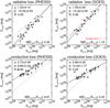 |
Fig. 6 As in Fig. 5, but showing the radiative (top) and conductive energy loss (bottom) of the hot plasma, Erad and Econd, plotted versus maximum thermal energy Eth, derived from RHESSI (left) and GOES data (right). For the radiative energy loss given by GOES, the relation derived from Emslie et al. (2012) is shown by the dash-dotted line. |
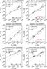 |
Fig. 7 Maximum thermal energy, Eth (top), radiative loss, Erad (middle), and conductive energy loss, Econd (bottom), of the hot plasma derived from RHESSI (left) and GOES data (right), plotted versus energy input by nonthermal electrons, Enth. For Eth,G and Erad,G, the relations derived from Emslie et al. (2012) are shown by the dash-dotted line. |
4.3. Thermal versus nonthermal energetics
After quantifying the various energetic components of the thermal plasma, we now consider the main question: is the energy input by nonthermal particles sufficient to account for the generation (and the sustainment) of the hot thermal plasma? In other words, are particle beams really the main heating mechanism in solar flares?
In Fig. 7 we compare the relevant thermal energetics (derived from RHESSI and GOES) to the total kinetic energy Enth of the injected nonthermal electrons. Two caveats have to be noted here. First, Enth are lower estimates because of the masked low-energy cutoff. Second, the energy input by accelerated ions is not considered here. The implications of these two facts are discussed in Sects. 5.5 and 5.6, respectively.
The top row of Fig. 7 shows the maximum thermal energies Eth plotted against the nonthermal input Enth. The excellent correlations (R ≥ 0.93) suggest that the hot thermal plasma is indeed closely related with the nonthermal input. Moreover, the thermal energies are lower than the nonthermal input in all events (with a median fraction of Eth/Enth ≈ 0.3), which suggests that the electron beam could indeed generate the hot thermal component. However, the power-law index is below unity (α ≈ 0.8), therefore the thermal and nonthermal energies become comparable in weak flares. When taking Eth,G and Enth derived for the sample of Emslie et al. (2012), a very similar relation is found (cf. the dash-dotted line in Fig. 7).
We continue with the radiative energy loss Erad (middle row of Fig. 7), which again shows excellent correlation (R ≥ 0.9) with Enth. The scalings are close to linear, and the median ratios of radiative loss over nonthermal input are 0.08 for RHESSI and 0.33 for GOES. So far, we have shown that both the maximum thermal energy and the radiative energy loss can be easily accounted for by the injected electrons. This is consistent with the results of Emslie et al. (2012) (cf. the dash-dotted lines in Fig. 7). However, the correlation found by the latter study was significantly lower than in our case.
We now turn to the conductive energy losses Econd, for which we provide the first systematic study of its correlation with the nonthermal energy input (see bottom row of Fig. 7). The scaling of conductive energy loss with nonthermal input is consistent with a power law with a slope below unity (α = 0.58 and 0.54 for RHESSI and GOES, respectively), which reflects what we have found for its relation with maximum thermal energy in Sect. 4.2. For RHESSI, the conductive losses are clearly higher than the energy input by electrons in the majority of flares (with a median ratio Econd,R/Enth = 1.45). This is particularly pronounced in the less energetic events. In contrast, the conductive losses given by GOES are lower than the nonthermal input for more energetic events, with a median ratio Econd,G/Enth = 0.61.
We have thus shown that the nonthermal energy input by electrons cannot offset the conductive losses of the hot plasma, at least not when considering less energetic flares, or when calculating the conductive losses using RHESSI-derived thermal parameters. This contrasts strongly with all other thermal energetics, which can be easily supplied by the nonthermal electrons. The nonthermal input could of course be higher in case of a lower low-energy cutoff (see Sect. 5.5) or a contribution by accelerated ions (Sect. 5.6). Other problems related with the conductive losses are discussed in Sect. 5.8.
4.4. Total radiated energy
So far, we have only discussed energetics based on SXR and HXR observations. However, flares are known to radiate energy basically over the whole electromagnetic spectrum, therefore we have only gained partial insight into the energy partition in solar flares. In particular, flares emit large amounts of energy in the EUV, UV, and white-light (WL) range. Early estimates for the total radiant energy were around ten times the energy emitted in SXRs (e.g., Neidig 1989).
Any meaningful constraints on the energy partition in solar flares can only be made if the total amount of energy that is released in a flare is determined first. Assuming that after various conversion processes (particle acceleration, generation of flows, heating) all the released energy will finally be thermalized and radiated away, the total bolometric radiated energy Ebol (i.e., the radiative energy loss summed over all wavelengths) is a measure for this total released energy2.
The total energy radiated by a flare has first been measured directly in the total solar irradiance (TSI) data obtained with the SORCE/TIM instrument (Kopp & Lawrence 2005) by Woods et al. (2004). Woods et al. (2006) reported Ebol for four strong X-class flares (i.e., ≥X10). Here, we adopted the corresponding values from Emslie et al. (2012), who have corrected these bolometric energies for limb-darkening absorption and added an event studied by Moore et al. (2014). Thus we obtain total radiated energies of 1.4–3.6 × 1032 erg in very strong flares.
This technique can only be applied to strong flares because the TSI flare signal is usually much weaker than the background fluctuations of the TSI. However, a superposed-epoch analysis can be performed to obtain Ebol for a larger ensemble of weaker flares. Kretzschmar et al. (2010) have applied this technique to the SOHO/VIRGO data set (Fröhlich et al. 1997) from 1996 to 2008 and found statistically significant bolometric flare energies even for C-class flares.
In Fig. 8 we plot Ebol as given by Kretzschmar (2011) for flare ensembles with different mean X-ray importance (from C8.7 to X3.2). We note that as a function of peak GOES flux, Ebol closely agrees with a power law with a slope of α = 0.79 ± 0.11 and an intercept of b = 34.5 ± 0.5 (rank correlation coefficient R = 1). A slope smaller than unity means that the total radiated energy rises at a significantly lower rate than the peak GOES flux. Second, we point out that the power law intersects the individual bolometric energies measured by SORCE/TIM. Thus the two different methods (and instruments) give consistent results, at least for strong flares.
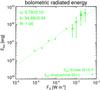 |
Fig. 8 Total (bolometric) radiated energies, Ebol, in solar flares as a function of peak GOES flux FG, as given by Emslie et al. (2012, diamonds) and Kretzschmar (2011, crosses). A power-law fit (dotted line) to the values of Kretzschmar (2011), its slope α and intercept b, and the rank correlation coefficient, R, are also shown. |
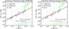 |
Fig. 9 Maximum thermal energy, Eth (dots), as a function of the background-subtracted peak GOES flux FG, derived from RHESSI (left) and GOES data (right). We also indicate a power-law fit (full black line) of Eth , the slope α and intercept b of the obtained power law, and the rank correlation coefficient R. The corresponding relations derived by Caspi et al. (2014a) and Emslie et al. (2012) are shown as blue and red dash-dotted lines, respectively. For comparison, the total (bolometric) radiated energies, Ebol, as derived by Emslie et al. (2012, diamonds) and Kretzschmar (2011, crosses), are also shown. The dotted green line shows a power law fitted to Ebol as derived by Kretzschmar (2011). |
Both methods find that only 1% of the energy is emitted in X-rays, ≈50% in EUV (which is emitted both by coronal flare loops and chromospheric ribbons), and ≈50% in near-UV, white light, and infrared (emitted from the lower atmospheric layers, i.e., chromosphere and photosphere).
We therefore conclude that we have a fairly good estimate of the total energies released in solar flares. These total energies are on the order of 1030 erg for C-class flares and rise to several 1032 erg for very strong X-class flares. A significant fraction of the energy is emitted by comparatively cool and dense material in low atmospheric layers. In the following, we study how the energetics derived from X-rays compare to the bolometric energies.
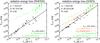 |
Fig. 10 As in Fig. 9, but showing the radiative energy loss, Erad (dots), as a function of peak GOES flux FG, derived from RHESSI (left) and GOES data (right). The corresponding relations derived by Ryan et al. (2012) and Emslie et al. (2012) are shown as orange and red dash-dotted lines, respectively. |
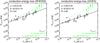 |
Fig. 11 As in Fig. 9, but showing the conductive energy loss, Econd (dots), as a function of peak GOES flux FG, derived from RHESSI (left) and GOES data (right). |
4.5. Energetics as a function of flare importance
4.5.1. Thermal energy
Our comparison of flare energetics derived from X-rays with the total released energy as a function of GOES importance FG starts with the maximum thermal energy of the hot plasma, Eth, which is shown in Fig. 9 for both RHESSI- and GOES-derived thermal parameters. As in Paper I, FG refers to the background-subtracted peak fluxes. Both Eth,R and Eth,G are excellently correlated with the peak GOES flux (R ≥ 0.94), and the relation can be represented by power laws with very similar slopes of α = 0.86 and 0.88, respectively. These power laws are slightly steeper, but generally consistent with what was reported in previous studies. Caspi et al. (2014a) found α = 0.64 ± 0.07 for the RHESSI thermal energies, or α = 0.78 ± 0.07 when using the BCES method which is shown in Fig. 9. For the GOES-derived thermal energies Emslie et al. (2012) obtained α = 0.74 ± 0.09. Compared to the bolometric radiated energies, we find that the maximum thermal energies are more than an order of magnitude lower (Ebol/Eth = 12−28), but they do show a comparable slope.
4.5.2. Radiative energy loss of the hot plasma
Figure 10 shows the radiative energy loss of the hot plasma, Erad, as derived from RHESSI and GOES. Again, the energies are well correlated with the GOES peak flux (R ≥ 0.92) and can be represented as power laws. In contrast to Eth, the slopes are above unity (α = 1.16 and α = 1.18 for RHESSI and GOES, respectively). Erad is one to two orders of magnitude lower than Ebol, which clearly shows that the total radiated energy in solar flares has to contain a significant contribution by emission from cooler material (i.e., T< 5 MK; cf. Woods et al. 2004, 2006; Kretzschmar 2011). For RHESSI, the radiated energies are lower than the total radiated energies by a factor of 30–360, and by a factor of 5–65 for GOES.
The radiative energies derived by Emslie et al. (2012) are higher than ours and have a slope below unity (α = 0.89 ± 0.12). In contrast, the energies derived by Ryan et al. (2012) for a large sample of GOES flares are also higher than ours (by a factor of ≈3), but they do show a very similar slope (α = 1.2 ± 0.004). There are several potential reasons for these discrepancies. One problem might be that different integration times are used in the various studies. We restricted the integration time to the time range of clearly detectable HXR emission, which can be cut short in comparison to GOES by background problems and RHESSI spacecraft nights. In this sense, our radiated energies are lower estimates. A second important effect is event selection. While Emslie et al. (2012) have focused on eruptive M and X-class flares, Ryan et al. (2012) have included all GOES flares from class A upwards. We compared our radiative energies with those from Ryan et al. (2012) for the events that are included in both studies (19 out of 24). While the radiated energies can differ by factors of up to 2 for individual events, the relation of Erad,G with GOES peak flux using the Ryan et al. (2012) values is almost identical with our result. We thus conclude that event selection is indeed the most important reason for the apparent discrepancies in the Erad,G − FG relation. Most likely, our lower values for the radiative energies stem from the absence of gradual and long-duration events in our sample.
4.5.3. Conductive energy loss of the hot plasma
The conductive energy losses obtained from RHESSI and GOES as a function of GOES peak flux are plotted in Fig. 10. As for Eth and Erad, Econd shows very good correlation with FG (R ≥ 87). However, the fitted power laws have significantly smaller slopes than for the other energies, namely α = 0.63 and 0.58 for RHESSI and GOES, respectively. The conductive losses are also lower than the bolometric radiated energies, but by less than an order of magnitude. For weaker flares and particularly for the RHESSI-derived values, Econd becomes comparable to Ebol. This indicates that the conductive losses (which are considered here for the first time for a larger event sample) play a very important role in terms of flare energetics and hence are crucial for our understanding of flare physics in general. We discuss this matter in Sect. 5.8 in more detail.
4.5.4. Nonthermal electron energy input
After discussing the energetics of the thermal plasma, we conclude our study of energetics as a function of GOES importance with the kinetic energy in nonthermal electrons, Enth, which is shown in Fig. 12. Enth shows an excellent correlation with GOES peak flux (R = 0.96) that can be represented by a power law with slope α = 1.08 (i.e, a relation close to linear). A rather similar relation can be obtained for the values derived by Emslie et al. (2012), albeit with a larger uncertainty (α = 0.98 ± 0.23). The nonthermal energies are lower than the bolometric energies in all studied events. However, the steeper slope of the Enth − FG relation implies that while Enth is about an order of magnitude lower than Ebol for C-class flares, Enth becomes comparable to Ebol for extremely strong flares. Taken at face value, this would imply that the nonthermal particles are not sufficient to account for the total energy released in a solar flare. However, we emphasize that Enth is only a lower estimate because the low-energy cutoff is unknown and also because it does not include the contribution of accelerated ions. These problems are discussed in more detail in Sects. 5.5 and 5.6.
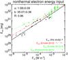 |
Fig. 12 As in Fig. 9, but showing the total injected energy in nonthermal electrons, Enth (dots), as a function of peak GOES flux FG. The red dash-dotted line indicates the relation derived by Emslie et al. (2012). |
5. Discussion
5.1. Energies as a function of GOES peak flux
In the previous section we have found that all relevant flare energetics – maximum Eth, Erad, Econd, and Enth – show a good correlation with peak GOES flux that is well represented by power laws. When the respective relations were studied previously, our results generally agree with those studies. However, we find stronger correlations in some cases, which could be due to several reasons. In contrast to most other studies, we included flares from a wide range of GOES peak fluxes. Our event sample may be more homogeneous than in other cases because one of the event selection criteria was that two nonthermal footpoints had to be observed and that the thermal source had to be not too complex or fragmented. As a result, the flares in our sample tend to be more impulsive than average, with a high association with eruptive activity and a lack of gradual events (cf. Warmuth & Mann 2013a). Finally, we made a great effort to determine the HXR source sizes (cf. Warmuth & Mann 2013a,b), which should lead to more reliable thermal energies and conductive losses.
5.2. Filling factor of thermal and nonthermal sources
We have used the common assumption of a filling factor of unity (f = 1) for both the thermal volume and the footpoint area. In this sense, our thermal energies and conductive energy losses are upper limits (we note that the radiative losses are not dependent on the filling factor). The problem of filling factors has been widely discussed in the literature. In particular, the validity of the assumption f = 1 has been called into question, with studies suggesting f< 0.1 (e.g., Cargill & Klimchuk 1997). Applying a fractal geometry model to a set of flares observed with TRACE, Aschwanden & Aschwanden (2008) have derived very low volume filling factors, ranging from 0.03–0.08 at flare peak to values as low as 0.001 in the early phase. In contrast to this, Jakimiec & Ba¸k-Stȩślicka (2011) have deduced a mean filling factor of 0.9 from the EM–T evolution of 20 flares observed with Yohkoh/SXT. Most recently, Guo et al. (2012) have used HXR imaging spectroscopy data of 22 extended-loop events with a collisional energy loss model to derive filling factors between 0.1 and unity.
Given the wide range of values for f in the literature, what would be the consequences of adopting a smaller filling factor for our events? This would reduce the thermal energies by a factor of f− 1 / 2 and the conductive losses by ≤f-1, while the electron densities would increase by f1 / 2. This leads to several problems.
We first consider electron densities. A direct measurement of electron densities is possible with density-sensitive EUV line ratios, which removes the need to determine volumes and filling factors. Most of these studies have used lines that are formed at cooler temperatures (i.e., 1–2 MK) than the hot plasma considered in this study. First reliable measurements for plasmas of ≈10 MK were reported by Mason et al. (1984), who derived an electron density of 4 × 1011 cm-3 from Fe xxi line ratios. Using observations with higher temporal and spectral resolution, Phillips et al. (1996) obtained densities of 2–3 × 1012 cm-3 from Fe xxi line ratios, and a very high density of 1013 cm-3 from Fe xxii ratios. Recently, Milligan et al. (2012) have used Fe xxi line ratios observed with SDO/EVE to determine electron densities of >10 MK plasmas. They found maximum densities of 1.6 × 10¹¹–1.3 × 1012 cm-3 in four X-class flares. These values are consistent with our GOES-derived densities for f = 0.5–1, which does not support the notion of very low filling factors.
Another argument against low filling factors comes from the fact that the hot plasma has to be contained by the magnetic field, which means that the magnetic pressure pm has to be higher than the gas pressure pg (i.e., a plasma beta of βp< 1). Since pg scales with f− 1 / 2, low filling factors require stronger magnetic fields. For f = 1, we already require minimum field strengths at gas pressure peak of BR = 70–280 G and BG = 90–370 G for the RHESSI and GOES plasma, respectively. Comparable results have been obtained by Caspi et al. (2014a). Adopting a filling factor of f = 0.01 would imply field strengths of up to 1000 G. This is inconsistent with various radio observations that give loop-top field strengths from several ten (Aurass et al. 2005; Rausche et al. 2007; Krucker et al. 2010) up to a few 100 G (White et al. 2003; Qiu et al. 2009).
Taking our results and the various studies discussed above into account, we conclude that the filling factors cannot be lower than 0.1 and are more consistent with unity. In terms of energetics, adopting f = 0.1 as the lowest possible value would lead to a decrease of thermal energies by a factor of  , while applying f = 0.1 to the area filling factor of the footpoints as well would lower the conductive energy loss by almost an order of magnitude. This would be just sufficient for the nonthermal energy input to replenish the conductive losses even in C-class flares. However, in this scenario sufficient energy cannot be transferred from the corona to the lower atmospheric layers to explain the observed total radiated energies. In this case, a local energy release in the chromosphere would be required (see, e.g., Fletcher & Hudson 2008).
5.3. Nonisothermality of the thermal plasma
RHESSI gives systematically higher temperatures and lower emission measures than GOES, a well-known phenomenon (e.g., Battaglia et al. 2005; Veronig et al. 2005; Sui et al. 2005) that we have investigated in detail in Paper I. RHESSI is more sensitive to high-temperature plasmas (T> 10 MK) while GOES has a broader temperature response that is more weighted to lower temperatures, which means that this result implies the presence of a multithermal plasma. Such a configuration can be quantified by the differential emission measure (DEM), and recent EUV observations have confirmed that broad DEM distributions are common in solar flares (cf. Fletcher et al. 2013; Graham et al. 2013; Kennedy et al. 2013; Warren et al. 2013; Caspi et al. 2014b; Ryan et al. 2014; Aschwanden et al. 2015).
The notion of a truly isothermal plasma is at odds with the standard flare model, where field lines are successively reconnected and filled with evaporated hot plasma, which subsequently cools down. Thus, at any given time there will be flaring loops of different temperatures, and the shape of the DEM distribution will be determined by the interplay of the various heating and cooling processes. A brief very impulsive energy input will result in a narrow DEM, which is close to the isothermal case, while a flare with a longer and more structured energy input phase will result in a broader and more complex DEM.
The scenario discussed above applies to the evaporated component that fills the coronal loop. However, DEM distributions can show even more complexity due to additional physically different plasma components. In Paper I, we have found evidence for a super-hot (T> 25 MK) thermal component that is more consistent with directly heated coronal plasma. This component is only seen by RHESSI and is present alongside the cooler (T = 10–25 MK) evaporated component. GOES observes only the evaporated plasma, while both components contribute to the RHESSI signal. Observationally, the two components are thus not completely separated by RHESSI and GOES, except for the early flare phase where there is little evaporated plasma and the RHESSI response is dominated by the directly heated plasma. If the components were totally separated, the total energies could be obtained by simply adding the energies derived from RHESSI and GOES. This will give an upper estimate for the total energy of the plasma above ≈5 MK.
We know from EUV observations that a significant part of the DEM extends to temperatures T< 5 MK, which is below the GOES temperature range. Therefore, the total thermal and radiative energies of the flare plasma have to be higher than derived from GOES and RHESSI. Generally, the isothermal assumption will underestimate the thermal and radiative energies, in particular if a significant part of the DEM is outside the instrument temperature response. Recently, Aschwanden et al. (2015) have derived the thermal energies for 400 M and X-class flares using DEMs derived from AIA multi-filter observations in the EUV. They found that using the isothermal assumption underestimates the thermal energy by a factor of ≈14 compared to the multithermal case. Applying this factor to our thermal energies would bring them into the order of the bolometric radiated energies.
5.4. Total energy requirements of the thermal plasma
We showed that thermal energies as well as radiative and conductive energy losses can behave quite differently with respect to GOES class, often dependent on whether they are derived from RHESSI or GOES. In Paper I, we have concluded that RHESSI is able to detect a super-hot coronal component that is presumably heated directly in the corona, while GOES only sees the cooler (T ≤ 25 MK) evaporated component. To finally settle the question of whether the nonthermal energy input is sufficient for generating and sustaining the hot plasma and how this relates to the total released energy in a flare, we have to estimate the total amount of energy that is required for heating the X-ray emitting plasma, Eh. Merely summing the different energy components would result in some double-counting, therefore we integrated the time derivative of the thermal energies and the loss rates over time according to 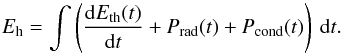 (7)In addition, we account for the fact that RHESSI and GOES observe two distinct thermal components, even though they are not always clearly separated (see discussion in Paper I). We estimate the total thermal energy to
 ![Mathematical equation: \begin{equation} E_\mathrm{th}(t)= \left[ E_{\mathrm{th},\rm R}(t) + E_{\mathrm{th},\rm G}(t) \right] \sqrt{0.5}, \end{equation}](/articles/aa/full_html/2016/04/aa27475-15/aa27475-15-eq155.png) (8)which follows from assuming a filling factor of 0.5 for both components (i.e., the volume is half filled by each component). For the radiative loss, we take
(8)which follows from assuming a filling factor of 0.5 for both components (i.e., the volume is half filled by each component). For the radiative loss, we take  (9)Finally, for the conductive loss we adopt
 ![Mathematical equation: \begin{equation} P_\mathrm{cond}(t)= 0.5 \left[ P_{\mathrm{cond},\rm R}(t) + P_{\mathrm{cond},\rm G}(t) \right], \end{equation}](/articles/aa/full_html/2016/04/aa27475-15/aa27475-15-eq157.png) (10)which assumes that half of the footpoint area is connected to each plasma component.
(10)which assumes that half of the footpoint area is connected to each plasma component.
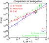 |
Fig. 13 As in Fig. 9, but showing the total energy required for heating the hot thermal plasma, Eh (red dots), as a function of peak GOES flux FG. For comparison, the energy in nonthermal electrons Enth (blue dots) and the total radiated energy Ebol (green crosses and diamonds) is shown. |
The resulting total heating energy Eh is plotted as a function of peak GOES flux in Fig. 13, together with the nonthermal energy in electrons Enth and the total radiated energy Ebol. We note that Eh agrees more closely with Ebol than any other energy considered thus far. The power-law index of the relation (α = 0.73) is close to the one of Ebol (α = 0.79), while on average Eh is lower than Eh by a factor of ≈2. In other words, ≈50% of the total radiated energy (and thus probably also of the released energy in the flare) are due to the X-ray emitting plasma – less due to the direct emission of the hot plasma, but mainly due to its conductive losses that will heat plasma at the loop footpoints to temperatures that are too cool to be observed in X-rays (T ≤ 5 MK). The remaining half of the released energy then has to heat additional plasma to those cooler temperatures, without the detour of first creating a hotter component.
Comparing Enth with Eh in Fig. 13, we note that the energy released in nothermal electrons is sufficient for the heating requirement of the hot plasma in M and X-class flares, but too low by almost an order of magnitude in weak C-class flares.
5.5. Low-energy cutoff of nonthermal electrons
We here adopted the highest low-energy cutoff EC that is consistent with the spectral data. This means that the derived kinetic power (and hence energy) in accelerated electrons is a lower estimate. The true EC may well be lower for most of the spectra, since it is commonly masked by thermal emission (for counterexamples, see Sui et al. 2007; Warmuth et al. 2009a). Thus, adopting a lower EC could potentially resolve the problem of having not enough energy in accelerated electrons to power the thermal flare component.
To test this hypothesis, we imposed different lower values for EC (this was only applied to the cases when the cutoff was really masked), calculated the resulting energetics, and compared them to the bolometric radiated energies. Artificially lowering EC of course resulted in an increase of nonthermal energy, but it did not increase the agreement between scaling Enth as a function of flare importance as compared to Ebol. For X-class flares, an agreement between nonthermal energy and total radiated energy can be achieved with EC = 20–25 keV. For M-class flares, already ≈15 keV are required, and for C-class flares, the cutoff has to be at 10 keV or lower. Lowering EC increases the slope of the fitted power law for Enth as a function of GOES peak flux (from α = 1.1 to 1.6) instead of lowering it toward what is found for Ebol (α = 0.79).
Therefore, setting an arbitrarily low cutoff value will not solve the problem: when the cutoff is low enough so that there is sufficient nonthermal energy in weak flares, then strong X-class flares would be more than one order of magnitude more energetic than deduced from TSI measurements. The only alternative would be to impose a low-energy cutoff that increases with flare importance, from below 10 keV for C-class flares up to some 25 keV for strong events. However, it is not evident why stronger flares should be associated with a systematically higher low-energy cutoff. Therefore, while a lower cutoff energy may certainly increase the level of injected energy in nonthermal electrons, it is probably not sufficient to resolve the discrepancy between nonthermal energy and total radiated energy.
5.6. Contribution of energetic protons
We did not consider additional energy input from accelerated ions. Quantitative values for the energy content in >1 MeV ions have been deduced from RHESSI observations of gamma-ray lines for several X-class flares (see e.g., Lin et al. 2003; Emslie et al. 2004, 2012). Generally, the energy content in >1 MeV ions seems to be comparable with the nonthermal electrons to within an order of magnitude (Emslie et al. 2012). However, it should be noted that the derived ion energetics have large uncertainties. Furthermore, no information on the energy content of low-energy (<1 MeV) ions is available, which means that the total energy in ions may well be higher.
The contribution of ions could therefore solve the discrepancy between nonthermal input and total radiated energy in the case of strong X-class flares. However, to solve the problem for weaker flares (where the mismatch is more pronounced), the fraction of energy released in the form of accelerated ions would have to change with flare importance. This is quite similar to the case of a varying low-energy cutoff (see Sect. 5.5). While equipartition of energy between electrons and ions would be sufficient to power strong flares, C-class flares would require that an order of magnitude more energy is injected by ions than by electrons. It is not evident why weak flares should be much more efficient in accelerating ions, and indeed observations indicate that the relative fraction of accelerated ions and electrons is independent of flare importance (Shih et al. 2009). We conclude that while accelerated ions will certainly increase the total amount of energy input, they cannot solve the discrepancy between injected nonthermal energy and total radiated energy.
5.7. Non-beam heating
We have now shown that there is not enough energy in nonthermal particles to account for the total released energy in solar flares as given by the bolometric radiative loss. The mismatch is particularly pronounced in weaker flares, where the nonthermal energy input is even too low to account for the heating of the X-ray emitting plasma. Imposing a lower cutoff energy for the electrons and/or a contribution by accelerated ions seems to be insufficient to solve the problem. We are therefore forced to consider that additional non-beam heating mechanisms play an important role in solar flares.
There are many possibilities for plasma heating without nonthermal particles, many of which are predicted by magnetic reconnection models. The proposed mechanisms include Joule heating (e.g., Sturrock 1966), slow-mode shocks in a Petschek-type reconnection scenario (cf. Petschek 1964; Cargill & Priest 1982; Longcope & Guidoni 2011), fast-mode shocks in the reconnection outflow (cf. Mann et al. 2009; Warmuth et al. 2009a), betatron heating in a collapsing magnetic trap (e.g., Karlický & Kosugi 2004), and turbulence (e.g., Miller et al. 1996; Oreshina & Oreshina 2013). All these mechanisms might provide the energy input to the thermal plasma to account for the total radiative losses, and indeed we have found evidence for a directly heated plasma component (see Paper I) that might well be due to one or several these processes.
We highlight that no particle acceleration mechanism will be totally efficient in the sense that it will convert 100% of the free energy into kinetic energy of nonthermal particles. Instead, a certain fraction of the available energy will always be converted into thermal energy of an enhanced Maxwellian component. The efficiency of an acceleration mechanism is usually given in terms of the fraction of energy transferred to nonthermal particles. The observation that the nonthermal particles are better able to provide the necessary energy input in stronger flares is consistent with the notion that the accelerator becomes more efficient for flares of higher GOES class. We suggest that in these strong flares the relevant parameters of the accelerator are within a regime where the nonthermal fraction is maximized. These flares are most likely associated with stronger magnetic fields, higher reconnection outflow speeds, stronger shocks, a higher level of turbulence, etc., and it is very likely that several of these factors are conducive to high accelerator efficiency.
5.8. Reliability and significance of conductive losses
We showed that the conductive energy loss plays an important role in the energetics of solar flares. These losses were derived using an approximation involving some assumptions, we therefore have to investigate how the results would change if the assumptions are incorrect. Most importantly, we adopted the loop half-length as the temperature scale length, which gives an upper estimate for this parameter. Alternatively, significantly shorter scale lengths could be adopted, which would reflect a rapid decrease of the temperature when moving from the coronal base to lower atmospheric layers. Following Fletcher et al. (2013), we recalculated the conductive losses with scale lengths of 1 and 10 Mm. For 10 Mm, the conductive losses increase by a factor of ≈2 on average, while they increase by factors of 3–12 for a scale length of 1 Mm. In the latter case, the conductive losses become higher than the bolometric energy, especially when using the RHESSI-derived parameters. Therefore, exceedingly short thermal scale lengths can be ruled out.
Another possibility is that the adoption of the HXR footpoint area as the cross-sectional area of the hot loops is incorrect or that the assumption of an area filling factor f of unity is erroneous. Evidently, adopting f< 1 would reduce the losses by the same factor. Alternatively, the HXR footpoints could be under-resolved by RHESSI (see discussion in Warmuth & Mann 2013b), which could be the case for weak flares in particular. We note that weak flares suffer disproportionally high conductive losses, which may partly result from this effect. To explore this scenario, we have used a filling factor varying from 0.1 in the weakest up to 1 for the strongest flare in our sample. The resulting conductive losses are of course reduced by increasingly high factors when moving toward weaker flares, which leads to a steepening of the Econd − FG relation to a power-law index that is now comparable to the Ebol − FG relation. Econd is then about an order of magnitude lower than Ebol for all flares. Conversely, the conductive losses are now comparable to the nonthermal electron energy input even for weak flares.
While this scenario of smaller footpoint areas in weaker flares would indeed be consistent with particle beams as the sole energy input, it should be noted that in this case there is no mechanism that could transfer the energy that is required to power the bolometric losses from the corona to the lower atmospheric layers, since both the particle and the conductive fluxes are too low. If that were indeed the case, some sort of local energy release process has to be invoked (see e.g., Fletcher & Hudson 2008).
So far, we have assumed that conduction only acts as a loss term, meaning that the energy is transferred from the hot flare loop to the dense lower atmosphere, where it is efficiently radiated away by plasmas at lower temperatures (T ≤ 5 MK). However, conduction could also work partly as a gain term, since it may drive chromospheric evaporation (e.g., Battaglia et al. 2009), which will increase the amount of hot thermal plasma and reduce the nonthermal energy required for heating. This could be considered as a recycling of the energy of the hot plasma. We find that the fraction of the conductive energy loss that has to be reprocessed in this manner must be as high as 0.9 to be consistent with the nonthermal electron energy input even for weak flares. However, like in the other scenarios with reduced conductive losses, this would leave us with no mechanism to replenish the bolometric losses.
We conclude that the conductive losses we have obtained are fairly accurate, since significantly higher losses are inconsistent with the bolometric radiated energy, while much lower conductive losses would require an additional energy release or transport process to transfer enough energy to the lower atmospheric layers (i.e., cooler material) that contribute significantly to the bolometric radiated energy. This underlines the important role that conduction plays in solar flares: it is a necessary energy transport process that redistributes energy from the hot X-ray emitting plasma in the coronal flaring loops to the cooler and denser loop footpoints. The observed dependency of the bolometric energy on GOES importance can only be reproduce when conductive losses are included.
6. Conclusions
Constraining the energetics of solar flares is a fundamental prerequisite for understanding flare physics in general. We have conducted a comprehensive study of energetics derived from X-ray observations, including high-resolution HXR imaging and spectroscopy from RHESSI, supplemented by GOES SXR fluxes. We characterized the thermal source volumes and nonthermal footpoint areas in great detail (see Warmuth & Mann 2013a,b) and did not only consider peak times, but the whole evolution of the flares (covering at least the impulsive phase). We also considered an event sample extending from C-class to strong X-class flares to study energy partition as a function of flare importance. We note that the flares in our sample are predominantly eruptive, with an absence of gradual events.
In our companion Paper I (Warmuth & Mann 2016), we have shown that the flare plasma is multithermal in nature, with a super-hot component (T ≥ 25 MK) that is more consistent with direct heating of coronal plasma in addition to a cooler component (T ≤ 25 MK) generated by chromospheric evaporation. The main results of the present paper are summarized below.
The maximum thermal energies are strongly dependent on temperature and source volume, but only moderately dependent on density. The radiative energy loss rate is strongly dependent on temperature and equally dependent on volume and density. The conductive loss rate is highly dependent on temperature and only weakly correlated with the nonthermal footpoint area. The nonthermal energy input rate by electrons is only weakly dependent on spectral index and is not correlated with footpoint area.
All flare energetics show a good to excellent correlation with peak GOES flux (i.e., flare importance). The gravitational energy of the hot plasma and the kinetic energy of plasma flows are between one and two orders of magnitude lower than the maximum thermal energy and can thus be neglected in the discussion of energetics. The radiative energy losses are comparable to the maximum thermal energy, while conductive losses are higher than the maximum thermal energy. The conductive energy loss is therefore an extremely important component of the thermal flare energetics. The total heating requirements of the hot plasma (including losses) amount to ≈50% of the total bolometric energy loss.
While the nonthermal energy input by energetic electrons is sufficient to account for the maximum thermal energy and radiative losses of the hot plasma, it is not sufficient to account for the conductive losses, which also implies that it cannot fulfill the total heating requirements of the hot plasma or the bolometric energy loss. This is particularly the case in weaker flares. Therefore, an additional (non-beam) heating mechanism is required.
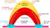 |
Fig. 14 Sketch of the scenario for energy release, transport, and conversion in solar flares. Two hot plasma components are present: one is directly heated in the corona, the other is generated by chromospheric evaporation due to energy input by nonthermal particles (particle acceleration is not considered in this sketch) and conduction. At lower and denser atmospheric layers (chromosphere and photosphere) in the loop footpoints, energy is efficiently radiated away by cooler plasma. |
Considering the results of Paper I and the present work, we can now place all this in a common framework and propose a scenario for energy release, transport, and conversion in solar flares. This scenario is sketched in Fig. 14. In Paper I, we have seen that a (super-)hot thermal plasma is generated by direct heating in the corona, which might be due to various processes associated with reconnection. At the same time, particles are accelerated to nonthermal speeds. The resulting particle beams then dump their energy into the chromosphere, where they cause chromospheric evaporation, which fills up the flaring loops with hot X-ray emitting plasma. Both the evaporated plasma and the directly heated component suffer radiative and conductive losses. The conductive losses are particularly strong and transfer energy from the hot coronal loops to the dense lower atmospheric layers at the loop footpoints (in addition to the nonthermal energy input), where the energy can be radiated away efficiently. This occurs at cooler temperatures and is therefore not detected in X-rays, but in EUV, UV, and white light. This less energetic radiation represents the bulk of the bolometric radiated energy.
The scenario presented above is consistent with both the observed bolometric losses and the thermal X-ray emission. However, the energy in nonthermal electrons is insufficient to generate and sustain the hot thermal component or to account for the total bolometric losses, in particular in the case of weaker (i.e., C-class) flares. A lower low-energy cutoff and/or the contribution of energetic ions seems to be unable to resolve this discrepancy. Thus, there has to be an additional non-beam heating mechanism. This is consistent with our conclusion from Paper I that there is a directly heated coronal plasma component. There are several potential mechanisms (see Sect. 5.7), but in addition, one point has to be stressed: no particle acceleration mechanism will be totally efficient in the sense that 100% of the free energy is converted into kinetic energy of nonthermal particles. Instead, a certain fraction of the energy will always be transferred to an enhanced Maxwellian (thermal) component. The large discrepancy between nonthermal input and heating requirements in weaker flares could imply that the acceleration mechanism works in an inefficient regime in these events, producing much plasma heating, but fewer nonthermal particles.
We are planning to continue our studies of X-ray derived flare energetics by investigating the effects of various refinements to the RHESSI spectral modeling. This will include both modifications to the thermal component (e.g., bi- or multithermal models, Kappa distributions) and modifications to the thick-target model (e.g., warm target, return current).
We refer here only to the energy released in the flare. In a solar eruptive event associated with a CME and an SEP event, additional energies have to be considered (e.g., kinetic energy of the CME). This is discussed in Emslie et al. (2012).
Acknowledgments
The work of A.W. was supported by DLR under grant No. 50 QL 0001. The authors would like to thank Matthieu Kretzschmar for insightful discussions. We are grateful to the RHESSI Team for the free access to the data and the development of the software.
References
- Akritas, M. G., & Bershady, M. A. 1996, ApJ, 470, 706 [NASA ADS] [CrossRef] [Google Scholar]
- Aschwanden, M. J. 2007, ApJ, 661, 1242 [NASA ADS] [CrossRef] [Google Scholar]
- Aschwanden, M. J., & Alexander, D. 2001, Sol. Phys., 204, 93 [NASA ADS] [CrossRef] [Google Scholar]
- Aschwanden, M. J., & Aschwanden, P. D. 2008, ApJ, 674, 544 [NASA ADS] [CrossRef] [Google Scholar]
- Aschwanden, M. J., Boerner, P., Ryan, D., et al. 2015, ApJ, 802, 53 [NASA ADS] [CrossRef] [Google Scholar]
- Aurass, H., Rausche, G., Mann, G., & Hofmann, A. 2005, A&A, 435, 1137 [NASA ADS] [CrossRef] [EDP Sciences] [Google Scholar]
- Battaglia, M., Grigis, P. C., & Benz, A. O. 2005, A&A, 439, 737 [NASA ADS] [CrossRef] [EDP Sciences] [Google Scholar]
- Battaglia, M., Fletcher, L., & Benz, A. O. 2009, A&A, 498, 891 [NASA ADS] [CrossRef] [EDP Sciences] [Google Scholar]
- Battaglia, M., Kleint, L., Krucker, S., & Graham, D. 2015, ApJ, 813, 113 [NASA ADS] [CrossRef] [Google Scholar]
- Brosius, J. W. 2013, ApJ, 762, 133 [NASA ADS] [CrossRef] [Google Scholar]
- Brosius, J. W., & Daw, A. N. 2015, ApJ, 810, 45 [NASA ADS] [CrossRef] [Google Scholar]
- Brosius, J. W., & Phillips, K. J. H. 2004, ApJ, 613, 580 [NASA ADS] [CrossRef] [Google Scholar]
- Brown, J. C. 1971, Sol. Phys., 18, 489 [NASA ADS] [CrossRef] [Google Scholar]
- Cargill, P. J., & Klimchuk, J. A. 1997, ApJ, 478, 799 [NASA ADS] [CrossRef] [Google Scholar]
- Cargill, P. J., & Priest, E. R. 1982, Sol. Phys., 76, 357 [NASA ADS] [CrossRef] [Google Scholar]
- Carmichael, H. 1964, NASA SP, 50, 451 [Google Scholar]
- Caspi, A., & Lin, R. P. 2010, ApJ, 725, L161 [NASA ADS] [CrossRef] [Google Scholar]
- Caspi, A., Krucker, S., & Lin, R. P. 2014a, ApJ, 781, 43 [NASA ADS] [CrossRef] [Google Scholar]
- Caspi, A., McTiernan, J. M., & Warren, H. P. 2014b, ApJ, 788, L31 [NASA ADS] [CrossRef] [Google Scholar]
- Czaykowska, A., De Pontieu, B., Alexander, D., & Rank, G. 1999, ApJ, 521, L75 [NASA ADS] [CrossRef] [Google Scholar]
- del Zanna, G., Berlicki, A., Schmieder, B., & Mason, H. E. 2006, Sol. Phys., 234, 95 [NASA ADS] [CrossRef] [Google Scholar]
- Dere, K. P., Landi, E., Mason, H. E., Monsignori Fossi, B. C., & Young, P. R. 1997, A&AS, 125, 149 [NASA ADS] [CrossRef] [EDP Sciences] [Google Scholar]
- Emslie, A. G., Kucharek, H., Dennis, B. R., et al. 2004, J. Geophys. Res., 109, 10104 [NASA ADS] [CrossRef] [Google Scholar]
- Emslie, A. G., Dennis, B. R., Holman, G. D., & Hudson, H. S. 2005, J. Geophys. Res., 110, 11103 [NASA ADS] [CrossRef] [Google Scholar]
- Emslie, A. G., Dennis, B. R., Shih, A. Y., et al. 2012, ApJ, 759, 71 [NASA ADS] [CrossRef] [Google Scholar]
- Fletcher, L., & Hudson, H. S. 2008, ApJ, 675, 1645 [NASA ADS] [CrossRef] [Google Scholar]
- Fletcher, L., Hannah, I. G., Hudson, H. S., & Innes, D. E. 2013, ApJ, 771, 104 [NASA ADS] [CrossRef] [Google Scholar]
- Fröhlich, C., Andersen, B. N., Appourchaux, T., et al. 1997, Sol. Phys., 170, 1 [NASA ADS] [CrossRef] [Google Scholar]
- Graham, D. R., & Cauzzi, G. 2015, ApJ, 807, L22 [NASA ADS] [CrossRef] [Google Scholar]
- Graham, D. R., Hannah, I. G., Fletcher, L., & Milligan, R. O. 2013, ApJ, 767, 83 [NASA ADS] [CrossRef] [Google Scholar]
- Grigis, P. C., & Benz, A. O. 2004, A&A, 426, 1093 [NASA ADS] [CrossRef] [EDP Sciences] [Google Scholar]
- Guo, J., Emslie, A. G., Massone, A. M., & Piana, M. 2012, ApJ, 755, 32 [NASA ADS] [CrossRef] [Google Scholar]
- Hirayama, T. 1974, Sol. Phys., 34, 323 [NASA ADS] [CrossRef] [Google Scholar]
- Holman, G. D., Sui, L., Schwartz, R. A., & Emslie, A. G. 2003, ApJ, 595, L97 [NASA ADS] [CrossRef] [Google Scholar]
- Jain, R., Awasthi, A. K., Rajpurohit, A. S., & Aschwanden, M. J. 2011, Sol. Phys., 270, 137 [NASA ADS] [CrossRef] [Google Scholar]
- Jakimiec, J., & Bąk-Stȩślicka, U. 2011, Sol. Phys., 272, 91 [NASA ADS] [CrossRef] [Google Scholar]
- Karlický, M., & Kosugi, T. 2004, A&A, 419, 1159 [NASA ADS] [CrossRef] [EDP Sciences] [Google Scholar]
- Kennedy, M. B., Milligan, R. O., Mathioudakis, M., & Keenan, F. P. 2013, ApJ, 779, 84 [NASA ADS] [CrossRef] [Google Scholar]
- Kopp, G., & Lawrence, G. 2005, Sol. Phys., 230, 91 [Google Scholar]
- Kopp, R. A., & Pneuman, G. W. 1976, Sol. Phys., 50, 85 [NASA ADS] [CrossRef] [Google Scholar]
- Kretzschmar, M. 2011, A&A, 530, A84 [NASA ADS] [CrossRef] [EDP Sciences] [Google Scholar]
- Kretzschmar, M., de Wit, T. D., Schmutz, W., et al. 2010, Nature Phys., 6, 690 [Google Scholar]
- Krucker, S., Hudson, H. S., Glesener, L., et al. 2010, ApJ, 714, 1108 [NASA ADS] [CrossRef] [Google Scholar]
- Landi, E., Young, P. R., Dere, K. P., Del Zanna, G., & Mason, H. E. 2013, ApJ, 763, 86 [NASA ADS] [CrossRef] [Google Scholar]
- Lin, R. P., Dennis, B. R., Hurford, G. J., et al. 2002, Sol. Phys., 210, 3 [Google Scholar]
- Lin, R. P., Krucker, S., Hurford, G. J., et al. 2003, ApJ, 595, L69 [NASA ADS] [CrossRef] [Google Scholar]
- Longcope, D. W., & Guidoni, S. E. 2011, ApJ, 740, 73 [NASA ADS] [CrossRef] [Google Scholar]
- Mann, G., & Warmuth, A. 2011, A&A, 528, A104 [NASA ADS] [CrossRef] [EDP Sciences] [Google Scholar]
- Mann, G., Warmuth, A., & Aurass, H. 2009, A&A, 494, 669 [NASA ADS] [CrossRef] [EDP Sciences] [Google Scholar]
- Mason, H. E., Bhatia, A. K., Neupert, W. M., Swartz, M., & Kastner, S. O. 1984, Sol. Phys., 92, 199 [NASA ADS] [CrossRef] [Google Scholar]
- Miller, J. A., Larosa, T. N., & Moore, R. L. 1996, ApJ, 461, 445 [NASA ADS] [CrossRef] [Google Scholar]
- Milligan, R. O., Gallagher, P. T., Mathioudakis, M., et al. 2006, ApJ, 638, L117 [NASA ADS] [CrossRef] [Google Scholar]
- Milligan, R. O., Kennedy, M. B., Mathioudakis, M., & Keenan, F. P. 2012, ApJ, 755, L16 [NASA ADS] [CrossRef] [Google Scholar]
- Moore, C. S., Chamberlin, P. C., & Hock, R. 2014, ApJ, 787, 32 [NASA ADS] [CrossRef] [Google Scholar]
- Neidig, D. F. 1989, Sol. Phys., 121, 261 [NASA ADS] [CrossRef] [Google Scholar]
- Neupert, W. M. 1968, ApJ, 153, L59 [NASA ADS] [CrossRef] [Google Scholar]
- Oreshina, A. V., & Oreshina, I. V. 2013, A&A, 558, A16 [NASA ADS] [CrossRef] [EDP Sciences] [Google Scholar]
- Parks, G. K., & Winckler, J. R. 1969, ApJ, 155, L117 [NASA ADS] [CrossRef] [Google Scholar]
- Petschek, H. E. 1964, NASA SP, 50, 425 [Google Scholar]
- Phillips, K. J. H., Bhatia, A. K., Mason, H. E., & Zarro, D. M. 1996, ApJ, 466, 549 [NASA ADS] [CrossRef] [Google Scholar]
- Priest, E. R. 1982, Solar Magnetohydrodynamics (Dordrecht: Reidel) [Google Scholar]
- Qiu, J., Gary, D. E., & Fleishman, G. D. 2009, Sol. Phys., 255, 107 [NASA ADS] [CrossRef] [Google Scholar]
- Rausche, G., Aurass, H., Mann, G., Karlický, M., & Vocks, C. 2007, Sol. Phys., 245, 327 [NASA ADS] [CrossRef] [Google Scholar]
- Ryan, D. F., Milligan, R. O., Gallagher, P. T., et al. 2012, ApJS, 202, 11 [NASA ADS] [CrossRef] [Google Scholar]
- Ryan, D. F., O’Flannagain, A. M., Aschwanden, M. J., & Gallagher, P. T. 2014, Sol. Phys., 289, 2547 [NASA ADS] [CrossRef] [Google Scholar]
- Sadykov, V. M., Vargas Dominguez, S., Kosovichev, A. G., et al. 2015, ApJ, 805, 167 [NASA ADS] [CrossRef] [Google Scholar]
- Saint-Hilaire, P., & Benz, A. O. 2002, Sol. Phys., 210, 287 [NASA ADS] [CrossRef] [Google Scholar]
- Saint-Hilaire, P., & Benz, A. O. 2005, A&A, 435, 743 [NASA ADS] [CrossRef] [EDP Sciences] [Google Scholar]
- Shih, A. Y., Lin, R. P., & Smith, D. M. 2009, ApJ, 698, L152 [NASA ADS] [CrossRef] [Google Scholar]
- Sturrock, P. A. 1966, Nature, 211, 695 [NASA ADS] [CrossRef] [Google Scholar]
- Sui, L., Holman, G. D., & Dennis, B. R. 2005, ApJ, 626, 1102 [NASA ADS] [CrossRef] [Google Scholar]
- Sui, L., Holman, G. D., & Dennis, B. R. 2007, ApJ, 670, 862 [NASA ADS] [CrossRef] [Google Scholar]
- Teriaca, L., Falchi, A., Cauzzi, G., et al. 2003, ApJ, 588, 596 [NASA ADS] [CrossRef] [Google Scholar]
- Veronig, A. M., Brown, J. C., Dennis, B. R., et al. 2005, ApJ, 621, 482 [Google Scholar]
- Warmuth, A., & Mann, G. 2013a, A&A, 552, A86 [NASA ADS] [CrossRef] [EDP Sciences] [Google Scholar]
- Warmuth, A., & Mann, G. 2013b, A&A, 552, A87 [NASA ADS] [CrossRef] [EDP Sciences] [Google Scholar]
- Warmuth, A., & Mann, G. 2016, A&A, 588, A115 (Paper I) [NASA ADS] [CrossRef] [EDP Sciences] [Google Scholar]
- Warmuth, A., Holman, G. D., Dennis, B. R., et al. 2009a, ApJ, 699, 917 [NASA ADS] [CrossRef] [Google Scholar]
- Warmuth, A., Mann, G., & Aurass, H. 2009b, A&A, 494, 677 [NASA ADS] [CrossRef] [EDP Sciences] [Google Scholar]
- Warren, H. P., Mariska, J. T., & Doschek, G. A. 2013, ApJ, 770, 116 [Google Scholar]
- White, S. M., Krucker, S., Shibasaki, K., et al. 2003, ApJ, 595, L111 [NASA ADS] [CrossRef] [Google Scholar]
- White, S. M., Thomas, R. J., & Schwartz, R. A. 2005, Sol. Phys., 227, 231 [NASA ADS] [CrossRef] [Google Scholar]
- Woods, T. N., Eparvier, F. G., Fontenla, J., et al. 2004, Geophys. Res. Lett., 31, L10802 [NASA ADS] [CrossRef] [Google Scholar]
- Woods, T. N., Kopp, G., & Chamberlin, P. C. 2006, JGR, 111, A10S14 [Google Scholar]
All Tables
All Figures
|
Fig. 1 Maximum thermal energies Eth derived from RHESSI (left column) and GOES (right column) as a function of the emission measure EM (top row), temperature T (2nd from top), electron density n (3rd from top), and thermal volume Vth (bottom row). We also show power-law fits obtained with the BCES bisector method (full black line). The slope α and intercept b of the obtained power law and the rank correlation coefficient R are indicated. |
| In the text | |
|
Fig. 2 Maximum radiative loss rates Prad derived from RHESSI (left column) and GOES (right column) as a function of the emission measure EM (top row), temperature T (2nd from top), electron density n (3rd from top), and thermal volume Vth (bottom row). |
| In the text | |
|
Fig. 3 Maximum conductive loss rates Pcond derived from RHESSI (left column) and GOES (right column) as a function of the emission measure EM (top row), temperature T (2nd from top), electron density n (3rd from top), and nonthermal footpoint area Anth,tot (bottom row). |
| In the text | |
|
Fig. 4 Maximum kinetic power Pnth of nonthermal electrons as a function of the electron flux Fnth (top left), nonthermal footpoint area Anth,tot (top right), low-energy cutoff EC (bottom left), and electron spectral index δL (bottom right). |
| In the text | |
|
Fig. 5 Maximum gravitational energy, Egrav (top) and maximum kinetic flow energy, Eflow (bottom) of the hot plasma plotted versus maximum thermal energy, Eth, derived from RHESSI (left) and GOES data (right). Power-law fits (full lines), the slope α and intercept b of the obtained power law, and the rank correlation coefficient R are also indicated. The dotted line denotes x = y, and the median ratio M of the different energies is indicated. Both gravitational and flow energies are significantly lower than the maximum thermal energies. |
| In the text | |
|
Fig. 6 As in Fig. 5, but showing the radiative (top) and conductive energy loss (bottom) of the hot plasma, Erad and Econd, plotted versus maximum thermal energy Eth, derived from RHESSI (left) and GOES data (right). For the radiative energy loss given by GOES, the relation derived from Emslie et al. (2012) is shown by the dash-dotted line. |
| In the text | |
|
Fig. 7 Maximum thermal energy, Eth (top), radiative loss, Erad (middle), and conductive energy loss, Econd (bottom), of the hot plasma derived from RHESSI (left) and GOES data (right), plotted versus energy input by nonthermal electrons, Enth. For Eth,G and Erad,G, the relations derived from Emslie et al. (2012) are shown by the dash-dotted line. |
| In the text | |
|
Fig. 8 Total (bolometric) radiated energies, Ebol, in solar flares as a function of peak GOES flux FG, as given by Emslie et al. (2012, diamonds) and Kretzschmar (2011, crosses). A power-law fit (dotted line) to the values of Kretzschmar (2011), its slope α and intercept b, and the rank correlation coefficient, R, are also shown. |
| In the text | |
|
Fig. 9 Maximum thermal energy, Eth (dots), as a function of the background-subtracted peak GOES flux FG, derived from RHESSI (left) and GOES data (right). We also indicate a power-law fit (full black line) of Eth , the slope α and intercept b of the obtained power law, and the rank correlation coefficient R. The corresponding relations derived by Caspi et al. (2014a) and Emslie et al. (2012) are shown as blue and red dash-dotted lines, respectively. For comparison, the total (bolometric) radiated energies, Ebol, as derived by Emslie et al. (2012, diamonds) and Kretzschmar (2011, crosses), are also shown. The dotted green line shows a power law fitted to Ebol as derived by Kretzschmar (2011). |
| In the text | |
|
Fig. 10 As in Fig. 9, but showing the radiative energy loss, Erad (dots), as a function of peak GOES flux FG, derived from RHESSI (left) and GOES data (right). The corresponding relations derived by Ryan et al. (2012) and Emslie et al. (2012) are shown as orange and red dash-dotted lines, respectively. |
| In the text | |
|
Fig. 11 As in Fig. 9, but showing the conductive energy loss, Econd (dots), as a function of peak GOES flux FG, derived from RHESSI (left) and GOES data (right). |
| In the text | |
|
Fig. 12 As in Fig. 9, but showing the total injected energy in nonthermal electrons, Enth (dots), as a function of peak GOES flux FG. The red dash-dotted line indicates the relation derived by Emslie et al. (2012). |
| In the text | |
|
Fig. 13 As in Fig. 9, but showing the total energy required for heating the hot thermal plasma, Eh (red dots), as a function of peak GOES flux FG. For comparison, the energy in nonthermal electrons Enth (blue dots) and the total radiated energy Ebol (green crosses and diamonds) is shown. |
| In the text | |
|
Fig. 14 Sketch of the scenario for energy release, transport, and conversion in solar flares. Two hot plasma components are present: one is directly heated in the corona, the other is generated by chromospheric evaporation due to energy input by nonthermal particles (particle acceleration is not considered in this sketch) and conduction. At lower and denser atmospheric layers (chromosphere and photosphere) in the loop footpoints, energy is efficiently radiated away by cooler plasma. |
| In the text | |
Current usage metrics show cumulative count of Article Views (full-text article views including HTML views, PDF and ePub downloads, according to the available data) and Abstracts Views on Vision4Press platform.
Data correspond to usage on the plateform after 2015. The current usage metrics is available 48-96 hours after online publication and is updated daily on week days.
Initial download of the metrics may take a while.