| Issue |
A&A
Volume 588, April 2016
|
|
|---|---|---|
| Article Number | A93 | |
| Number of page(s) | 12 | |
| Section | Extragalactic astronomy | |
| DOI | https://doi.org/10.1051/0004-6361/201527398 | |
| Published online | 23 March 2016 | |
New quasars behind the Magellanic Clouds. Spectroscopic confirmation of near-infrared selected candidates
1
European Southern Observatory, Ave. Alonso de Córdova 3107, Vitacura,
Santiago,
Chile
e-mail:
This email address is being protected from spambots. You need JavaScript enabled to view it.
2
European Southern Observatory, Karl-Schwarzschild-Str. 2, 85748
Garching bei München,
Germany
3
Universität Potsdam, Institut für Physik und
Astronomie, Karl-Liebknecht-Str.
24/25, 14476
Potsdam,
Germany
4
Leibniz-Institut für Astrophysik Potsdam,
An der Sternwarte 16,
14482
Potsdam,
Germany
5
University of Hertfordshire, Physics Astronomy and Mathematics, College Lane,
Hatfield
AL10 9AB,
UK
6
ICRAR, M468, The University of Western Australia,
35 Stirling Hwy, 6009 Crawley,
Western Australia,
Australia
7
Kavli Institute for Astronomy and Astrophysics, Peking
University, Yi He Yuan Lu 5, Hai
Dian District, 100871
Beijing, PR
China
8
Department of Astronomy, Peking University,
Yi He Yuan Lu 5, Hai Dian District,
100871
Beijing, PR
China
9
International Space Science Institute-Beijing,
1 Nanertiao, Hai Dian District,
100190
Beijing, PR
China
10
School of Physics and Astronomy, Queen Mary University of
London, Mile End
Road, London
E1 4NS,
UK
11
E.A. Milne Centre for Astrophysics, Department of Physics
& Mathematics, University of Hull, Hull
HU6 7RX,
UK
12
Instituut voor Sterrenkunde, K. U. Leuven, Celestijnenlaan 200D
bus 2401, 3001
Leuven,
Belgium
13
Lennard-Jones Laboratories, Keele University,
ST5 5BG, UK
14
Observatorio Astronómico, Universidad Nacional de
Córdoba, Laprida
854, 5000
Córdoba,
Argentina
15
Consejo Nacional de Investigaciones Científicas y Técnicas, Av.
Rivadavia 1917, C1033AAJ, Buenos
Aires, Argentina
Received: 18 September 2015
Accepted: 19 October 2015
Abstract
Context. Quasi-stellar objects (quasars) located behind nearby galaxies provide an excellent absolute reference system for astrometric studies, but they are difficult to identify because of fore- and background contamination. Deep wide-field, high angular resolution surveys spanning the entire area of nearby galaxies are needed to obtain a complete census of such quasars.
Aims. We embarked on a program to expand the quasar reference system behind the Large and the Small Magellanic Clouds, the Magellanic Bridge, and the Magellanic Stream that connects the Clouds with the Milky Way.
Methods. Hundreds of quasar candidates were selected based on their near-infrared colors and variability properties from the ongoing public ESO VISTA Magellanic Clouds survey. A subset of 49 objects was followed up with optical spectroscopy.
Results. We confirmed the quasar nature of 37 objects (34 new identifications): four are low redshift objects, three are probably stars, and the remaining three lack prominent spectral features for a secure classification. The bona fide quasars, identified from their broad emisison lines, are located as follows: 10 behind the LMC, 13 behind the SMC, and 14 behind the Bridge. The quasars span a redshift range from z ~ 0.5 to z ~ 4.1.
Conclusions. Upon completion the VMC survey is expected to yield a total of ~1500 quasars with Y< 19.32 mag, J< 19.09 mag, and Ks< 18.04 mag.
Key words: surveys / infrared: galaxies / quasars: general / Magellanic Clouds
© ESO, 2016
1. Introduction
Quasi–stellar objects (quasars) are active nuclei of distant galaxies undergoing episodes of strong accretion. Typically, the contribution from the host galaxy is negligible and they appear as point-like objects with strong emission lines. Quasar candidates are often identified by their variability, a method pioneered by Hook et al. (1994). The recent studies of Gallastegui-Aizpun & Sarajedini (2014), Cartier et al. (2015), and Peters et al. (2015), among others, brought the number of sampled objects up to many thousands. Precise space-based photometry was also used (the Kepler mission; Shaya et al. 2015). Gregg et al. (1996) reported a large quasar selection based on their radio properties (see also White et al. 2000; Becker et al. 2001). The radio selection has often been complemented with other wavelength regimes to sample dusty reddened objects (Glikman et al. 2012). Shanks et al. (1991) demonstrated that the quasars contribute at least a third of the X-ray sky background. The realization that they are powerful X-ray sources led to identification of a large number of faint quasars (e.g., Boyle et al. 1993; Hasinger et al. 1998, and the subsequent papers in these series). Modern X-ray missions continue to contribute to this field (Loaring et al. 2005; Nandra et al. 2005). More recently, the distinct mid–infrared properties of quasars have come to attention, mainly due to the work of Lacy et al. (2004). These properties have been exploited further by Stern et al. (2012), Assef et al. (2013), and Ross et al. (2015). Finally, multi-wavelength selections are becoming common (DiPompeo et al. 2015).
Quasars are easily confirmed from optical spectroscopy, aiming to detect broad hydrogen (Lyα 1216 Å, Hδ 4101 Å, Hγ 4340 Å, Hβ 4861 Å, Hα 6563 Å), magnesium (Mgii 2800 Å), and carbon (Civ 1549 Å, Ciii] 1909 Å) lines, as well as some narrow forbidden lines of oxygen ([Oii] 3727 Å, [Oiii] 4959 Å, 5007 Å). These lines also help to derive the quasars’ redshifts (e.g., Vanden Berk et al. 2001).
Quasars are cosmological probes and serve as background “lights” to explore the intervening interstellar medium, but they also are distant unmoving objects used to establish an absolute astrometric reference system on the sky. The smaller the measured proper motions (PMs) of foreground objects are, the more useful the quasars become – as is the case for nearby galaxies. Quasars behind these galaxies are hard to identify because of foreground contamination, the additional reddening inside the galaxies themselves (owing to dust), and the galaxies relatively large angular areas on the sky, which implies the need to carry out dedicated wide-field surveys, sometimes covering hundreds of square degrees. The Magellanic Clouds system is an extreme case where these obstacles are notably enhanced: the combined area of the two galaxies, the Magellanic Bridge, and the Stream that connects them with the Milky Way is at least two hundred square degrees; the significant depth of the Small Magellanic Cloud (SMC) along the line of sight (e.g., de Grijs & Bono 2015) aggravates the contamination and reddening issues.
Cioni et al. (2013) reviewed previous works aiming at discovering quasars behind the Magellanic Clouds: Blanco & Heathcote (1986), Dobrzycki et al. (2002, 2003b,a, 2005), Geha et al. (2003), Kozłowski & Kochanek (2009), Kozłowski et al. (2012, 2011), and Véron-Cetty & Véron (2010). In this study we add the latest installment of the Magellanic Quasar Survey (MQS) by Kozłowski et al. (2013), who increased the number of spectroscopically confirmed quasars behind the Large Magellanic Cloud (LMC) and SMC to 758, almost an order of a magnitude higher than before.
The optical surveys can easily miss or misclassify some quasars; near- and mid-infrared surveys are necessary to obtain more complete samples; ~90% of the MQS quasar candidates were selected from mid-IR Spitzer observations (see also van Loon & Sansom 2015). This motivated us to search for quasars in the VISTA (Visual and Infrared Survey Telescope for Astronomy; Emerson et al. 2006) Survey of the Magellanic Clouds system (VMC; Cioni et al. 2011). The European Southern Observatory’s (ESO) VISTA is a 4.1 m telescope located on Cerro Paranal; it is equipped with VIRCAM (VISTA InfraRed CAMera; Dalton et al. 2006), a wide-field near-infrared camera producing ~1 × 1.5 deg2 tiles1 working in the 0.9–2.4 μm wavelength range. The VISTA data are processed with the VISTA Data Flow System (VDFS; Irwin et al. 2004; Emerson et al. 2004) pipeline at the Cambridge Astronomical Survey Unit2. The data products are available through the ESO archive or the specialized VISTA Science Archive (VSA; Cross et al. 2012).
The VMC is an ESO public survey, covering 184 deg2 around the LMC, SMC, and the Magellanic Bridge and Stream, down to Ks = 20.3 mag (S/N ~ 10; Vega system) in three epochs in the Y and J-bands, and 12 epochs in the Ks-band, spread over at least a year. The main survey goal is to study the star formation history (Kerber et al. 2009; Rubele et al. 2012, 2015; Tatton et al. 2013) and the geometry (Ripepi et al. 2012a,b, 2014, 2015; Tatton et al. 2013; Moretti et al. 2014; Muraveva et al. 2014) of the system. Furthermore, the depth and angular resolution of the VMC survey has the potential to enable detailed studies of the star and cluster populations (Miszalski et al. 2011; Gullieuszik et al. 2012; Li et al. 2014; Piatti et al. 2014, 2015b,a), including PM measurements.
Cioni et al. (2014) measured the PM of the LMC from one ~1.5 deg2 tile, comparing the VISTA and 2MASS (Two Micron All Sky Survey; Skrutskie et al. 2003) data over a time baseline of about ten years and from VMC data alone within a time span of ~1 yr. They used ~40 000 stellar positions and a reference system established by ~8000 background galaxies. Similarly, Cioni et al. (2015), measured the PM of the SMC with respect to ~20 000 background galaxies. Background galaxies are numerous, but they are extended sources, and their positions cannot be measured as accurately as the positions of point sources. This motivated us to persist with our search and confirmation of background quasars. The current paper reports spectroscopic follow-up observations of the VMC quasar candidates from a pilot study of only 7 out of the 110 VMC tiles, which were the only ones completely observed at the time of the search. The full-scale project intends to select for the first time quasar candidates in the near-infrared over the entire Magellanic system.
VMC quasar parameters (in order of increasing right ascension).
2. Sample selection
Cioni et al. (2013) derived selection criteria to identify candidate quasars based on the locus of 117 known quasars in a (Y−J) versus (J−Ks) color–color diagram, and their Ks-band variability behavior. The diagram was based on average magnitudes obtained from deep tile images created by the Wide Field Astronomy Unit (WFAU3) as part of the VMC data processing with version 1.3.0 of the VDFS pipeline. The sample selected for our study is based on these criteria and we refer the reader to Cioni et al. (2013) for details. Table 1 lists the VMC identification (Col. 1), right ascension α and declination δ (J2000; Cols. 2 and 3), magnitudes in the Y, J, and Ks-bands (Cols. 4, 6, and 8), respectively, and their associated photometric uncertainties (Cols. 5, 7, and 9) for each candidate, while Col. 10 shows the object identification (ID) used in the spectroscopic observations4. The last is composed of two parts: the first indicating the VMC tile and the second representing the sequential number of the object in the catalog of all sources in that tile; the letter g indicates that a source was classified as extended by the VDFS pipeline. Extended sources were included in our search to ensure that low redshift quasars with considerable contribution from the host galaxy will not be omitted. Their extended nature is marginal because they are dominated by the nuclei and because they are still useful for quasar absorption line studies.
The sixty-eight brightest candidates were selected to homogeneously sample seven VMC tiles where quasars had not yet been found. The total number of candidates can increase greatly if fainter objects are considered. Forty-nine of these were followed up spectroscopically. Some contamination from young stellar objects, brown dwarfs, planetary nebulae, and post-AGB stars is expected. Cioni et al. (2013) estimated that the total number of quasars with Y< 19.32 mag, J< 19.09 mag, and Ks< 18.04 mag is 1200 behind the LMC, 400 behind the SMC, 200 behind the Bridge, and 30 behind the Stream. Figure 1 shows the location of all confirmed quasars from the MQS and our candidates selected for follow-up spectroscopy in the (Y−J) versus (J−Ks) color–color diagram. A sky map showing our program objects is shown in Fig. 2, while Fig. A.1 depicts Y-band finding charts for all candidates. Most of our candidates are located in a sky area external to the OGLE III area studied by Kozłowski et al. (2013).
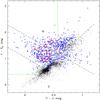 |
Fig. 1 Color–color diagram demonstrating the color selection of quasar candidates. The dashed black lines identify the regions (labeled with letters) where known quasars are found, while the green line marks the blue border of the planetary nebulae locus (Cioni et al. 2013). Our spectroscopically followed up quasars are marked with solid red dots, the non–quasars are marked with red triangles. Blue ×’s indicate the location of the VMC counterparts to the spectroscopically confirmed quasars from Kozłowski et al. (2013), selected adopting a maximum matching radius of 1 arcsec (the average separation is 0.15 ± 0.26 arcsec). Black dots are randomly drawn LMC objects (with errors in all three bands <0.1 mag) to demonstrate the locus of “normal” stars. Contaminating background galaxies are included among the black dots in regions B and C. |
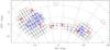 |
Fig. 2 Location of the spectroscopically followed up quasar candidates in this work (red) and confirmed quasars from Kozłowski et al. (2013) (blue). The VMC tiles are shown as contiguous rectangles. The dashed grid shows lines of constant right ascension (spaced by 15°) and constant declination (spaced by 5°). Coordinates are given with respect to (α0, δ0) = (51°, −69°). |
Derived parameters for the object in this paper.
3. Spectroscopic follow-up observations
Follow-up spectra of 49 candidates were obtained with the FOcal Reducer and low dispersion Spectrograph (FORS2; Appenzeller et al. 1998) on the Very Large Telescope (VLT) in September−November 2013 in long-slit mode with the 300V+10 grism, GG435+81 order sorting filter, and 1.3 arcsec wide slit delivering spectra over λλ = 445–865 nm with a spectral resolving power R = λ/Δλ ~ 440. Two 450 s exposures were taken for most objects, except for some cases when the exposure time was 900 s. Occasionally, spectra were repeated because the weather deteriorated during the observations. We used some of the poor quality data, and a few objects objects ended up with more than two spectra. The signal-to-noise ratio varies across the spectra, but typically it is ~10–30 at λ ~ 6000–6200 Å. The observing details, including starting times, exposure times, starting and ending airmasses, and slit position angles for each exposure are listed in Table A.1. The reduced spectra are shown in Fig. 3.
The data reduction was carried out with the ESO pipeline, version 5.0.0. The spectrophotometric calibration was carried out with spectrophotometric standards (Oke 1990; Hamuy et al. 1992, 1994; Moehler et al. 2014a,b), observed and processed in the same manner as the program spectra. Various IRAF5 tasks from the onedspec and rv packages were used in the subsequent analysis.
Quasar redshifts were measured in two steps. First, we visually identified the emission lines by comparing our spectra with the SDSS quasar composite spectrum (Vanden Berk et al. 2001). Given our wavelength coverage, if only one feature is visible, it is most likely Mgii at z ~ 1.1–1.3, otherwise another of the more prominent quasar lines would have to fall within the observed spectral range. Then, we measured the wavelengths of the features (mostly emission lines, but also some hydrogen absorption lines visible in the lower redshift objects), fitting them with a Gaussian profile using the IRAF task splot. This proved to be an adequate representation given the low resolution of our spectra. The lines, their observed wavelengths, and the derived redshifts are listed in Table A.1. Some emission lines were omitted if they fell near the edge of the wavelength range or if they were contaminated by sky emission lines and the sky subtraction left significant residuals. For most line centers the typical formal statistical errors are ~1 Å and they translate into redshift errors of less than 0.001. These are optimistic estimates that neglect the wavelength calibration error. We evaluated these errors by measuring the wavelengths of 45 strong and isolated sky lines in five randomly selected spectra from our sample; we found no trends with wavelength and an rms of 1.57 Å. This translates into a redshift uncertainty of ~0.0002 for a line at 7000 Å near the center of our spectral coverage.
To evaluate the real uncertainties we compared the redshifts derived from different lines of the same object (Fig. 4, top). The average difference for 35 pairs of lines is approximately zero: ⟨|zi−zj|⟩ = 0.006 ± 0.007. For objects with multiple lines we adopted the average difference as redshift error, adding in quadrature the wavelength calibration error of 0.0002. This addition only made a difference for a few low redshift objects. For quasars for which only a single line was available, we conservatively adopted a redshift error value of 0.005 for objects with z< 1 and 0.015 for the more distant ones. Finally, as external verification we re–measured in the rest–frame SDSS composite spectrum the redshifts of the same lines that were detected in our spectra, obtaining values below 0.0001, as expected.
 |
Fig. 3 Spectra of the quasar candidates sorted by redshift and shifted to rest-frame wavelength. The spectra were normalized to an average value of one and shifted vertically by offsets of two, four, etc., for display purposes. The SDSS composite quasar spectrum (Vanden Berk et al. 2001) is shown at the top of all panels. A sky spectrum is shown at the bottom of the fifth panel (see the next page). Objects with no measured redshift due to lack of lines or low signal-to-noise are plotted assuming z = 0 in the fifth panel next to the sky spectrum to facilitate the identification of the residuals from the sky emission lines. |
4. Results
The majority of the observed objects are quasars: 37 objects (in the first four panels of Fig. 3) appear to be bona fide quasars at z ~ 0.47–4.10; they show some broad emission lines even though some spectra need smoothing (block averaging, typically by 4−8 resolution bins) for display purposes. The spectra of the three highest redshift quasars show Lyα absorption systems; a few quasars (e.g., SMC 3_5 22, BRI 2_8 197, etc.) show blueshifted Civ absorption (Fig. 3, panel 1), perhaps due to an AGN wind. We defer more detailed study of individual objects until the rest of the sample has been followed up.
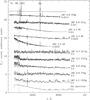 |
Fig. 3 continued. |
These objects are marked in the last column of Table A.1 as quasars: 10 are behind the LMC, 13 behind the SMC, and 14 behind the Bridge area. The VDFS pipeline classified 28 of the confirmed quasars as point sources and 9 as extended (recognizable by the “g” in their names). This does not necessarily mean that the VISTA data resolved their host galaxies since the extended sources are uniformly spread over the redshift range – about half of them have z ~ 1–2 – and random alignment with objects in the Magellanic Clouds can easily affect their appearance. Our success rate is ~76%, testifying to the robustness and reliability of our selection criteria. There are more candidates that turned out not to be quasars in region B than in region A of the color–color diagram (see Fig. 1), but for now our statistical basis is small; a follow up of more candidates is needed to draw any definitive conclusion.
The majority of quasars with redshift z ≤ 1 were classified as extended sources by the VDFS pipeline, supporting our decision to include extended objects in the sample. Four extended objects are contaminating low redshift galaxies: LMC 9_3 2728g, LMC 8_8 655g, and LMC 8_8 208g show hydrogen, some oxygen, and nitrogen in emission, but no obvious broad lines, so we interpret these as indicators of ongoing star formation rather than nuclear activity, while LMC 8_8 341g may also show Hβ in absorption. Furthermore, LMC 8_8 341g has a recession velocity of ~300 km s-1, consistent within the uncertainties with LMC membership (Vrad = 262.2 ± 3.4 km s-1, McConnachie 2012), which makes it a possible moderately young LMC cluster. The spectra of all these objects are shown in Fig. 3, panel 5.
Three point–source–like objects are most likely emission line stars: LMC 4_3 95, LMC 4_3 86, and SMC 3_5 29. These spectra are also shown in Fig. 3, panel 5.
The spectra of LMC 8_8 422g, LMC 4_3 3314g, and LMC 9_3 3107g (Fig. 3, panel 5) offer no solid clues as to their nature. Some BL Lacertae – active galaxies believed to be seen along a relativistic jet coming out of the nucleus – are also featureless, but they usually have bluer continua than the spectra of these three objects (Landoni et al. 2013)6. A possible test is to search for rapid variability, typical of BL Lacs, but the VMC cadence is not well suited for such an exercise, and the light curves of the three objects show no peculiarities. Finally, the spectra of LMC 4_3 1029g and LMC 8_8 376g (Fig. 3, panel 5) are too noisy for secure classification. The spectra of the five objects with no classification are plotted in the last panel in Fig. 3 at redshifts z = 0 to facilitate easier comparison with the sky spectrum shown just below them.
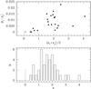 |
Fig. 4 Top: differences between redshifts zi and zj derived from each available pair of lines i and j for objects with multiple lines for bona fide quasars (solid dots) and galaxies (circles). Bottom: redshift histogram for 47 objects in our sample with reliably detected emission lines for bona fide quasars (solid line) and galaxies (dashed line). |
After target selection we realized that three of our candidates were previously confirmed quasars, and two more were suspected to be quasars. Tinney et al. (1997) selected SMC 5_2 203 (their designation [TDZ97] QJ0035−7201 or SMC-X1-R-4; our spectrum is plotted in Fig. 3, panel 4) from unpublished ROSAT SMC observations. They confirmed it spectroscopically and estimated a redshift of z = 0.666 ± 0.001, in excellent agreement with our value of z = 0.667 ± 0.015. Kozłowski et al. (2013) identified SMC 3_5 24 and SMC 3_5 15 (Fig. 3, panels 2 and 3, respectively) and reported spectroscopic confirmation of their quasar nature, measuring redshifts of z = 1.820 and z = 1.549, respectively, also very similar to our values of z = 1.821 ± 0.013 and z = 1.543 ± 0.015. LMC 9_3 137 and LMC 4_3 95g were listed as AGN candidates by Kozłowski & Kochanek (2009): [KK2009] J050434.46−641844.4 and [KK2009] J045709.93−713231.0 based on their mid-infrared colors (Fig. 3, panels 2 and 3, respectively).
The ROSAT all-sky survey (Voges et al. 1999) reported an X-ray source at a separation of 7″ from our estimated position of the confirmed quasar LMC 8_8 119 (Fig. 3, panel 4). Flesch (2010) associated the X-ray source with a faint object on the Palomar Observatory Sky Survey, but estimated 50% probability that this is a random alignment, and only 17% that the X-ray emission originates from a quasar.
Many of our quasars are present in the GALEX (Galaxy Evolution Explorer; Morrissey et al. 2007) source catalog, and in the SAGE–SMC (Surveying the Agents of Galaxy Evolution – Small Magellanic Cloud; Gordon et al. 2011) source catalog. The confirmed quasar SMC 5_2 241 (Fig. 3, panel 1) stands out; in addition to the GALEX and SAGE detections, it has a candidate radio counterpart: SUMSS J002956−714640 at 2.8 arcsec separation from the 843 MHz Sydney University Molonglo Sky Survey (Bock et al. 1999; Mauch et al. 2003).
We revised the light curves of our observed objects because a larger number of Ks-band measurements have become available since the target selection in Cioni et al. (2013), allowing us to investigate further the near-infrared variability properties of the quasars. Light curves based on all individual pawprint measurements from all processed data at CASU as of March 2015 for all our objects are shown in Fig. A.2. We applied the same variability parameterization with the slope of a linear fit to the light curve, as in Cioni et al. (2013). The distribution of absolute slope values (i.e., slope variation) shows a dip corresponding to flat light curves, which corresponds to our criterion to select variable sources with slope variation >0.0001 mag day-1 (Fig. 5). The additional data have moved some of the selected quasars into the low-variation zone.
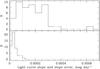 |
Fig. 5 Histograms of the slope variations (top; the vertical dashed line shows the slope variation limit of 0.0001 mag day-1, adopted in our quasar selection) and the slope uncertainties (bottom) for linear fits to the light curves of the objects in our sample. |
Cioni et al. (2013) estimated that the VMC survey will find in total about 1830 quasars. The success rate of 76% reached in this paper brings this number down to about 1390. The spectra of the candidates in 7 tiles out of the 110 tiles that comprise the entire VMC survey yielded on average ~5.3 quasars per tile. Scaling this number up to the full survey area yields ~580 quasars. This is a lower limit because only the brightest candidates in the seven tiles were followed up, so the larger number is still a viable prediction.
5. Summary
We report spectroscopic follow-up observations of 49 quasar candidates selected based on their colors and variability. They are located behind the LMC, SMC, and the Bridge area connecting the Clouds: 37 of these objects are bona fide quasars of which 34 are new discoveries. Therefore, the success rate of our quasar search is ~76%. The project is still at an early stage, but once the spectroscopic confirmation has been obtained, the identified quasars will provide an excellent reference system for detailed astrometric studies of the Magellanic Cloud system. Furthermore, the homogeneous multi-epoch observations of the VMC survey, together with the large quasar sample, open up the possibility of investigating in detail the mechanisms that drive quasar variability, for example, with structure functions in the near-infrared, following the example of the SDSS quasar variability studies (e.g., Vanden Berk et al. 2004).
Tiles are contiguous images that combine six pawprints taken in an offset pattern; pawprint is an individual VIRCAM pointing that generates a non-contiguous image of the sky because of the gaps between the 16 detectors. See Cioni et al. (2011) for details on the VMC observing strategy.
For the ESO Science Archive users: in the headers of the raw data LMC 4_3 2050g was mislabeled as LMC 4_3 2450g.
The Image Reduction and Analysis Facility is distributed by the National Optical Astronomy Observatory, which is operated by the Association of Universities for Research in Astronomy (AURA) under a cooperative agreement with the National Science Foundation.
Spectral library: http://archive.oapd.inaf.it/zbllac/
Acknowledgments
This paper is based on observations made with ESO telescopes at the La Silla Paranal Observatory under program ID 092.B-0104(A). We have made extensive use of the SIMBAD Database at CDS (Centre de Données astronomiques) Strasbourg, the NASA/IPAC Extragalactic Database (NED) which is operated by the Jet Propulsion Laboratory, CalTech, under contract with NASA, and of the VizieR catalog access tool, CDS, Strasbourg, France. R.d.G. acknowledges funding from the National Natural Science Foundation of China (grant 11373010). We thank the anonymous referee for the comments that helped to improve the paper.
References
- Appenzeller, I., Fricke, K., Fürtig, W., et al. 1998, The Messenger, 94, 1 [NASA ADS] [Google Scholar]
- Assef, R. J., Stern, D., Kochanek, C. S., et al. 2013, ApJ, 772, 26 [NASA ADS] [CrossRef] [Google Scholar]
- Becker, R. H., White, R. L., Gregg, M. D., et al. 2001, ApJS, 135, 227 [NASA ADS] [CrossRef] [Google Scholar]
- Blanco, V. M., & Heathcote, S. 1986, PASP, 98, 635 [NASA ADS] [CrossRef] [Google Scholar]
- Bock, D. C.-J., Large, M. I., & Sadler, E. M. 1999, AJ, 117, 1578 [NASA ADS] [CrossRef] [Google Scholar]
- Boyle, B. J., Griffiths, R. E., Shanks, T., Stewart, G. C., & Georgantopoulos, I. 1993, MNRAS, 260, 49 [NASA ADS] [CrossRef] [Google Scholar]
- Cartier, R., Lira, P., Coppi, P., et al. 2015, ApJ, 810, 164 [NASA ADS] [CrossRef] [Google Scholar]
- Cioni, M.-R. L., Clementini, G., Girardi, L., et al. 2011, A&A, 527, A116 [NASA ADS] [CrossRef] [EDP Sciences] [Google Scholar]
- Cioni, M.-R. L., Kamath, D., Rubele, S., et al. 2013, A&A, 549, A29 [NASA ADS] [CrossRef] [EDP Sciences] [Google Scholar]
- Cioni, M.-R. L., Girardi, L., Moretti, M. I., et al. 2014, A&A, 562, A32 [NASA ADS] [CrossRef] [EDP Sciences] [Google Scholar]
- Cioni, M.-R. L., Bekki, K., Girardi, L., et al. 2015, ArXiv e-prints [arXiv:1510.07647] [Google Scholar]
- Cross, N. J. G., Collins, R. S., Mann, R. G., et al. 2012, A&A, 548, A119 [NASA ADS] [CrossRef] [EDP Sciences] [Google Scholar]
- Dalton, G. B., Caldwell, M., Ward, A. K., et al. 2006, in SPIE Conf. Ser., 6269, 30 [Google Scholar]
- de Grijs, R., & Bono, G. 2015, AJ, 149, 179 [NASA ADS] [CrossRef] [Google Scholar]
- DiPompeo, M. A., Bovy, J., Myers, A. D., & Lang, D. 2015, MNRAS, 452, 3124 [NASA ADS] [CrossRef] [Google Scholar]
- Dobrzycki, A., Groot, P. J., Macri, L. M., & Stanek, K. Z. 2002, ApJ, 569, L15 [NASA ADS] [CrossRef] [Google Scholar]
- Dobrzycki, A., Macri, L. M., Stanek, K. Z., & Groot, P. J. 2003a, AJ, 125, 1330 [NASA ADS] [CrossRef] [Google Scholar]
- Dobrzycki, A., Stanek, K. Z., Macri, L. M., & Groot, P. J. 2003b, AJ, 126, 734 [NASA ADS] [CrossRef] [Google Scholar]
- Dobrzycki, A., Eyer, L., Stanek, K. Z., & Macri, L. M. 2005, A&A, 442, 495 [NASA ADS] [CrossRef] [EDP Sciences] [Google Scholar]
- Emerson, J. P., Irwin, M. J., Lewis, J., et al. 2004, in SPIE Conf. Ser., 5493, 401 [Google Scholar]
- Emerson, J., McPherson, A., & Sutherland, W. 2006, The Messenger, 126, 41 [NASA ADS] [Google Scholar]
- Flesch, E. 2010, PASA, 27, 283 [NASA ADS] [CrossRef] [Google Scholar]
- Gallastegui-Aizpun, U., & Sarajedini, V. L. 2014, MNRAS, 444, 3078 [NASA ADS] [CrossRef] [Google Scholar]
- Geha, M., Alcock, C., Allsman, R. A., et al. 2003, AJ, 125, 1 [NASA ADS] [CrossRef] [Google Scholar]
- Glikman, E., Urrutia, T., Lacy, M., et al. 2012, ApJ, 757, 51 [NASA ADS] [CrossRef] [Google Scholar]
- Gordon, K. D., Meixner, M., Meade, M. R., et al. 2011, AJ, 142, 102 [NASA ADS] [CrossRef] [Google Scholar]
- Gregg, M. D., Becker, R. H., White, R. L., et al. 1996, AJ, 112, 407 [NASA ADS] [CrossRef] [Google Scholar]
- Gullieuszik, M., Groenewegen, M. A. T., Cioni, M.-R. L., et al. 2012, A&A, 537, A105 [NASA ADS] [CrossRef] [EDP Sciences] [Google Scholar]
- Hamuy, M., Walker, A. R., Suntzeff, N. B., et al. 1992, PASP, 104, 533 [NASA ADS] [CrossRef] [Google Scholar]
- Hamuy, M., Suntzeff, N. B., Heathcote, S. R., et al. 1994, PASP, 106, 566 [NASA ADS] [CrossRef] [Google Scholar]
- Hasinger, G., Burg, R., Giacconi, R., et al. 1998, A&A, 329, 482 [NASA ADS] [Google Scholar]
- Hook, I. M., McMahon, R. G., Boyle, B. J., & Irwin, M. J. 1994, MNRAS, 268, 305 [NASA ADS] [CrossRef] [Google Scholar]
- Irwin, M. J., Lewis, J., Hodgkin, S., et al. 2004, in SPIE Conf. Ser., 5493, 411 [Google Scholar]
- Kerber, L. O., Girardi, L., Rubele, S., & Cioni, M.-R. 2009, A&A, 499, 697 [NASA ADS] [CrossRef] [EDP Sciences] [Google Scholar]
- Kozłowski, S., & Kochanek, C. S. 2009, ApJ, 701, 508 [NASA ADS] [CrossRef] [Google Scholar]
- Kozłowski, S., Kochanek, C. S., & Udalski, A. 2011, ApJS, 194, 22 [NASA ADS] [CrossRef] [Google Scholar]
- Kozłowski, S., Kochanek, C. S., Jacyszyn, A. M., et al. 2012, ApJ, 746, 27 [NASA ADS] [CrossRef] [Google Scholar]
- Kozłowski, S., Onken, C. A., Kochanek, C. S., et al. 2013, ApJ, 775, 92 [NASA ADS] [CrossRef] [Google Scholar]
- Lacy, M., Storrie-Lombardi, L. J., Sajina, A., et al. 2004, ApJS, 154, 166 [NASA ADS] [CrossRef] [Google Scholar]
- Landoni, M., Falomo, R., Treves, A., et al. 2013, AJ, 145, 114 [NASA ADS] [CrossRef] [Google Scholar]
- Li, C., de Grijs, R., Deng, L., et al. 2014, ApJ, 790, 35 [NASA ADS] [CrossRef] [Google Scholar]
- Loaring, N. S., Dwelly, T., Page, M. J., et al. 2005, MNRAS, 362, 1371 [NASA ADS] [CrossRef] [Google Scholar]
- Mauch, T., Murphy, T., Buttery, H. J., et al. 2003, MNRAS, 342, 1117 [NASA ADS] [CrossRef] [Google Scholar]
- McConnachie, A. W. 2012, AJ, 144, 4 [NASA ADS] [CrossRef] [Google Scholar]
- Miszalski, B., Napiwotzki, R., Cioni, M.-R. L., et al. 2011, A&A, 531, A157 [NASA ADS] [CrossRef] [EDP Sciences] [Google Scholar]
- Moehler, S., Modigliani, A., Freudling, W., et al. 2014a, The Messenger, 158, 16 [NASA ADS] [Google Scholar]
- Moehler, S., Modigliani, A., Freudling, W., et al. 2014b, A&A, 568, A9 [NASA ADS] [CrossRef] [EDP Sciences] [Google Scholar]
- Moretti, M. I., Clementini, G., Muraveva, T., et al. 2014, MNRAS, 437, 2702 [NASA ADS] [CrossRef] [Google Scholar]
- Morrissey, P., Conrow, T., Barlow, T. A., et al. 2007, ApJS, 173, 682 [NASA ADS] [CrossRef] [Google Scholar]
- Muraveva, T., Clementini, G., Maceroni, C., et al. 2014, MNRAS, 443, 432 [NASA ADS] [CrossRef] [Google Scholar]
- Nandra, K., Laird, E. S., Adelberger, K., et al. 2005, MNRAS, 356, 568 [NASA ADS] [CrossRef] [Google Scholar]
- Oke, J. B. 1990, AJ, 99, 1621 [NASA ADS] [CrossRef] [Google Scholar]
- Peters, C. M., Richards, G. T., Myers, A. D., et al. 2015, ApJ, 811, 95 [NASA ADS] [CrossRef] [Google Scholar]
- Piatti, A. E., Guandalini, R., Ivanov, V. D., et al. 2014, A&A, 570, A74 [NASA ADS] [CrossRef] [EDP Sciences] [Google Scholar]
- Piatti, A. E., de Grijs, R., Ripepi, V., et al. 2015a, MNRAS, 454, 839 [NASA ADS] [CrossRef] [Google Scholar]
- Piatti, A. E., de Grijs, R., Rubele, S., et al. 2015b, MNRAS, 450, 552 [NASA ADS] [CrossRef] [Google Scholar]
- Ripepi, V., Moretti, M. I., Clementini, G., et al. 2012a, Ap&SS, 341, 51 [NASA ADS] [CrossRef] [Google Scholar]
- Ripepi, V., Moretti, M. I., Marconi, M., et al. 2012b, MNRAS, 424, 1807 [NASA ADS] [CrossRef] [Google Scholar]
- Ripepi, V., Marconi, M., Moretti, M. I., et al. 2014, MNRAS, 437, 2307 [NASA ADS] [CrossRef] [Google Scholar]
- Ripepi, V., Moretti, M. I., Marconi, M., et al. 2015, MNRAS, 446, 3034 [NASA ADS] [CrossRef] [Google Scholar]
- Ross, N. P., Hamann, F., Zakamska, N. L., et al. 2015, MNRAS, 453, 3932 [NASA ADS] [CrossRef] [Google Scholar]
- Rubele, S., Kerber, L., Girardi, L., et al. 2012, A&A, 537, A106 [NASA ADS] [CrossRef] [EDP Sciences] [Google Scholar]
- Rubele, S., Girardi, L., Kerber, L., et al. 2015, MNRAS, 449, 639 [NASA ADS] [CrossRef] [Google Scholar]
- Shanks, T., Georgantopoulos, I., Stewart, G. C., et al. 1991, Nature, 353, 315 [NASA ADS] [CrossRef] [Google Scholar]
- Shaya, E. J., Olling, R., & Mushotzky, R. 2015, AJ, 150, 188 [NASA ADS] [CrossRef] [Google Scholar]
- Skrutskie, M. F., Cutri, R. M., Stiening, R., et al. 2003, VizieR Online Data Catalog: VII/233 [Google Scholar]
- Stern, D., Assef, R. J., Benford, D. J., et al. 2012, ApJ, 753, 30 [NASA ADS] [CrossRef] [Google Scholar]
- Tatton, B. L., van Loon, J. T., Cioni, M.-R., et al. 2013, A&A, 554, A33 [NASA ADS] [CrossRef] [EDP Sciences] [Google Scholar]
- Tinney, C. G., Da Costa, G. S., & Zinnecker, H. 1997, MNRAS, 285, 111 [NASA ADS] [CrossRef] [Google Scholar]
- van Loon, J. T., & Sansom, A. E. 2015, MNRAS, 453, 2341 [NASA ADS] [CrossRef] [Google Scholar]
- Van den Berk, D. E., Richards, G. T., Bauer, A., et al. 2001, AJ, 122, 549 [NASA ADS] [CrossRef] [Google Scholar]
- Van den Berk, D. E., Wilhite, B. C., Kron, R. G., et al. 2004, ApJ, 601, 692 [NASA ADS] [CrossRef] [Google Scholar]
- Véron-Cetty, M.-P., & Véron, P. 2010, A&A, 518, A10 [NASA ADS] [CrossRef] [EDP Sciences] [Google Scholar]
- Voges, W., Aschenbach, B., Boller, T., et al. 1999, A&A, 349, 389 [NASA ADS] [Google Scholar]
- White, R. L., Becker, R. H., Gregg, M. D., et al. 2000, ApJS, 126, 133 [NASA ADS] [CrossRef] [Google Scholar]
Appendix A: Additional table and figures
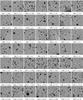 |
Fig. A.1 Finding charts in the Y-band for all 49 objects (crosses) with follow-up spectroscopy. The images are 1 × 1 arcmin2. North is at the top and east is to the left. |
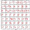 |
Fig. A.2 Light curves of the observed targets with their measurement errors as function of the time since the first available VMC observation. The lines show linear fits to the light curve, following Cioni et al. (2013). |
Observing log for the spectroscopic observations.
All Tables
All Figures
|
Fig. 1 Color–color diagram demonstrating the color selection of quasar candidates. The dashed black lines identify the regions (labeled with letters) where known quasars are found, while the green line marks the blue border of the planetary nebulae locus (Cioni et al. 2013). Our spectroscopically followed up quasars are marked with solid red dots, the non–quasars are marked with red triangles. Blue ×’s indicate the location of the VMC counterparts to the spectroscopically confirmed quasars from Kozłowski et al. (2013), selected adopting a maximum matching radius of 1 arcsec (the average separation is 0.15 ± 0.26 arcsec). Black dots are randomly drawn LMC objects (with errors in all three bands <0.1 mag) to demonstrate the locus of “normal” stars. Contaminating background galaxies are included among the black dots in regions B and C. |
| In the text | |
|
Fig. 2 Location of the spectroscopically followed up quasar candidates in this work (red) and confirmed quasars from Kozłowski et al. (2013) (blue). The VMC tiles are shown as contiguous rectangles. The dashed grid shows lines of constant right ascension (spaced by 15°) and constant declination (spaced by 5°). Coordinates are given with respect to (α0, δ0) = (51°, −69°). |
| In the text | |
|
Fig. 3 Spectra of the quasar candidates sorted by redshift and shifted to rest-frame wavelength. The spectra were normalized to an average value of one and shifted vertically by offsets of two, four, etc., for display purposes. The SDSS composite quasar spectrum (Vanden Berk et al. 2001) is shown at the top of all panels. A sky spectrum is shown at the bottom of the fifth panel (see the next page). Objects with no measured redshift due to lack of lines or low signal-to-noise are plotted assuming z = 0 in the fifth panel next to the sky spectrum to facilitate the identification of the residuals from the sky emission lines. |
| In the text | |
|
Fig. 3 continued. |
| In the text | |
|
Fig. 4 Top: differences between redshifts zi and zj derived from each available pair of lines i and j for objects with multiple lines for bona fide quasars (solid dots) and galaxies (circles). Bottom: redshift histogram for 47 objects in our sample with reliably detected emission lines for bona fide quasars (solid line) and galaxies (dashed line). |
| In the text | |
|
Fig. 5 Histograms of the slope variations (top; the vertical dashed line shows the slope variation limit of 0.0001 mag day-1, adopted in our quasar selection) and the slope uncertainties (bottom) for linear fits to the light curves of the objects in our sample. |
| In the text | |
|
Fig. A.1 Finding charts in the Y-band for all 49 objects (crosses) with follow-up spectroscopy. The images are 1 × 1 arcmin2. North is at the top and east is to the left. |
| In the text | |
|
Fig. A.2 Light curves of the observed targets with their measurement errors as function of the time since the first available VMC observation. The lines show linear fits to the light curve, following Cioni et al. (2013). |
| In the text | |
Current usage metrics show cumulative count of Article Views (full-text article views including HTML views, PDF and ePub downloads, according to the available data) and Abstracts Views on Vision4Press platform.
Data correspond to usage on the plateform after 2015. The current usage metrics is available 48-96 hours after online publication and is updated daily on week days.
Initial download of the metrics may take a while.