| Issue |
A&A
Volume 588, April 2016
|
|
|---|---|---|
| Article Number | A37 | |
| Number of page(s) | 13 | |
| Section | Stellar atmospheres | |
| DOI | https://doi.org/10.1051/0004-6361/201526895 | |
| Published online | 15 March 2016 | |
Abundances of carbon-enhanced metal-poor stars as constraints on their formation⋆
1 Dark Cosmology Centre, The Niels Bohr Institute, Juliane Maries Vej 30, 2100 Copenhagen, Denmark
e-mail: cjhansen@dark-cosmology.dk, birgitta@nbi.ku.dk; ja@nbi.ku.dk
2 Zentrum für Astronomie der Universität Heidelberg, Landessternwarte, Königstuhl 12, 69117 Heidelberg, Germany
3 Stellar Astrophysics Centre, Department of Physics and Astronomy, Aarhus University, Ny Munkegade 120, 8000 Aarhus C, Denmark
4 Research School of Astronomy and Astrophysics, Australian National University, Cotter Road, Weston, ACT 2611, Australia
5 Department of Physics and JINA Center for the Evolution of the Elements, University of Notre Dame, Notre Dame, IN 46556, USA
6 Department of Chemistry, Biochemistry, and Physics, University of Tampa, 401 W. Kennedy Blvd., Tampa, FL 33606, USA
7 Nordic Optical Telescope Scientific Association, Apartado 474, 38700 Santa Cruz de La Palma, Canarias, Spain
8 Leibniz-Institut für Astrophysik Potsdam (AIP), 14482 Potsdam, Germany
9 Centre for Astrophysics Research, Univeristy of Hertfordshire, Hatfield, Herts, AL10 9AB, UK
Received: 3 July 2015
Accepted: 22 November 2015
Context. An increasing fraction of carbon-enhanced metal-poor (CEMP) stars is found as their iron abundance, [Fe/H], decreases below [Fe/H] =−2.0. The CEMP-s stars have the highest absolute carbon abundances, [C/H], and are thought to owe their enrichment in carbon and the slow neutron-capture (s-process) elements to mass transfer from a former asymptotic giant branch (AGB) binary companion. The most Fe-poor CEMP stars are normally single, exhibit somewhat lower [C/H] than CEMP-s stars, but show no s-process element enhancement (CEMP-no stars). Abundance determinations of CNO offer clues to their formation sites.
Aims. Our aim is to use the medium-resolution spectrograph X-Shooter/VLT to determine stellar parameters and abundances for C, N, Sr, and Ba in several classes of CEMP stars in order to further classify and constrain the astrophysical formation sites of these stars.
Methods. Atmospheric parameters for our programme stars were estimated from a combination of V−K photometry, model isochrone fits, and estimates from a modified version of the SDSS/SEGUE spectroscopic pipeline. We then used X-Shooter spectra in conjunction with the 1D local thermodynamic equilibrium spectrum synthesis code MOOG, 1D ATLAS9 atmosphere models to derive stellar abundances, and, where possible, isotopic 12C/13C ratios.
Results. Abundances (or limits) of C, N, Sr, and Ba are derived for a sample of 27 faint metal-poor stars for which the X-Shooter spectra have sufficient signal-to-noise ratios (S/N). These moderate resolution, low S/N (~10−40) spectra prove sufficient to perform limited chemical tagging and enable assignment of these stars into the CEMP subclasses (CEMP-s and CEMP-no). According to the derived abundances, 17 of our sample stars are CEMP-s and 3 are CEMP-no, while the remaining 7 are carbon-normal. For four CEMP stars, the subclassification remains uncertain, and two of them may be pulsating AGB stars.
Conclusions. The derived stellar abundances trace the formation processes and sites of our sample stars. The [C/N] abundance ratio is useful for identifying stars with chemical compositions unaffected by internal mixing, and the [Sr/Ba] abundance ratio allows us to distinguish between CEMP-s stars with AGB progenitors and the CEMP-no stars. Suggested formation sites for the latter include faint supernovae with mixing and fallback and/or primordial, rapidly-rotating, massive stars (spinstars). X-Shooter spectra have thus proved to be valuable tools in the continued search for their origin.
Key words: stars: abundances / stars: Population II / stars: carbon / nuclear reactions, nucleosynthesis, abundances / stars: chemically peculiar
© ESO, 2016
1. Introduction
The class of very metal-poor (VMP; [Fe/H] <−2.0) stars with strong molecular absorption features of carbon, in particular the CH G-band, are collectively referred to as carbon-enhanced metal-poor (CEMP) stars. They are defined as stars with [Fe/H] ≤ −2 and [C/Fe] > 0.7, following Beers & Christlieb (2005) and Aoki et al. (2007), respectively. For convenience, we employ the term “carbonicity” for the carbon-to-iron ratio, [C/Fe], to distinguish it from the absolute carbon abundance, [C/H] (Placco et al. 2011).
In the last two decades it has been recognised that roughly 20% of VMP halo stars exhibit carbonicities up to several orders of magnitude larger than solar (Marsteller et al. 2005; Rossi et al. 2005; Lucatello et al. 2006), rising to 30% for stars with [Fe/H] <−3.0, 40% for [Fe/H] < −3.5, and 75% for [Fe/H] < −4.0. The handful of stars known with [Fe/H] <−5.0 all exhibit large carbonicities (Lee et al. 2013; Placco et al. 2014b; Frebel & Norris 2015), including the most iron-poor star presently known, SMSS J031300.36-670839.3, with [Fe/H] < −7.5 (Keller et al. 2014; Bessell et al. 2015). A definitive interpretation of this increasing frequency has not yet been found, but it has been argued (e.g., Carollo et al. 2012) that CEMP stars are more frequently associated with the outer-halo population of the Galaxy than with the inner-halo population, suggesting differences in the nucleosynthetic production sites of carbon in these components. Carollo et al. (2014) presented indications that the CEMP-s stars are preferentially associated with the inner-halo population, while the CEMP-no stars are associated with the outer-halo population. Based on these, and other recent results (see, e.g., Ito et al. 2013; Placco et al. 2014a; Hansen et al. 2016a), it is becoming increasingly clear that the CEMP-no stars may well be bona fide second-generation stars, born from an interstellar medium (ISM) polluted with the nucleosynthetic products of the very first stars.
A few exceptions to this empirical rule have been presented in Bonifacio et al. (2015) and Caffau et al. (2011). In the former study, a star with an upper limit of [Fe/H] <−5.0 was found to have a low absolute C abundance, while the latter study presented a truly metal-poor star (SDSS J102915+172927) with metallicity slightly above [Fe/H] = −5.0, but without large carbonicity ([C/Fe] ≤ 0.9).
In any event, most results indicate that significant amounts of carbon were already produced at the very earliest stages of the chemical evolution of the Milky Way and the Universe itself. The Galactic chemical evolution (GCE) models by Cescutti et al. (2013) can account for a large amount of the star-to-star scatter in [Sr, Ba/Fe] found at the lowest [Fe/H], and can provide good explanations for the chemistry of most CEMP-no stars, based on a spinstar production scenario (see Cescutti & Chiappini 2010). However, these models alone cannot simultaneously explain the large excess of C, N, and s-process elements found in the CEMP-s stars.
High-resolution spectroscopic studies have shown that ~80% of the known CEMP stars are CEMP-s stars (Aoki et al. 2007, based on their sample of 26 stars). The favoured mechanism to account for these stars is local transfer of carbon-rich material from the envelope of an asymptotic giant-branch (AGB) star to the surface of a surviving binary companion (e.g., Herwig 2005; Bisterzo et al. 2012). Correspondingly, detailed models for the chemical composition of a number of CEMP-s stars have been developed (e.g., Placco et al. 2013, 2015; Abate et al. 2015), but no definitive proof yet exists that they are all members of binary systems (although the vast majority are clearly binaries; see, e.g., Lucatello et al. 2005; Starkenburg et al. 2014). If a given CEMP-s star is not a member of a binary system, eliminating the possibility of mass transfer from an evolved companion, the excess C must have been produced by a distant external source and implanted in the natal cloud of the star observed today.
CEMP-no stars are known to be particularly prevalent among the lowest-metallicity stars (Aoki et al. 2007). Of the nine stars known with [Fe/H] ≤ −4.5, seven are CEMP-no stars (Placco et al. 2014b; Bonifacio et al. 2015; Frebel & Norris 2015), suggesting that C was already produced and enriched in the very first stellar generations. Their low binary frequency (Starkenburg et al. 2014; Hansen et al. 2016a), ~17 ± 5%, consistent with that of halo stars with normal carbon content, and their lack of s-process-element abundance signatures makes a local AGB binary companion an unlikely source of their C excess, so another production site must be found.
Coordinates, photometry, integration times, and resulting S/Ns for our programme stars.
One possible progenitor of the CEMP-no stars are massive, rapidly rotating, mega metal-poor ([Fe/H] <−6.0) stars (Meynet et al. 2006; Hirschi 2007; Frischknecht et al. 2012; Maeder et al. 2015), the so-called spinstars. Another suggested production site for the material incorporated into CEMP-no stars are the so-called faint supernovae associated with the first generations of stars, which experience extensive mixing and fallback during their explosions (e.g., Umeda & Nomoto 2003; Tominaga et al. 2007; Nomoto et al. 2013; Tominaga et al. 2014). It is possible that both of these suggested progenitors may have played a role.
It is noteworthy that extremely metal-poor ([Fe/H] ~−3.0) damped Lyman-α (DLA) systems at high redshift (z = 2−3) with enhanced [C/Fe] (and other light elements) have recently been reported by Cooke et al. (2011, 2012), indicating the existence of a C-enhanced ISM at very early times. Kobayashi et al. (2011) associate C and other elemental abundance signatures of CEMP-no stars with production by faint supernovae, and Matsuoka et al. (2011) have also argued for a strong carbon production in the early Universe based on their analysis of the very distant radio galaxy TN 0924-2201 (z = 5.19)1.
Progress on these issues requires as complete an inventory of the most important elemental- and isotopic-abundance ratios for CEMP stars as possible, in particular C, N, Fe, Sr, Ba, and 12C/13C. The highly efficient X-Shooter instrument on the ESO VLT, covering the full wavelength range from 300 nm to 2.3 μm in a single exposure, allows us to measure the NH band, the CH band, Sr, and Ba in the near-UV to the optical and near-IR.
This paper reports our abundance analysis results for a sample of 27 MP or VMP stars, 20 of which are CEMP stars, and is outlined as follows. Section 2 discusses the target selection for our study. Details of our X-Shooter observations are given in Sect. 3, while Sect. 4 describes our derivation of elemental abundances for the programme stars. Section 5 presents our results, while Sect. 6 offers a discussion of how our key results advance our ultimate goal of understanding the origin of CEMP stars. Finally, our conclusions are presented in Sect. 7.
2. Target selection
Our targets were selected from the “Catalogue of carbon stars found in the Hamburg-ESO survey” (Christlieb et al. 2001) and “Bright Metal-poor Stars from the Hamburg-ESO Survey” (Frebel et al. 2006). For this study we selected the brightest VMP stars, all of which are subgiants or giants, along with a number of additional chemically “normal” metal-poor stars. Initial estimates of atmospheric parameters for most of our candidates were available from application of a modified version of the SEGUE Stellar Parameter Pipeline (n-SSPP), described in more detail below. Based on these estimates, we attempted to select objects in a temperature range suitable for the estimation of molecular abundances such as those from molecular C and N bands. The X-Shooter spectrograph remains efficient even at the NH band at 336 nm, so targets with an effective temperature down to ~4000 K could be observed to a signal-to-noise ratio (S/N) sufficient for abundance analysis in faint stars with reasonable integration times.
The list of our programme stars is given in Table 1, together with the integration times used and the S/Ns (per pixel) obtained. The B and V magnitudes listed are from Beers et al. (2007) unless otherwise stated, while K (=Ks) and J magnitudes are from the 2MASS catalogue (Cutri et al. 2003). After our observations were completed, the star HE 0430−1609 was found to be a single-lined spectroscopic binary with a period of the order of 3 years (Hansen et al. 2016b); this should not affect our results as the low S/N we obtained for this star already yields larger uncertainties.
Our aim was to obtain spectra with sufficient S/N around the NH band at 336 nm, guaranteeing a higher S/N in the redder parts of the wavelength range of X-Shooter. However, measuring an actual S/N from the spectra of cool stars in the near-UV is difficult since the region is extremely crowded with molecular lines and a clean continuum often cannot be defined. We therefore measured the S/N in a region near 400 nm, which still contains a substantial number of mostly molecular lines (see Table 1). This S/N can be taken as representative of the spectrum quality near the Sr line that we employed.
3. Observations and data reduction
The X-Shooter spectrograph is described by Vernet et al. (2011). It has three arms: UV (300–550 nm), visual (550−1000 nm), and near-IR (1000−2500 nm). Our observations were obtained in March and/or August 2010. We used slits of 1′′, 0.9 ′′, and 0.9 ′′in the three arms, yielding resolving powers R = 4350, 7450, and 5300 in the UV, visual, and near-IR spectral regions, respectively. The raw echelle spectra were reduced with the X-Shooter pipeline2, which is an automated routine that performs the necessary data reduction steps, including merging of the orders. The 1D output spectra were extracted, shifted to rest wavelength using cross-correlation with an accuracy of ±1 km s-1, and the continua were normalised in IRAF by dividing the spectra with a fitted pseudo-continuum using cubic splines or Legendre polynomials.
4. Stellar parameters and abundances
The determination of stellar parameters and derivation of stellar abundances were performed with the 1D local thermodynamic equilibrium (LTE) spectrum synthesis code MOOG (Sneden 1973, version 2014), using 1D interpolated Kurucz new opacity distribution function (new-ODF), ATLAS9 model atmospheres (Castelli & Kurucz 2003), calculated with the interpolation code described by Allende Prieto et al. (2004).
4.1. Stellar atmospheric parameter estimates
Extracting stellar atmospheric parameters from the spectra of stars that are dominated by dense forests of molecular bands and absorption lines, in particular for cool stars, is a challenging exercise. Most of the Fe lines normally used for determining [Fe/H] or microturbulence are either saturated or, at our resolving power (R ~ 4350−7450), so heavily blended that we are left with just a handful of usable Fe lines. This is too sparse to use the classical excitation and ionisation equilibrium techniques to estimate the atmospheric parameters, especially since the few useful Fe lines are limited to strong, low excitation-potential lines.
An obvious alternative tracer of [Fe/H] is the Ca triplet at ~855 nm. In our case the triplet lines are of dubious value, as the nearby TiO band is strong in most of our targets, interfering with the continuum placement in this region. Moreover, metallicities derived from the calibrations for red-giant-branch stars by Cole et al. (2004) or for RR Lyrae by Wallerstein et al. (2012) are 0.2–1 dex lower than indicated by the few Fe lines we were able to measure. These apparently spuriously low metallicities resulted in poor spectral fits when synthesising the stellar spectra using such metal-poor atmosphere models.
After much experimentation, we concluded that the best option was either to rebin the optical spectra so that they could be analysed with techniques developed for lower resolution (R ~ 2000) spectra, such as those from SDSS, or else rely on the few useful Fe lines, as described below.
We estimated Teff, log g, and [Fe/H] using the n-SSPP, a modified version of the SEGUE Stellar Parameter Pipeline (SSPP; see e.g., Lee et al. 2008, 2013, for a detailed description of the methods employed). The n-SSPP uses low-resolution optical spectra (typically covering the wavelength range 380−550 nm), which we have for our programme stars, and photometric information (V0, (B−V)0, J0, and (J−K)0, corrected for extinction and reddening based on the Schlegel et al. 1998 dust maps), to determine first-pass estimates for each parameter; the [Fe/H] estimates are particularly important. Typical internal errors for the atmospheric parameters adopted by the n-SSPP are 125 K for Teff, 0.25 dex for log g, 0.20 dex for [Fe/H], and 0.25 dex for [C/Fe]. External errors may well be larger, depending on the wavelength coverage and S/N of the input spectra (see Beers et al. 2014, for further details). However, the n-SSPP pipeline fails for some stars in our sample (in particular those with very low S/N or Teff< 4500 K, outside of the optimal range for the n-SSPP). In such cases, we are forced to derive the stellar parameters in other ways.
The temperatures were finally determined using V−K and the IRFM-based calibrations of Alonso et al. (1999). The E(B−V) were downloaded from the IRSA webpage using the stellar IDs; we adopted the mean E(B−V) values from Schlegel et al. (1998). In the absence of usable trigonometric parallaxes for our stars, we applied the log g−Teff scaling relation from Barklem et al. (2005). However, this relation yielded unrealistically low gravities for some of the stars; we therefore used isochrones, which in most cases agreed with the scaling relation to within 0.2 dex.
We have employed BaSTI (e.g., Pietrinferni et al. 2013) and Padova (Girardi et al. 2000) isochrones with the appropriate metallicities and CNO-enhancements to calculate surface gravities, adopting the photometric temperatures and [Fe/H] from the n-SSPP pipeline. Since the BaSTI isochrones resulted in somewhat larger values of log g for nine stars than expected from the n-SSPP pipeline, we adopted Padova isochrones for metallicities in the range Z = 0.01−0.004. A lower Z in the adopted isochrone leads to a lower gravity. The initial [Fe/H] estimates from the n-SSPP pipeline were adopted, and were adjusted only if the strong Fe lines close to Sr and Ba (e.g., 406.3 and 407.1 nm) indicated a much lower or higher metallicity. In these instances we carried out a spectrum synthesis to fit these Fe lines and updated the [Fe/H] values accordingly. Since these Fe lines are strong, this approach may introduce a bias in our [Fe/H], but these lines remain detectable in our low S/N, moderate-resolution spectra.
In summary, the stellar parameters were determined using photometry, Padova isochrones, and an [Fe/H] estimate based on a combination of the n-SSPP output and by fitting synthetic spectra to a few strong Fe lines near the Sr and Ba lines. The microturbulence was estimated by applying the Gaia-ESO scaling relation between temperature, gravity, metallicity, and microturbulence (Bergemann et al., in prep.). This resulted in values typically between 1.5 and 2.0 km s-1 for most stars. The adopted stellar parameters are thus more uncertain than those derived from high-resolution spectra, and these uncertainties will propagate into the derived stellar abundances (see Sect. 4.3). The final atmospheric parameters are listed in Table 2.
Atmospheric parameters for the programme stars.
Line lists
Before synthetic spectra can be generated, line lists for all relevant features must be assembled. The line list for the molecular bands such as NH, CH, C2, and CN are taken from Masseron et al. (2014) and T. Masseron (priv. comm.). The adopted dissociation energies are 3.47 eV (CH), 3.42 eV (NH), 6.24 eV (C2), and 7.7 eV (CN). The line list covering the atomic lines (Sr and Ba) are from Sneden et al. (2014), with the Sr hyperfine structure from Bergemann et al. (2012) and Hansen et al. (2013), and the Ba hyperfine structure (HFS) from Gallagher et al. (2012). Since most of these stars are of higher metallicities or enriched by an s-process, we used the total solar system isotopic-abundance ratios for the heavy elements.
4.2. Derivation of molecular and atomic stellar abundances
With the ATLAS9 model atmospheres, the above line list, and the stellar parameters in Table 2, the synthetic spectra for each star were computed with MOOG and convolved with a Gaussian representing the X-Shooter resolution at the appropriate wavelength.
Synthetic spectra of the CH G-band (430 nm) and C2 Swan band (516 nm) were fit to the observations to derive the [C/Fe] abundance ratios of our stars, using χ2 minimisation to match the synthetic and the observed spectra across a selected sensitive spectral interval. Nitrogen abundances were estimated in the same way, by fitting synthetic spectra to the NH band around 336 nm and CN around 389 nm and 421 nm, respectively. The listed abundances are average values of these measurements. The stars with low C or N rely only on the strongest CH or NH band, respectively. The isotopic carbon ratios were derived by measuring molecular 13CH features in the range 421–423.5 nm.
Originally, we intended to obtain estimates of O from the CO bands in the near-IR, but the quality of the spectra obtained proved insufficient. We hope to obtain improved spectra in the future from which another attempt to extract O abundances will be made.
The neutron-capture elements Sr and Ba are of particular interest for CEMP stars, as they enable us to distinguish between the CEMP-s and CEMP-no subclasses. Both elements are detectable in the X-Shooter spectra thanks to their strong resonance lines (Hansen et al. 2013). Their abundances were derived via line-by-line spectrum synthesis with line lists including all relevant molecular and atomic lines, and taking into account the HFS of both the Sr and Ba lines. The Sr II line at 407.7 nm is the only useful line of Sr as all other lines are either too weak or are obliterated by strong blends or molecular bands. However, this line is very strong and tends to saturate.
For Ba, we used the two lines at 455.4 nm and 585.3 nm, since they generally yield abundances in good agreement with each other. The 455.4 nm line is the strongest, and is usually detected even in the most metal-poor stars. The 585.3 nm line is weaker, and for this reason possibly more reliable when detectable. The 493.4 nm line is too blended and/or weak to yield reliable abundances, and it was only used to support the upper limit values estimated from the 455.4 nm line when the 585.3 nm line was too weak or blended. Line blends were taken into account by scaling the blends to the overall [Fe/H], α-, r-, and s-process levels when deriving Sr and Ba abundances. Figure 1 shows our spectrum synthesis around the Sr and Ba lines for two programme stars.
4.3. Error propagation
 |
Fig. 1 Synthetic spectrum fits to the Sr II 407.7 nm (upper panel) and Ba II 455.4 nm lines (lower panel). The observations of HE 2141−1441 (relatively metal rich, s-element poor) and HE 0448−4806 (relatively metal poor, s-element rich) are shown as black plus signs. |
The uncertainties listed in Table 4 indicate how well the stellar parameters could be determined, and in turn, how well the abundances could be derived. Several of the stars show signs of variability or are known binaries; in most cases the fit was not as good as it was for the constant VMP stars. The listed uncertainties on the temperature estimates take into account the variability (which could change the magnitudes and thereby the colour of the star) and the uncertainties on the de-reddening. These uncertainties are included with those on the gravities, where a good agreement between Padova and BaSTI isochrones is taken into account; also considered is an agreement between these isocrones and the n-SSPP and the scaled gravities (i.e., the standard deviation around the mean log g is also considered). The uncertainties on the metallicity are estimated from a line-by-line synthesis of the clearly detectable Fe lines in the vicinity of Sr and Ba. The uncertainties have been rounded off in the same way as the stellar parameters.
At the resolving power in the blue arm of X-Shooter (R ~ 4350) all the features of interest are blended to some extent. In particular, features within ~±0.1 nm are blended into the two Sr and Ba lines. These blends affect the Sr line (407.7 nm) the most, and we compensated for the blending caused by La and Dy lines by setting their abundances to that derived from Ba and then adjusted this value by up to 0.3 dex to obtain a better fit of the Sr line.
A minimum abundance error of 0.1 dex due to blends, continuum placement, line list uncertainties, and overall spectrum quality is included in the total error budget, rising to 0.2 dex for the bluest regions of the lowest quality spectra. For poor-quality spectra, the largest uncertainties are due to the stellar parameters (T/log g/[Fe/H]/ξ: ± 300 K/ ± 0.3 dex/ ± 0.3 dex/ ± 0.3 km s-1). In the following we describe our detailed analysis of the maximum abundance uncertainties caused by the stellar parameters for a spectrum of low quality (see Tables 2 and 3).
Abundance sensitivity to stellar parameters for HE 0400−2030.
A minimum uncertainty was estimated using the best spectra and the best-constrained estimates of the stellar atmospheric parameters, and is of the order of T/log g/[Fe/H]/ξ: 100 K/ 0.2 dex/0.1 dex/0.15 km s-1, similar to the uncertainty seen in high-resolution studies and corresponding to our best spectra with a S/N> 30. In this study, most of the stars actually have spectra with S/N ~ 10 at 400 nm, which leads to larger errors. From the minimum and maximum uncertainties we calculated a mean representing the general abundance uncertainty for Sr and Ba.
As seen in Table 3, temperature has the largest impact on the derived abundances. However, Sr and Ba are ionised, so gravity also influences the line strength, but less visibly owing to the blends in the line wings. Microturbulence has the least impact on the Sr and 455.4 nm Ba lines, while the 585.3 nm line of Ba is clearly affected by this parameter. The difference in the sensitivities of the stellar parameters, combined with line blends and varying spectral resolution, explains the small difference in Ba abundances derived from the 455.4 nm line in the blue region ([Ba/Fe] = 1.95) and the 585.3 nm Ba line ([Ba/Fe] ~ 1.7) in the visual region. However, all the Sr and Ba lines agree on the presence or absence of any s-process enhancement, so a star remains enhanced whether or not we consider the blue or visual region of the spectrum.
Finally, we adopted a minimum error of 0.2 dex for the C and N abundances, dominated by the uncertainties on the estimates of the atmospheric parameters.
5. Results
The derived abundances are listed in Table 4. The CEMP classification of Beers & Christlieb (2005), but adopting a lower limit of [C/Fe] > 0.7 as the criterion for CEMP stars (Aoki et al. 2007), leads to 17 CEMP-s stars, 3 CEMP-no stars, and 7 carbon-normal metal-poor stars3 in the total sample. Some of the stars are difficult to fit owing to low S/N, binarity, or pulsations; these stars are identified by a superscript “u” in the table to indicate that the results are more uncertain. The poorer fit to these stars is characterised from a larger standard deviation between the observations and the synthetic MOOG spectra in the range 406–409 nm.
Final stellar parameters, C, N, Sr, and Ba abundances, 12C/13C isotopic ratios, and CEMP classes.
5.1. C and N
In addition to the elemental abundances of C and N, we estimated carbon isotope ratios, 12C/13C, for 13 of our programme stars from 13CH lines in the range 421–423.5 nm; 1 CEMP-no and 12 CEMP-s stars (see Table 4).
All of the stars labelled as CEMP-s have [C/Fe] > 0.7 and [Ba/Fe] > 1.0, which rules out their association with the CEMP-no class. However, three stars exhibit weak Sr absorption lines and almost no Ba features. They are so faint that we can only provide upper limits ([Sr, Ba/Fe] <−3) in one case. These three CEMP-no stars are HE 2155−2043, HE 2250−4229, and HE 2319−5228, discussed in detail in Sect. 6.3. We also identify one very nitrogen-enhanced metal-poor (NEMP) star, HE 0400−2030.
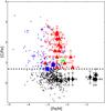 |
Fig. 2 [C/Fe] vs. [Fe/H] for our sample, compared to literature values: Hansen et al. (2015; large open circles) and Placco et al. (2014b and references therein; small open circles). CEMP-s stars are shown in red, CEMP-no stars in blue, the NEMP star in green, and carbon-normal MP stars in black. The dashed line at [C/Fe] = 0.7 separates the VMP and CEMP stars. |
All our programme stars have been checked against the data of Placco et al. (2014b) and Hansen et al. (2015), and the comparison samples used therein (Fig. 2). Figure 3 shows the [C/N] abundance ratio for our programme stars. Two stars, HE 0400−2030 and HE 2319−5228 (discussed in more detail in Sect. 6.3), are found to have mixed CNO-cycled material to their surfaces, converting some C into N (Spite et al. 2005, 2006), while C is normal or enhanced in the rest of the stars. We note that since most of our stars have relatively high gravities (and are subgiants), we do not expect that mixing would alter the surface composition of, e.g., C, and in most cases the C corrections4 from Placco et al. (2014b) are negligible (of the order of 0.0 −0.03 dex). Even for such low-gravity stars as HE 2144−1832, the correction obtained is only ~0.13 dex. Therefore, we have not applied these corrections to any of our abundances.
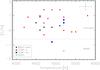 |
Fig. 3 [C/N] ratios determined from our X-Shooter spectra. C-normal MP stars are shown as black diamonds and CEMP-s and CEMP-no as red triangles and blue squares, respectively, while the green cross shows the NEMP star. The dashed line indicates the limit below which CNO-cycled material has been mixed to the surface. |
A summary of our abundance results for C and N is shown in the top two panels of Fig. 4 as functions of [Fe/H].
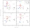 |
Fig. 4 [C, N, Sr, Ba/Fe] ratios vs. [Fe/H] for our programme stars. Chemically normal ([C/Fe] < 0.7) stars are shown in black; red triangles represent CEMP-s stars, and blue squares are CEMP-no stars, and the green “x” symbol is the single NEMP star. The circle marks the uncertain CEMP-no/−s star HE 0516−2515. Dotted lines at [C/Fe] = 0.7 and [Ba/Fe] = 1.0 separate the VMP from the CEMP(-s) stars. |
5.2. Sr and Ba
The Sr and Ba abundances help to distinguish the CEMP-s stars, which have presumably received C-enriched matter transferred from a former AGB companion (Lucatello et al. 2005), from the chemically normal VMP and CEMP-no stars. In contrast, the normal binary frequency of the CEMP-no stars (Starkenburg et al. 2014; Bonifacio et al. 2015; Hansen et al. 2016a) suggests that their abundances reflect the composition of the gas from which they were born.
The derived abundances of Sr and Ba are shown as functions of [Fe/H] in the two lower panels of Fig. 4, in which the metal-poor stars ([C/Fe] < 0.7) are identified by black symbols. At [Fe/H] <−1.5, clear divisions of the Sr and Ba abundances into two branches are seen. Here, the span in Sr and Ba abundances at the lowest [Fe/H] values amounts to ~3 dex (as also found in Hansen et al. 2012), corresponding to the difference between the chemically normal and CEMP-no stars on the one hand, and the highly enhanced CEMP-s stars on the other5. Between the branches is the CEMP-no/s star (for a definition, see Sivarani et al. 2006) HE 0516−2515, with [Ba/Fe] = 0.5 and [Fe/H] = −2.5. Our X-Shooter results for this star are uncertain, and higher-resolution observations are required to classify it with confidence. The blue data points on the low-Sr branch in Fig. 4 are the CEMP-no stars HE 2155−2043 and HE 2250−4229, while HE 2319−5228 falls below this branch. Except for HE 2319−5228, the CEMP-no stars have lower [C/Fe] than the CEMP-s stars.
5.3. Comparison to literature
Our sample has several stars in common with previous studies. Our temperatures generally agree within 150 K with those presented in Goswami (2005), Goswami et al. (2010), and Kennedy et al. (2011). The light-element (C, N) abundances agree within 0.2 dex, while larger differences (up to 0.4 dex) are found among the heavy-element abundances. This large difference can be accounted for by differences in the adopted gravities and metallicities, line lists, and continuum placement. The low resolution of the spectra classified in the study by Goswami et al. (2010) prevented them from deriving accurate metallicities; they estimated these values by comparing the spectra of their high-latitude stars to those with better-known parameters.
Our metallicities also generally agree with those presented in Kennedy et al. (2011) and Aoki et al. (2007) within 0.3 dex. The latter study is based on a high-resolution spectral analysis; we find a fair agreement with most of our results except for the temperatures (owing to differences in adopted E(B−V) values).
All abundances and other parameters derived for HE 1238−0836 are uncertain. The spectra for this star are of low quality and, furthermore, they resemble those of variable RV Tau-type stars6 according to Goswami et al. (2010). The pulsations in such a star can lead to large amplitude changes (and thus magnitude changes) depending on subclass. These variations would in turn lead to very different stellar parameters and abundances, depending on whether the star was observed in an expanding or contracting phase.
Goswami et al. (2010) listed temperatures in the range between 3500 and 4000 K for HE 1238−0836. If the star were as cool as 3500 K when observed with X-Shooter, we would expect to see very strong TiO bands in the red spectra (as in M dwarfs), which we do not. Based on the line profiles (Balmer lines as well as Ba lines) we believe that the star has not been observed at a quiet phase, but we need higher resolution observations during this phase to improve our abundance measurements.
6. Discussion
The recent study of CEMP stars by Spite et al. (2013) showed that, depending on the level of absolute carbon abundance, the stars split into two bands (which they call “plateaus”), where the strongly C-enhanced stars are typically CEMP-s stars, while the relatively less C-enriched stars are CEMP-no stars. Several studies have confirmed the existence of the carbon bands, and have populated them with more stars (e.g., Bonifacio et al. 2015; Hansen et al. 2015). Here we discuss the behaviour of the heavy elements and how they associate with these bands in order to better constrain the astrophysical sites and processes that enriched the different subclasses of CEMP stars. Finally, since our sample also contains carbon-normal VMP stars, we comment on similarities and differences in the formation of VMP stars vs. CEMP stars.
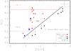 |
Fig. 5 Absolute carbon abundances, A(C) = log ϵ (C), of our programme stars as a function of metallicity, [Fe/H]. The high-C and low-C bands of Spite et al. (2013) are indicated by the horizontal lines. The Asplund et al. (2009) solar abundance of carbon, log ϵ = 8.43, has been assumed. |
Figure 5 shows the absolute C abundances for our programme stars as a function of metallicity, [Fe/H]. The VMP stars are located below the [C/Fe] = 0.7 line. Roughly half of the CEMP-s stars lie close to the high-C band (A(C) = 8.25), while two of our CEMP-no stars are close to the low-C band (A(C) = 6.25). The other CEMP-no stars, the NEMP star, and a few CEMP-s stars fall between the two bands. We do not find any of our programme CEMP-no stars located near the high-C band. Our results and those from other larger studies indicate that there may exist a continuum of absolute C abundances lying between the high- and low-C bands, blurring their distinction.
A discontinuity is seen in both panels of Fig. 6, which illustrates the separation of CEMP-s vs. CEMP-no and VMP stars. The large difference in neutron-capture abundance of 1−2 dex found between C-normal VMP and CEMP-no stars and the CEMP-s stars explains some of the large star-to-star scatter found at low metallicity. This scatter has been found in numerous previous studies, and points towards differences in the formation sites and/or processes involved, if these processes are assumed to be robust and produce similar amounts of heavy elements in each event (see, e.g., Hansen et al. 2014).
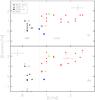 |
Fig. 6 [Sr/Fe] (top) and [Ba/Fe] (bottom) vs. [C/Fe]. The dashed line in the lower panel indicates the limit for s-process enhanced stars at [Ba/Fe] > 1.0. The vertical line at [C/Fe] = 0.7 separates VMP from CEMP stars. |
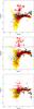 |
Fig. 7 Neutron-capture element abundances vs. [Fe/H] for our stars compared to metal-poor star samples from Hansen et al. (2012, black squares), Hansen et al. (2015, large open circles), and Placco et al. (2014b and references therein, small open circles). Colours and symbols are as in Fig. 2. The red-yellow cloud shows the GCE predictions, where red indicates a larger number density of stars than yellow. The dashed line at [Ba/Fe] = 1.0 in the middle panel separates carbon-normal from CEMP-s stars. The bottom panel shows [Ba/Sr] vs. [Fe/H]. |
Figure 7 compares the X-Shooter measurements of the [Sr/Fe], [Ba/Fe], and [Ba/Sr] abundance ratios for our programme stars to larger samples with high-resolution determinations from Hansen et al. (2012, 2015), and Placco et al. (2014b). As seen from these figures, the CEMP-no stars follow the general trend of stars without C-enhancement predicted by standard Galactic chemical evolution (GCE) models, while the CEMP-s stars increase the star-to-star scatter not just at extremely low metallicities, but over the entire range of [Fe/H]. This is confirmed by the Ba-Sr relation seen in Fig. 9, a relation also found by Roederer (2013) for a much larger sample.
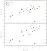 |
Fig. 8 [Sr/H] vs. [C/H] (top) and [Ba/H] vs. [C/H] (bottom). The outlier is HE 2319−5228. |
Both VMP stars and CEMP stars exhibit a steady increase in their neutron-capture elements as a function of time (or [Fe/H]). Figure 8 shows this trend very clearly in terms of the absolute Sr, Ba, and C abundances. Iron has intentionally been excluded from these figures, since Fe is formed in larger amounts by SNe of type Ia, which cannot explain the formation of CEMP-no (or CEMP-s) stars. A possible formation site of the early CEMP-no stars is faint core-collapse SN (type II), which might explode with an O-Ne-Mg core only (e.g., Wanajo et al. 2011), indicating that they will not produce a significant amount of iron. Thus, iron (and its formation processes) might confuse such trends where we look for similarities in abundance ratios to trace the underlying formation process.
Figure 9 shows a difference in the neutron-capture element abundance trends between the C-normal VMP and CEMP-no stars compared to the CEMP-s stars. This would be expected if CEMP-s stars were enriched by a nucleosynthesis process that differs from the process reponsible for enriching metal-poor stars of similar [Fe/H] but lower C-enhancement. The CEMP-s stars are also shown to contain more Ba (a main s-process elements) than Sr (a weak s-process element), yielding a lower [Sr/Ba] ratio and pointing towards early AGB enrichment in a binary system (Lucatello et al. 2005; Masseron et al. 2010; Cristallo et al. 2011; Bisterzo et al. 2012; Starkenburg et al. 2014).
The CEMP-s stars in the top panel of Fig. 9 fall below the Ba-Sr 1:1 relation, while the VMP stars fall above; this is an indication of different formation scenarios that could be hidden in the large star-to-star abundance scatter of Sr and Ba. The CEMP-no stars fall in between these two groups, right on the 1:1 relation.
The ratio of Sr and Ba can be used to trace the formation site – AGB stars vs. spinstars or faint SN II – and the [Ba/Sr] value can even provide insight into the actual mass of the donor AGB star. The predicted [hs/ls] ratio7 from a metal-poor AGB star of 1.5−2M⊙ is ~0.5, according to the Full Network Repository of Updated Isotopic Tables & Yields database (F.R.U.I.T.Y.; Cristallo et al. 2011). Within the observational uncertainty, this is in fair agreement with the observed [Ba/Sr]average ~ 0.45, based on all CEMP-s stars in Fig. 9 (dashed red line). The C-normal VMP stars show the opposite trend ([Ba/Sr]average ~ −0.55; dotted black line). This element ratio could be created by fast-rotating stars, which might produce some Sr and little Ba, depending on conditions such as the rotation velocity (Frischknecht et al. 2012; Piersanti et al. 2013; Cristallo et al. 2015).
These relations are in good agreement with Galactic chemical evolution predictions (Fig. 7), where yields from spinstars may explain the chemically normal stars, but not stars with extreme s-process enhancements (Cescutti et al. 2013; Hansen et al. 2013).
6.1. Comparison to galactic chemical evolution models
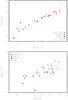 |
Fig. 9 Top: [Sr/H] as a function of [Ba/H]; bottom: [Ba/Sr] as a function of [C/H]. We note the offset in the trends between VMP and the CEMP stars. Two stars in the bottom panel (one VMP and one CEMP-s), lie between the two levels at [C/H] ~2.5; they are the two variable AGB star candidates. The dashed and dotted lines indicate the average [Ba/Sr] ratios of the two groups of stars (see text). |
Figure 7 shows the results from the galactic chemical evolution (GCE) model presented in Cescutti et al. (2013). These results are based on the stochastic enrichment of the ISM, assuming that the pollution by stars are mixed only inside volumes with the radius of a typical SN II bubble (see Cescutti 2008). This model assumes s-process production by spinstars for Sr and Ba, responsible mainly for the region of low [Sr/Fe] and [Ba/Fe] at [Fe/H] <−2.0, coupled with a production of neutron-capture elements by an r-process in electron-capture SNe. By combining yields from these formation sites, the model can account for the dispersion of the data in [Sr/Fe] and [Ba/Fe] for normal stars (and CEMP-no stars)8.
Figure 7 (bottom panel) highlights the importance of the production by spinstars of Sr and Ba at low metallicity coupled with an r-process production. Not only can rotating massive stars at low metallicity produce a modest amount of Sr and Ba (compared to the production of an r-process event), but – even more interestingly – this s-process production also has an [Ba/Sr] ratio varying between 0 and −1.5. As the predictions of the stochastic chemical evolution model show, this is also a solution for the observed dispersion in [Ba/Sr] present in normal stars at extremely low metallicity.
As mentioned above, the chemical evolution model follows the Galactic halo ISM, and therefore cannot predict the enrichment observed in CEMP-s stars. In any case, their atmospheres do not reflect the abundances of the ISM where these stars are formed since the original chemical composition is altered by mass transfer from a binary companion, the most likely formation scenario for the majority of these objects.
6.2. Carbon isotopic ratios, 12C/13C
Convection, either in AGB stars or in spinstars, drives the CNO cycle and transports 13C and N, created at the expense of 12C, to a star’s surface. This is detectable in the isotopic abundance ratios of C and N, where low 12C/13C and [C/N] ratios indicate strong internal mixing with CN-cycled material (Spite et al. 2005). For 13 of our programme CEMP stars we find ratios that cover 3 <12C/13C < 50, where the higher end of this range is in good agreement with Bisterzo et al. (2011, 2012), who find that their AGB models without strong mixing do not result in the low, observed values (4 <12C/13C < 10).
The equilibrium value of 12C/13C for CNO-cycled material is 3−4, so stars with 12C/13C = 5 indicate a high level of processing. This either points towards more processing in the AGB stars than current models predict or it indicates processing by the star itself. Seven stars (HE 0058−3449, HE 0241−3512, HE 0400−2030, HE 0414−0343, HE 0440−3426, HE 0448−4806, HE 2319−5228) exhibit 12C/13C ratios <10; two of these are subgiants and five are giants; some degree of internal processing is expected in all seven of them. In Fig. 3 we note that HE 0400−2030 and HE 2319−5228 showed clear signs of mixing.
Two stars stand out by having a low log g and a positive [C/N] ratio, namely HE 1238−0836 and HE 2144−1832. Both of these stars are also photometric variables. According to Goswami et al. (2010), HE 1238−0836 is an RV Tau-type (R Sct) star; such stars can exhibit extreme variations in their light curves. As mentioned in Sect. 5.3, we expect to have observed the star in (or close to) an expansion phase, where the gravity and in turn the pressure-sensitive abundances are too low. Multi-epoch follow-up observations would be needed to verify the variable character. We need to observe the star in a quiet phase when the derived stellar parameters and abundances can be trusted. However, there is also another possibility. Both stars could be pulsating, intrinsic AGB stars such as CS 30322-023 (Masseron et al. 2006) and HD 112869 (Začs et al. 2015). This would explain their low gravities and their high levels of brightness (both stars are brighter than most other stars in our programme). Either option could lead to [C/N] > 0, and would most likely result in high 12C/13C-ratios.
6.3. CEMP-no and NEMP stars
To date we know ~80 CEMP-no stars (most of which have been included in Placco et al. 2014b)9. Not all of them are confirmed CEMP-no stars, but the majority are expected to belong to this subclass. Our confirmation of three new CEMP-no stars (HE 2155−2043, HE 2250−4229, and HE 2319−5228) adds to this sample. The nature of the progenitors that enriched the ISM from which such stars formed (faint SNe with mixing and fallback, and/or spinstars) is still not fully understood.
In the spinstars scenario, rotation triggers mixing processes inside the star, and this leads to the production of important quantities of primary 14N, 13C, and 22Ne compared to stellar evolution models without rotation (Hirschi 2007). However, this scenario does not fit the abundance pattern of one of the most-studied CEMP-no stars, BD+44°493 (Ito et al. 2013; Placco et al. 2014a; Maeder & Meynet 2015). Ito et al. (2013) found a nitrogen enhancement in this star that is too low with respect to the carbon enhancement to match these predictions. The abundance pattern of HE 2319−5228, however, appears to be consistent with a spinstar progenitor that may have been present in the earliest generations of stars (e.g., Maeder et al. 2015).
The NEMP star: HE 0400−2030
Johnson et al. (2007) defined the NEMP stars as objects with [C/N] ≲−0.5 and [N/Fe] > 0.5, and found five examples. This number was lower than expected, and seemed to point towards an observational bias against discovering NEMP stars relative to CEMP stars (which are more readily identifiable from objective-prism surveys). However, the number of recognised NEMP stars has increased to ~45 at present (Placco et al. 2014b), which is a substantial number, although still less than the number of known CEMP-no and CEMP-s stars. We find one new NEMP star: HE 0400−2030, which has [C/N] = −1.4 and is also s-process-element enhanced.
6.4. Comparison to AGB yields
As a result of hot bottom burning (HBB), the higher mass stars (of 4−6 M⊙) produce prodigious amounts of nitrogen at the expense of carbon. A few CEMP stars studied to date exhibit abundance patterns that could be consistent with these higher mass AGB stars, but the stars in our X-Shooter sample appear to be largely consistent with the 1.5–3 M⊙ cases where nitrogen is not enhanced relative to carbon, as would be expected from a HBB scenario.
Among the seven stars that show indications of mixing through their [C/N] ratios or isotopic carbon-abundance ratios, none exhibit [C/N] < −0.5 and [hs/ls] > 0.5 simultaneously. This indicates that HBB in more massive stars (≳4 M⊙) is a less plausible explanation for the chemical composition of these stars. Most of our programme stars exhibit signs of weak internal mixing, which, based on their [Ba/Sr] ([hs/ls]) ratios, can be explained by either AGB stars, massive spinstars, or faint SNe with mixing and fallback.
7. Conclusions
Twenty-seven stars from our X-Shooter programme were analysed through spectral synthesis of molecular C and N bands, and atomic Ba and Sr lines. With only these four abundances, it is possible to classify each star according to its abundance pattern (i.e., CEMP-s, CEMP-no etc.). The majority of the known CEMP stars are enriched in s-process elements such as Ba and Sr. These CEMP-s stars appear to belong to the relatively metal-rich inner-halo population, while the CEMP-no stars may belong primarily to the relatively more metal-poor outer-halo population (e.g., Carollo et al. 2012, 2014).
Despite intense efforts to date, we are still trying to understand the exact formation sites of the CEMP-no and NEMP stars. Two of our newly confirmed CEMP-no stars appear to fall on (or slightly above) the low-C band suggested by Spite et al. (2013). We also confirm the differences found between the strongly C-enhanced CEMP-s stars and the relatively less C-enhanced CEMP-no stars discussed by the same authors. However, several stars in this and other larger studies appear to indicate a continuum of absolute C abundances rather than discrete bands. Here we show that differences in the heavy element abundances as a function of the absolute carbon abundances ([C/H]) show similar plateau trends for the two subclasses of CEMP stars. We note that larger samples may erase these plateaus and exhibit more continouos distributions around similar average values.
Comparison of the CEMP-s stars to AGB model yields (e.g., Cristallo et al. 2011) indicates that the progenitor AGB stars were primarily of the lower mass variety (in agreement with Kennedy et al. 2011 and Bisterzo et al. 2012), while the NEMP star in our programme could be associated with a more massive AGB progenitor capable of producing large abundances of nitrogen relative to carbon. However, the [hs/ls] ratio for this star agrees with values predicted for lower mass AGB stars (~2 M⊙). The two stars with low gravities (HE 1238−0836 and HE 2144−1832) appear to be pulsating variables, which could yield more trustworthy abundances if observed in a quiet phase. They could also be intrinsic AGB stars.
This study has shown that moderate-resolution, low S/N X-Shooter spectra are of sufficient quality to classify CEMP stars into subcatogories and to extract information on their plausible astrophysical formation sites, which highlights an aspect of the X-Shooter instrument that we consider very promising: the ability to obtain simultaneous measurements of C, N, Ba, and Sr very efficiently for a relatively large sample of faint stars. This is important, in particular for intermediate- to low-metallicity −2.5 < [Fe/H] < −1.0 stars, a range we cover with our sample. This metallicity interval has been largely ignored in recent observational campaigns that concentrate on the most extreme metal-poor stars. Substantial and crucial information can be extracted at intermediate metallicity, where numerous stars of the halo system are found. For example, different r-process sites predict dispersions in stellar abundances of [Sr/H] or [Ba/H], as discussed by Cescutti & Chiappini (2014) and Hansen et al. (2012, 2014).
Carbon ([CII]) is also measured at even higher redshifts (z ~ 7.1) in a quasar (J112001.48+064124.3), and is found to be lower than in other quasars at z ~ 6 (Venemans et al. 2012). The carbon-to-far-infrared flux ratio indicates the presence of a significant amount of cold gas and dust in the early Universe.
These results are independent of other proposed r-process sites (see, e.g., Cescutti & Chiappini 2014) combined with spinstars. This was confirmed in Cescutti et al. (2015) using neutron star mergers as an r-process site. Similar results can be obtained considering only two different primary (r-)process contributions not involving spinstars (see, e.g., Hansen & Primas 2011; Hansen et al. 2014).
Many studies over the past decades have steadily added to this sample, e.g., Norris et al. (1997, 2007), Christlieb et al. (2002), Frebel et al. (2005), Aoki et al. (2007), Ito et al. (2013), Yong et al. (2013), Keller et al. (2014), Placco et al. (2014b), Bonifacio et al. (2015), Hansen et al. (2015), Li et al. (2015).
Acknowledgments
C.J.H. acknowledges support from research grant VKR023371 from the Villum Foundation, and both she and T.T.H. acknowledge support from Sonderforschungsbereich SFB 881. “The Milky Way System” (subproject A5) of the German Research Foundation (DFG). B.N. and C.J.H. thank Drs. J. Fynbo and D. Malesani for help with the X-Shooter observations. B.N. acknowledges partial support by the National Science Foundation under Grant No. NSF PHY11-25915. T.T.H. thanks T. Masseron for line list information. T.C.B., C.R.K., and V.M.P. acknowledge partial funding of this work from grants PHY 08-22648; Physics Frontier Center/Joint Institute or Nuclear Astrophysics (JINA), and PHY 14-30152; Physics Frontier Center/JINA Center for the Evolution of the Elements (JINA-CEE), awarded by the US National Science Foundation. J.A. and B.N. acknowledge support from the Danish Council for Independent Research | Natural Sciences and the Carlsberg Foundation. This publication has made use of the SIMBAD database, operated at CDS, Strasbourg, France, and of data products from the Two Micron All Sky Survey, which is a joint project of the University of Massachusetts and the Infrared Processing and Analysis Center/California Institute of Technology, funded by the National Aeronautics and Space Administration and the National Science Foundation.
References
- Abate, C., Pols, O. R., Karakas, A. I., & Izzard, R. G. 2015, A&A, 576, A118 [NASA ADS] [CrossRef] [EDP Sciences] [Google Scholar]
- Allen de Prieto, C., Barklem, P. S., Lambert, D. L., & Cunha, K. 2004, A&A, 420, 183 [NASA ADS] [CrossRef] [EDP Sciences] [Google Scholar]
- Alonso, A., Arribas, S., & Martínez-Roger, C. 1999, A&AS, 140, 261 [NASA ADS] [CrossRef] [EDP Sciences] [Google Scholar]
- Aoki, W., Beers, T. C., Christlieb, N., et al. 2007, ApJ, 655, 492 [NASA ADS] [CrossRef] [Google Scholar]
- Asplund, M., Grevesse, N., Sauval, A. J., & Scott, P. 2009, ARA&A, 47, 481 [NASA ADS] [CrossRef] [Google Scholar]
- Barklem, P. S., Christlieb, N., Beers, T. C., et al. 2005, A&A, 439, 129 [NASA ADS] [CrossRef] [EDP Sciences] [Google Scholar]
- Beers, T. C., & Christlieb, N. 2005, ARA&A, 43, 531 [NASA ADS] [CrossRef] [Google Scholar]
- Beers, T. C., Flynn, C., Rossi, S., et al. 2007, ApJS, 168, 128 [NASA ADS] [CrossRef] [Google Scholar]
- Beers, T. C., Norris, J. E., Placco, V. M., et al. 2014, ApJ, 794, 58 [NASA ADS] [CrossRef] [Google Scholar]
- Bergemann, M., Hansen, C. J., Bautista, M., & Ruchti, G. 2012, A&A, 546, A90 [NASA ADS] [CrossRef] [EDP Sciences] [Google Scholar]
- Bessell, M. S., Collet, R., Keller, S. C., et al. 2015, ApJ, 806, L16 [NASA ADS] [CrossRef] [Google Scholar]
- Bisterzo, S., Gallino, R., Straniero, O., Cristallo, S., & Käppeler, F. 2011, MNRAS, 418, 284 [NASA ADS] [CrossRef] [Google Scholar]
- Bisterzo, S., Gallino, R., Straniero, O., Cristallo, S., & Käppeler, F. 2012, MNRAS, 422, 849 [NASA ADS] [CrossRef] [Google Scholar]
- Bonifacio, P., Caffau, E., Spite, M., et al. 2015, A&A, 579, A28 [NASA ADS] [CrossRef] [EDP Sciences] [Google Scholar]
- Caffau, E., Bonifacio, P., François, P., et al. 2011, Nature, 477, 67 [NASA ADS] [CrossRef] [PubMed] [Google Scholar]
- Carollo, D., Beers, T. C., Bovy, J., et al. 2012, ApJ, 744, 195 [NASA ADS] [CrossRef] [Google Scholar]
- Carollo, D., Freeman, K., Beers, T. C., et al. 2014, ApJ, 788, 180 [NASA ADS] [CrossRef] [Google Scholar]
- Castelli, F., & Kurucz, R. L. 2003, in Modelling of Stellar Atmospheres, eds. N. Piskunov, W. W. Weiss, & D. F. Gray, IAU Symp., 210, 20 [Google Scholar]
- Cescutti, G. 2008, A&A, 481, 691 [NASA ADS] [CrossRef] [EDP Sciences] [Google Scholar]
- Cescutti, G., & Chiappini, C. 2010, A&A, 515, A102 [NASA ADS] [CrossRef] [EDP Sciences] [Google Scholar]
- Cescutti, G., & Chiappini, C. 2014, A&A, 565, A51 [NASA ADS] [CrossRef] [EDP Sciences] [Google Scholar]
- Cescutti, G., Chiappini, C., Hirschi, R., Meynet, G., & Frischknecht, U. 2013, A&A, 553, A51 [NASA ADS] [CrossRef] [EDP Sciences] [Google Scholar]
- Cescutti, G., Romano, D., Matteucci, F., Chiappini, C., & Hirschi, R. 2015, A&A, 577, A139 [NASA ADS] [CrossRef] [EDP Sciences] [Google Scholar]
- Christlieb, N., Green, P. J., Wisotzki, L., & Reimers, D. 2001, A&A, 375, 366 [NASA ADS] [CrossRef] [EDP Sciences] [Google Scholar]
- Christlieb, N., Bessell, M. S., Beers, T. C., et al. 2002, Nature, 419, 904 [NASA ADS] [CrossRef] [PubMed] [Google Scholar]
- Cole, A. A., Smecker-Hane, T. A., Tolstoy, E., Bosler, T. L., & Gallagher, J. S. 2004, MNRAS, 347, 367 [NASA ADS] [CrossRef] [Google Scholar]
- Cooke, R., Pettini, M., Steidel, C. C., Rudie, G. C., & Nissen, P. E. 2011, MNRAS, 417, 1534 [NASA ADS] [CrossRef] [Google Scholar]
- Cooke, R., Pettini, M., & Murphy, M. T. 2012, MNRAS, 425, 347 [NASA ADS] [CrossRef] [Google Scholar]
- Cristallo, S., Piersanti, L., Straniero, O., et al. 2011, ApJS, 197, 17 [NASA ADS] [CrossRef] [Google Scholar]
- Cristallo, S., Abia, C., Straniero, O., & Piersanti, L. 2015, ApJ, 801, 53 [NASA ADS] [CrossRef] [Google Scholar]
- Cutri, R. M., Skrutskie, M. F., van Dyk, S., et al. 2003, VizieR Online Data Catalog: II/246 [Google Scholar]
- Frebel, A., & Norris, J. E. 2015, ARA&A, 53, 631 [NASA ADS] [CrossRef] [Google Scholar]
- Frebel, A., Aoki, W., Christlieb, N., et al. 2005, Nature, 434, 871 [NASA ADS] [CrossRef] [PubMed] [Google Scholar]
- Frebel, A., Christlieb, N., Norris, J. E., et al. 2006, ApJ, 652, 1585 [NASA ADS] [CrossRef] [Google Scholar]
- Frischknecht, U., Hirschi, R., & Thielemann, F.-K. 2012, A&A, 538, L2 [NASA ADS] [CrossRef] [EDP Sciences] [Google Scholar]
- Gallagher, A. J., Ryan, S. G., Hosford, A., et al. 2012, A&A, 538, A118 [NASA ADS] [CrossRef] [EDP Sciences] [Google Scholar]
- Girardi, L., Bressan, A., Bertelli, G., & Chiosi, C. 2000, A&AS, 141, 371 [NASA ADS] [CrossRef] [EDP Sciences] [Google Scholar]
- Goswami, A. 2005, MNRAS, 359, 531 [NASA ADS] [CrossRef] [Google Scholar]
- Goswami, A., Karinkuzhi, D., & Shantikumar, N. S. 2010, MNRAS, 402, 1111 [NASA ADS] [CrossRef] [Google Scholar]
- Hansen, C. J., & Primas, F. 2011, A&A, 525, L5 [NASA ADS] [CrossRef] [EDP Sciences] [Google Scholar]
- Hansen, C. J., Primas, F., Hartman, H., et al. 2012, A&A, 545, A31 [NASA ADS] [CrossRef] [EDP Sciences] [Google Scholar]
- Hansen, C. J., Bergemann, M., Cescutti, G., et al. 2013, A&A, 551, A57 [NASA ADS] [CrossRef] [EDP Sciences] [Google Scholar]
- Hansen, C. J., Montes, F., & Arcones, A. 2014, ApJ, 797, 123 [NASA ADS] [CrossRef] [Google Scholar]
- Hansen, T., Hansen, C. J., Christlieb, N., et al. 2015, ApJ, 807, 173 [NASA ADS] [CrossRef] [Google Scholar]
- Hansen, T. T., Andersen, J., Nordström, B., et al. 2016a, A&A, 586, A160 [NASA ADS] [CrossRef] [EDP Sciences] [Google Scholar]
- Hansen, T., Andersen, J., Nordström, B., et al. 2016b, A&A, 588, A3 [NASA ADS] [CrossRef] [EDP Sciences] [Google Scholar]
- Henden, A. A., Levine, S., Terrell, D., & Welch, D. L. 2015, in AAS Meeting, 225, 336.16 [Google Scholar]
- Herwig, F. 2005, ARA&A, 43, 435 [NASA ADS] [CrossRef] [Google Scholar]
- Hirschi, R. 2007, A&A, 461, 571 [NASA ADS] [CrossRef] [EDP Sciences] [Google Scholar]
- Hollek, J. K., Frebel, A., Placco, V. M., et al. 2015, ApJ, 814, 121 [NASA ADS] [CrossRef] [Google Scholar]
- Ito, H., Aoki, W., Beers, T. C., et al. 2013, ApJ, 773, 33 [NASA ADS] [CrossRef] [Google Scholar]
- Johnson, J. A., Herwig, F., Beers, T. C., & Christlieb, N. 2007, ApJ, 658, 1203 [NASA ADS] [CrossRef] [Google Scholar]
- Keller, S. C., Bessell, M. S., Frebel, A., et al. 2014, Nature, 506, 463 [NASA ADS] [CrossRef] [PubMed] [Google Scholar]
- Kennedy, C. R., Sivarani, T., Beers, T. C., et al. 2011, AJ, 141, 102 [NASA ADS] [CrossRef] [Google Scholar]
- Kobayashi, C., Tominaga, N., & Nomoto, K. 2011, ApJ, 730, L14 [NASA ADS] [CrossRef] [Google Scholar]
- Lee, Y. S., Beers, T. C., Sivarani, T., et al. 2008, AJ, 136, 2022 [NASA ADS] [CrossRef] [Google Scholar]
- Lee, Y. S., Beers, T. C., Masseron, T., et al. 2013, AJ, 146, 132 [NASA ADS] [CrossRef] [Google Scholar]
- Li, H., Aoki, W., Zhao, G., et al. 2015, PASJ, 67, 84 [NASA ADS] [CrossRef] [Google Scholar]
- Lucatello, S., Tsangarides, S., Beers, T. C., et al. 2005, ApJ, 625, 825 [NASA ADS] [CrossRef] [Google Scholar]
- Lucatello, S., Beers, T. C., Christlieb, N., et al. 2006, ApJ, 652, L37 [NASA ADS] [CrossRef] [Google Scholar]
- Maeder, A., & Meynet, G. 2015, A&A, 580, A32 [NASA ADS] [CrossRef] [EDP Sciences] [Google Scholar]
- Maeder, A., Meynet, G., & Chiappini, C. 2015, A&A, 576, A56 [NASA ADS] [CrossRef] [EDP Sciences] [Google Scholar]
- Marsteller, B., Beers, T. C., Rossi, S., et al. 2005, Nucl. Phys. A, 758, 312 [NASA ADS] [CrossRef] [Google Scholar]
- Masseron, T., van Eck, S., Famaey, B., et al. 2006, A&A, 455, 1059 [NASA ADS] [CrossRef] [EDP Sciences] [Google Scholar]
- Masseron, T., Johnson, J. A., Plez, B., et al. 2010, A&A, 509, A93 [NASA ADS] [CrossRef] [EDP Sciences] [Google Scholar]
- Masseron, T., Plez, B., Van Eck, S., et al. 2014, A&A, 571, A47 [NASA ADS] [CrossRef] [EDP Sciences] [Google Scholar]
- Matsuoka, K., Nagao, T., Maiolino, R., Marconi, A., & Taniguchi, Y. 2011, A&A, 532, L10 [NASA ADS] [CrossRef] [EDP Sciences] [Google Scholar]
- Meynet, G., Ekström, S., & Maeder, A. 2006, A&A, 447, 623 [NASA ADS] [CrossRef] [EDP Sciences] [Google Scholar]
- Nomoto, K., Kobayashi, C., & Tominaga, N. 2013, ARA&A, 51, 457 [NASA ADS] [CrossRef] [Google Scholar]
- Norris, J. E., Ryan, S. G., & Beers, T. C. 1997, ApJ, 489, L169 [NASA ADS] [CrossRef] [Google Scholar]
- Norris, J. E., Christlieb, N., Korn, A. J., et al. 2007, ApJ, 670, 774 [NASA ADS] [CrossRef] [Google Scholar]
- Piersanti, L., Cristallo, S., & Straniero, O. 2013, ApJ, 774, 98 [NASA ADS] [CrossRef] [Google Scholar]
- Pietrinferni, A., Cassisi, S., Salaris, M., & Hidalgo, S. 2013, A&A, 558, A46 [NASA ADS] [CrossRef] [EDP Sciences] [Google Scholar]
- Placco, V. M., Kennedy, C. R., Beers, T. C., et al. 2011, AJ, 142, 188 [NASA ADS] [CrossRef] [Google Scholar]
- Placco, V. M., Frebel, A., Beers, T. C., et al. 2013, ApJ, 770, 104 [NASA ADS] [CrossRef] [Google Scholar]
- Placco, V. M., Beers, T. C., Roederer, I. U., et al. 2014a, ApJ, 790, 34 [NASA ADS] [CrossRef] [Google Scholar]
- Placco, V. M., Frebel, A., Beers, T. C., & Stancliffe, R. J. 2014b, ApJ, 797, 21 [NASA ADS] [CrossRef] [Google Scholar]
- Placco, V. M., Beers, T. C., Ivans, I. I., et al. 2015, ApJ, 812, 109 [NASA ADS] [CrossRef] [Google Scholar]
- Roederer, I. U. 2013, AJ, 145, 26 [NASA ADS] [CrossRef] [Google Scholar]
- Rossi, S., Beers, T. C., Sneden, C., et al. 2005, AJ, 130, 2804 [NASA ADS] [CrossRef] [Google Scholar]
- Schlegel, D. J., Finkbeiner, D. P., & Davis, M. 1998, ApJ, 500, 525 [NASA ADS] [CrossRef] [Google Scholar]
- Sivarani, T., Beers, T. C., Bonifacio, P., et al. 2006, A&A, 459, 125 [NASA ADS] [CrossRef] [EDP Sciences] [Google Scholar]
- Sneden, C. A. 1973, Ph.D. Thesis, The University of Texas at Austin [Google Scholar]
- Sneden, C., Lucatello, S., Ram, R. S., Brooke, J. S. A., & Bernath, P. 2014, ApJS, 214, 26 [Google Scholar]
- Spite, M., Cayrel, R., Plez, B., et al. 2005, A&A, 430, 655 [NASA ADS] [CrossRef] [EDP Sciences] [Google Scholar]
- Spite, M., Cayrel, R., Hill, V., et al. 2006, A&A, 455, 291 [NASA ADS] [CrossRef] [EDP Sciences] [Google Scholar]
- Spite, M., Caffau, E., Bonifacio, P., et al. 2013, A&A, 552, A107 [NASA ADS] [CrossRef] [EDP Sciences] [Google Scholar]
- Starkenburg, E., Shetrone, M. D., McConnachie, A. W., & Venn, K. A. 2014, MNRAS, 441, 1217 [NASA ADS] [CrossRef] [Google Scholar]
- Tominaga, N., Umeda, H., & Nomoto, K. 2007, ApJ, 660, 516 [NASA ADS] [CrossRef] [Google Scholar]
- Tominaga, N., Iwamoto, N., & Nomoto, K. 2014, ApJ, 785, 98 [NASA ADS] [CrossRef] [Google Scholar]
- Umeda, H., & Nomoto, K. 2003, Nature, 422, 871 [NASA ADS] [CrossRef] [PubMed] [Google Scholar]
- Venemans, B. P., McMahon, R. G., Walter, F., et al. 2012, ApJ, 751, L25 [Google Scholar]
- Vernet, J., Dekker, H., D’Odorico, S., et al. 2011, A&A, 536, A105 [NASA ADS] [CrossRef] [EDP Sciences] [Google Scholar]
- Wallerstein, G., Gomez, T., & Huang, W. 2012, Ap&SS, 341, 89 [NASA ADS] [CrossRef] [Google Scholar]
- Wanajo, S., Janka, H.-T., & Müller, B. 2011, ApJ, 726, L15 [NASA ADS] [CrossRef] [Google Scholar]
- Yong, D., Norris, J. E., Bessell, M. S., et al. 2013, ApJ, 762, 26 [NASA ADS] [CrossRef] [Google Scholar]
- Začs, L., Sperauskas, J., Grankina, A., et al. 2015, ApJ, 803, 17 [NASA ADS] [CrossRef] [Google Scholar]
All Tables
Coordinates, photometry, integration times, and resulting S/Ns for our programme stars.
Final stellar parameters, C, N, Sr, and Ba abundances, 12C/13C isotopic ratios, and CEMP classes.
All Figures
|
Fig. 1 Synthetic spectrum fits to the Sr II 407.7 nm (upper panel) and Ba II 455.4 nm lines (lower panel). The observations of HE 2141−1441 (relatively metal rich, s-element poor) and HE 0448−4806 (relatively metal poor, s-element rich) are shown as black plus signs. |
| In the text | |
|
Fig. 2 [C/Fe] vs. [Fe/H] for our sample, compared to literature values: Hansen et al. (2015; large open circles) and Placco et al. (2014b and references therein; small open circles). CEMP-s stars are shown in red, CEMP-no stars in blue, the NEMP star in green, and carbon-normal MP stars in black. The dashed line at [C/Fe] = 0.7 separates the VMP and CEMP stars. |
| In the text | |
|
Fig. 3 [C/N] ratios determined from our X-Shooter spectra. C-normal MP stars are shown as black diamonds and CEMP-s and CEMP-no as red triangles and blue squares, respectively, while the green cross shows the NEMP star. The dashed line indicates the limit below which CNO-cycled material has been mixed to the surface. |
| In the text | |
|
Fig. 4 [C, N, Sr, Ba/Fe] ratios vs. [Fe/H] for our programme stars. Chemically normal ([C/Fe] < 0.7) stars are shown in black; red triangles represent CEMP-s stars, and blue squares are CEMP-no stars, and the green “x” symbol is the single NEMP star. The circle marks the uncertain CEMP-no/−s star HE 0516−2515. Dotted lines at [C/Fe] = 0.7 and [Ba/Fe] = 1.0 separate the VMP from the CEMP(-s) stars. |
| In the text | |
|
Fig. 5 Absolute carbon abundances, A(C) = log ϵ (C), of our programme stars as a function of metallicity, [Fe/H]. The high-C and low-C bands of Spite et al. (2013) are indicated by the horizontal lines. The Asplund et al. (2009) solar abundance of carbon, log ϵ = 8.43, has been assumed. |
| In the text | |
|
Fig. 6 [Sr/Fe] (top) and [Ba/Fe] (bottom) vs. [C/Fe]. The dashed line in the lower panel indicates the limit for s-process enhanced stars at [Ba/Fe] > 1.0. The vertical line at [C/Fe] = 0.7 separates VMP from CEMP stars. |
| In the text | |
|
Fig. 7 Neutron-capture element abundances vs. [Fe/H] for our stars compared to metal-poor star samples from Hansen et al. (2012, black squares), Hansen et al. (2015, large open circles), and Placco et al. (2014b and references therein, small open circles). Colours and symbols are as in Fig. 2. The red-yellow cloud shows the GCE predictions, where red indicates a larger number density of stars than yellow. The dashed line at [Ba/Fe] = 1.0 in the middle panel separates carbon-normal from CEMP-s stars. The bottom panel shows [Ba/Sr] vs. [Fe/H]. |
| In the text | |
|
Fig. 8 [Sr/H] vs. [C/H] (top) and [Ba/H] vs. [C/H] (bottom). The outlier is HE 2319−5228. |
| In the text | |
|
Fig. 9 Top: [Sr/H] as a function of [Ba/H]; bottom: [Ba/Sr] as a function of [C/H]. We note the offset in the trends between VMP and the CEMP stars. Two stars in the bottom panel (one VMP and one CEMP-s), lie between the two levels at [C/H] ~2.5; they are the two variable AGB star candidates. The dashed and dotted lines indicate the average [Ba/Sr] ratios of the two groups of stars (see text). |
| In the text | |
Current usage metrics show cumulative count of Article Views (full-text article views including HTML views, PDF and ePub downloads, according to the available data) and Abstracts Views on Vision4Press platform.
Data correspond to usage on the plateform after 2015. The current usage metrics is available 48-96 hours after online publication and is updated daily on week days.
Initial download of the metrics may take a while.