| Issue |
A&A
Volume 587, March 2016
|
|
|---|---|---|
| Article Number | A89 | |
| Number of page(s) | 15 | |
| Section | Planets and planetary systems | |
| DOI | https://doi.org/10.1051/0004-6361/201527388 | |
| Published online | 23 February 2016 | |
Orbital fitting of imaged planetary companions with high eccentricities and unbound orbits
Their application to Fomalhaut b and PZ Telecopii B⋆
1 Univ. Grenoble Alpes, IPAG, 38000 Grenoble, France
e-mail: This email address is being protected from spambots. You need JavaScript enabled to view it.
2 CNRS, IPAG, 38000 Grenoble, France
3 INAF–Osservatorio Astronomico de Padova, Vicolo dell’Osservatorio 5, 35122 Padova, Italy
4 Observatoire de Genève, Université de Genève, 51 Ch. des Maillettes, 1290 Sauverny, Switzerland
Received: 17 September 2015
Accepted: 10 December 2015
Abstract
Context. Regular follow-up of imaged companions to main-sequence stars often allows a projected orbital motion to be detected. Markov chain Monte Carlo (MCMC) has become very popular recent years for fitting and constraining their orbits. Some of these imaged companions appear to move on very eccentric, possibly unbound orbits. This is, in particular, the case for the exoplanet Fomalhaut b and the brown dwarf companion PZ Tel B on which we focus here.
Aims. For these orbits, standard MCMC codes that assume only bound orbits may be inappropriate. Our goal is to develop a new MCMC implementation that is able to handle both bound and unbound orbits in a continuous manner, and to apply this to the cases of Fomalhaut b and PZ Tel B.
Methods. We present here this code, based on the use of universal Keplerian variables and Stumpff functions. We present two versions of this code, the second one using a different set of angular variables that were designed to avoid degeneracies arising when the projected orbital motion is quasi-radial, as is the case for PZ Tel B. We also present additional observations of PZ Tel B.
Results. The code is applied to Fomalhaut b and PZ Tel B. We confirm previous results in relation to, but we show that on the sole basis of the astrometric data, open orbital solutions are also possible. The eccentricity distribution nevertheless still peaks around ~0.9 in the bound regime. We present a first successful orbital fit of PZ Tel B, which shows in particular that, while both bound and unbound orbital solutions are equally possible, the eccentricity distribution presents a sharp peak very close to e = 1, meaning a quasi-parabolic orbit.
Conclusions. It has recently been suggested that the presence of unseen inner companions to imaged ones may lead orbital fitting algorithms to artificially give very high eccentricities. We show that this caveat is unlikely to apply to Fomalhaut b. Concerning PZ Tel B, we derive a possible solution, which involves an inner ~12 MJup companion, that would mimic a e = 1 orbit, despite a real eccentricity of around 0.7, but a dynamical analysis reveals that this type of system would not be stable. We thus conclude that our orbital fit is robust.
Key words: planetary systems / methods: numerical / stars: individual: PZ Tel / celestial mechanics / stars: individual: Fomalhaut / planets and satellites: dynamical evolution and stability
Based on observations collected at the European Organisation for Astronomical Research in the Southern Hemisphere, Chile (Program ID: 085.C-0867(B) and 085.C-0277(B)).
© ESO, 2016
1. Introduction
A growing number of substellar companions are nowadays regularly discovered and characterised by direct imaging. These objects are usually massive (larger than a few Jupiter masses) and orbit at wide separations (typically <20 AU). Some of them are sufficiently close to their host star to allow the detection of their orbital motion. Astrometric follow-up then gives access to constraints on their orbits (e.g. HR8799, Soummer et al. 2011; Pueyo et al. 2015; Maire et al. 2016, βPictoris, Chauvin et al. 2012; Bonnefoy et al. 2014). The use of Markov-chain Monte-Carlo (MCMC) algorithms to fit orbits of substellar or planetary companions has become common now (Ford 2006; Kalas et al. 2013; Nelson et al. 2014; Pueyo et al. 2015). This statistical approach is particularly well-suited for directly imaged companions, since their orbit is usually only partially and unequally covered by observations (Ginski et al. 2014).
Surprisingly, some of the fitted orbits appear very eccentric. This is for instance the case for Fomalhaut b and PZ Tel B. Fomalhaut b is an imaged planetary companion (Kalas et al. 2008), which orbits the A3V star Fomalhaut (αPsa, HD 216956, HIP 113368) at ~119 AU. The physical nature of this object is still a matter of debate. It is commonly thought to be a low-mass planet (Janson et al. 2012; Kennedy & Wyatt 2011; Currie et al. 2012; Galicher et al. 2013), but it also has been suggested that the Fomalhaut b image could represent starlight that is reflected by a cloud of dust grains, possibly bound to a real planet (Kalas et al. 2008). The first attempts to fit Fomalhaut b’s orbit, on the basis of the available astrometric positions (Kalas et al. 2013; Beust et al. 2014), reveal a very eccentric, possibly unbound orbit (e ≳ 0.8). Subsequent dynamical studies on the past history of this planet and its interaction with the dust belt that is imaged around the star (Faramaz et al. 2015) lead to the conclusion that another, yet undiscovered planet must be present in this system to control the dynamics of the dust belt, and that Fomalhaut b may have been formerly trapped in a mean-motion resonance with that planet before being scattered on its present day orbit. This, however, assumes that Fomalhaut b is actually a bound companion. While this is likely, unbound solutions might still be possible. According to Pearce et al. (2015), planets that are imaged of such small orbital arcs are compatible with bound orbital solutions as well as unbound ones because of their unknown position and velocity along the line of sight.
The case of PZ Tel B is even more complex. PZ Tel (HD 174429, HIP 92680), is a G5-K8 star (Spencer Jones & Jackson 1936; Messina et al. 2010) member of the 24 ± 3 Myr old (Bell et al. 2015, and refs. therein) βPic moving group (Zuckerman et al. 2001; Torres et al. 2006). A sub-stellar companion, termed PZ Tel B, was independently discovered by Mugrauer et al. (2010) and Biller et al. (2010). Its mass is estimated ~20MJup and ~40MJup (Ginski et al. 2014; Schmidt et al. 2014). Therefore it is most likely a substellar object. Attempts to fit the orbit of this companion, based on successive astrometric positions, led to the conclusion that it must be close to edge-on and highly eccentric (Biller et al. 2010; Mugrauer et al. 2012; Ginski et al. 2014). The pair has been imaged regularly since 2007. PZ Tel B is moving away from the central star along a quasi straight line. Its distance to the star increased by ~60% between 2007 and 2012 (Ginski et al. 2014). From the orbital standpoint, it is not clear whether PZ Tel B is a bound companion. But, in any case, its periastron must be small (≲1 AU), which is a major difference with Fomalhaut b. However, spectra of PZ Tel B, which were obtained by Schmidt et al. (2014), indicate that it is a young object like the star itself. This strongly suggests that both objects are physically bound.
MCMC orbital fitting techniques are usually based on the assumption that the orbit to fit is elliptic, making use of corresponding Keplerian formulas. This can be problematic with orbits with eccentricities close to 1. This can either prevent convergence of the fit, or generate boundaries in the fitted orbit distributions that are not physical, but rather generated by the limitation of the method. Of course, one could design an independent MCMC code that is based on the use of open orbit formulas. But this type of code would only try to fit open orbits. Our goal is to design a code that can handle both kinds of orbits in a continuous manner. Applied to the cases mentioned above, this would help to derive, for instance, a robust estimate of a probability of being bound. This cannot be done using standard Keplerian variables, as the changes of formulas between bound and unbound orbits would generate enough noise to prevent the code to converge. Here we develop an MCMC code based on the use of universal Keplerian variables, an elegant reformulation of Keplerian orbits that holds for both bound as well as unbound orbits.
The organisation of the paper is the following: in Sect. 2, we present new VLT/NACO observations of PZ Tel B that we use with order data in our fit. Then in Sect. 3, we present the fundamentals of our new code that is based on universal Keplerian variables. In Sects. 4 and 5, we present its application to the Fomalhaut b and PZ Tel B cases respectively. In Sect. 6, we present further modelling that is based on the suggestion by Pearce et al. (2014) – that highly eccentric companions could actually be less eccentric than they appear because of the presence of unseen additional inner companions. For the PZ Tel B case, we find one configuration that could indeed generate an apparently very high eccentricity, but we present subsequent dynamical modelling that shows that it is, in fact, unstable. Our conclusions are then presented in Sect. 7.
2. New observations of PZ Tel B
2.1. Log of the observations
PZ Tel B was observed with VLT/NaCo (Lenzen et al. 2003; Rousset et al. 2003) on September 26, 2010 in the L′-band filter (central wavelength = 3.8 μm, width = 0.62 μm) in pupil-stabilized mode (P.I. Ehrenreich, Program 085.C-0277). The mode was used to subtract the stellar halo using the angular differential imaging (ADI) technique (Marois et al. 2006), despite the companion being seen into our raw images.
Observing log.
The observation sequences, atmospheric conditions (seeing, coherence time τ0), and instrument setup are summarised in Table 1. A continuous sequence of 1200 exposures was recorded, split into eight cubes (Nexp) of 150 images each (NDIT). The detector 512 × 512 pixel windowing mode was used to allow for short data-integration times (DIT = 0.3 s). The ND_long neutral density (ND) was placed into the light path for the first and last 8 × 150 frames of the sequence to acquire unsaturated images of the star to calibrate the companion photometry and astrometry. The star core was in the non-linearity regime for the rest of the 143 exposures. The parallactic angle (θ) over the ND-free exposures ranges from θstart = 10.62° to θend = 53.17°, corresponding to an angular variation of 2.85 times the full-width at half maximum (FWHM) at 350 mas.
The system was re-observed on June 7, 2011 using the same instrument configuration (Program 087.C-0450, P.I. Ehrenreich). This sequence was recorded under unstable conditions. Nevertheless, the image angular resolution was high enough to resolve the brown-dwarf companion. The observation sequence is similar to that of September 26, 2010, although the field rotation is reduced (17.55°). This is summarised in Table 1.
To conclude, we recorded one additional epoch of pupil-stabilized observations of the PZ Tel system in the Ks-band (central wavelength = 2.18 μm, width = 0.35 μm) with NaCo (P.I. Lagrange, Program 087.C-0431). We used the neutral density filter of the instrument (ND_Short), which was adequate for this band, to avoid saturating the star. The field rotation was not sufficient to take advantage of the angular differential imaging technique.
2.2. Data reduction
The reduction of the L′-band observations was carried out by a pipeline developed in Grenoble (Bonnefoy et al. 2011; Chauvin et al. 2012). The pipeline first applied the basic cosmetic steps (bad pixel removal, nodded frame subtraction) to the raw images. The star was then registered into each individual frame of each cube using a 2D Moffat function that was adjusted onto the non-saturated portions of the images. We applied a frame selection inside each cube based on the maximum flux, and on the integrated flux over the PSF core. The cubes were then concatenated to create a master cube.
Given the relative brightness of the companion and the amount of field rotation for the 2010 observations, we chose to apply the smart-ADI (SADI) flux-conservative algorithm to suppress the stellar halo (Marois et al. 2006). For each frame of our observation sequence, the algorithm builds a model of the stellar halo from the other sequence images for which a companion located at a distance R from the star has moved angularly (because of the field rotation) by more than n × the FWHM (separation criterion). Only the NN (NN ∈ R) frames that are the closest in time (Depth parameter) and that respect the separation criterion are considered. See Marois et al. (2006) and Bonnefoy et al. (2011) for details. We found the parameters maximizing the detection significance of the companion (R = 13.6 pixels, depth = 4, and 2 × FWHMs) throughout these intervals: 2 ≤ Depth ≤ 12, FWHM = 1,1.5,2.
Flux losses associated with the self-subtraction of the companion during the ADI process were estimated using either five artificial planets (AP) are injected at PA = 179°, −61°, 239°, 210°, and 270°, or negative fake planets (Bonnefoy et al. 2011). These AP were built from the non-saturated exposures of the star taken before and after the ADI observations (see Table 1).
We derive a final contrast of ΔL′ = 5.15 ± 0.15 mag. The error accounts for uncertainties on the flux loss estimates, on the evolution of the PSF through the ADI sequence, and on the method used to extract the companion photometry. This new L′-band photometry was accounted by the up-to-date analysis of the spectral energy distribution of the companion (Maire et al. 2016).
Images of the θ Orionis C astrometric field were acquired with an identical setup on September, 24 2010. They were properly reduced with the Eclipse software (Devillard 1997). The positions of the stars on the detector were compared to their position on sky measured by McCaughrean & Stauffer (1994) to derive the instrument orientation to the North of −0.36 ± 0.11° and a detector plate scale of 27.13 ± 0.09 mas. We used these measurements together with the position of PZ Tel B that was derived from the negative fake planet injection (Bonnefoy et al. 2011) to find a PA = 59.9 ± 0.7° and a separation of 374 ± 5 mas for the companion.
The second epoch of L′-band observations was reduced with the IPAG pipeline, but using the classical imaging (CADI) algorithm. The algorithm built a model of the halo valid for all the images of the sequence from the median of all images that were contained in the sequence. It is more appropriate than the smart-ADI algorithms here because of the small amount of field rotation. Indeed, it would not have been possible to build a model of the halo for each frame of the sequence while respecting a separation criterion of 1 FWHM for all the frames contained in our sequence. The flux losses were estimated in the same way as for the 2010 L′-band observations. We measure a contrast of ΔL′ = 4.6 ± 0.6 mag. The photometry is less accurate because of the unstable conditions during the observations.
The instrument orientation (TN = 1.33 ± 0.05°) and plate-scale (27.38 ± 0.08 mas/pixel) were measured onto the images of the binary star HD 113984 (van Dessel & Sinachopoulos 1993) that were observed on September 2, 2011. We therefore derive a PA = 60.0 ± 0.6° and a separation of 390.0 ± 5.0 mas for the companion.
We realigned each of the Ks-band images to the North and median-combined them to create a final image of PZ Tel AB. The companion is seen in the images. We removed the stellar halo at the position of the companion making an axial symmetry of the halo around an axis that was inclined at PA = −45, 0, or 90°. We integrated the flux of the star and companions into circular apertures of radii 135 mas (5 pixels) to derive a contrast ratio of δKs = 5.46 ± 0.07. The error bars account for the dispersion of contrast that was found for the different choices of duplication axis for the stellar halo removal. This contrast ratio is consistent within error bars to the one that was derived by Mugrauer et al. (2012) with the same instrumental setup. We measure a PA = 60.0 ± 0.6° and a separation of 390.0 ± 5.0 mas for the system. This astrometry relies on the TN and plate-scale that was measured on March 03, 11 and reported in Chauvin et al. (2012). The astrometry reported in this section assumes that the TN and plate scale are stable between the observations of the astrometric fields and our observations of PZ Tel. This seems to be the case, according to the measurements of Chauvin et al. (2012).
3. Fundamentals of MCMC for high eccentricity and open orbits
3.1. MCMC for astrometric imaged companions
The fundamentals of the MCMC method applied to planets, which have been detected with radial velocities, are described in Ford (2005, 2006), and its application to imaged companions is, for instance, described in Chauvin et al. (2012). The first requirement is to presuppose general probability distributions (commonly called priors) for the orbital elements. For bound orbits, the usual orbital elements are the semi-major axis a, the eccentricity e, the inclination i, the longitude of ascending node Ω, the argument of periastron ω, and the time for periastron passage tp. The priors for these elements are generally assumed to be uniform between natural bounds, except for a for which a logarithmic prior (∝lna) is often assumed, and for i for which assume a prior ∝sini is also of standard use. Combined with the uniform prior for Ω, this choice ensures a uniform probability distribution over the sphere for the direction of the orbital angular momentum vector.
In the building process of a Markov chain, successive orbital solutions are generated from preceding ones by taking steps on the orbital variables and selecting or rejecting the generated new orbits using the Metropolis-Hastings algorithm (hereafter MH; Ford 2005). MCMC theory tells that whenever the chain grows, it is expected to stabilise and the final statistical distribution of orbits within the chain samples the posterior probabilistic distribution of orbital solutions. In practice several chains are run in parallel (we use 10), and Gelman-Rubin criterion is used on crossed variances to check for convergence (Ford 2006).
Importantly, the variables on which steps are taken with MH are not necessarily the orbital elements themselves, as listed above, but rather combinations of them. In Chauvin et al. (2012, βPic b) and Beust et al. (2014, Fomalhaut b), the work is done on the parameter vector 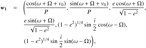 (1)where P is the orbital period and v0 is the true anomaly at a reference epoch (typically that of a specific data point of a time close to periastron passage). This choice was dictated by the following considerations:
-
As pointed out in Chauvinet al. (2012), there is a degeneracyin orbital solutions concerning parameters Ω and ω when considering imaged companions. Taking one potential solution with (Ω,ω) values, the same solution but with (Ω + π,ω + π) exactly, gives the same projected orbital motion. The only way to lift this degeneracy is to have independent information about which side of the projected orbit (or of the associated disk) is on the foreground, or to have radial velocity measurements. Hence taking steps on Ω and ω in MCMC can generate convergence difficulties with chains oscillating between two symmetric families of solutions. To avoid this difficulty, we consider angles ω + Ω and ω−Ω which are unambiguously determined. It is indeed easy to express the projected Keplerian model as a function of these angles only.
-
Whenever i = 0, angles Ω and ω are undefined (and so angle ω−Ω), while Ω + ω is still defined. Hence we take variables ∝sin(i/ 2)cos(ω−Ω) and ∝sin(i/ 2)sin(ω−Ω) to avoid a singularity whenever i → 0.
-
The same applies to eccentricity. When e vanishes, Ω + ω itself is undefined. This is why we consider variables ∝ecos(Ω + ω) and ∝esin(Ω + ω).
-
ω + Ω + v0 is defined even when e = i = 0. This is why we chose it in the remaining variables. But as much as possible, we avoid directly taking steps on angular variables themselves, which can lead to convergence problems with jumps around 2π and similar values. This is why we use cos(ω + Ω + v0) and sin(ω + Ω + v0) in the remaining variables.
As explained by Ford (2006), the assumed priors are taking into account in MH, which multiplies the basic probability by the Jacobian of the transformation from the linear vector (lna,e,sini,Ω,ω,tp) to the parameters vectors. This Jacobian reads  (2)
(2)
3.2. Open orbits and universal variables
The parameter vector w1 (1) is well suited to fit low eccentricity orbits. It has nevertheless proved efficient for high eccentricity orbits as well (Beust et al. 2014). Ford (2006) also gives alternate sets of parameters for such orbits. However, none of them can handle open orbits. Moreover, the validity of the fit close to the boundary e = 1 is questionable. Our goal is to allow MCMC-fitting to account for bound or unbound orbits in a continuous manner as well. Some of the variables in Eqs. (1), such as the orbital period P and  are clearly inappropriate and need to be changed. The periastron q is conversely always defined for any type of orbit. So changing P to q and eliminating in Eqs. (1) could be a first solution. We designed a code based on this idea, which turned out not to be efficient. Convergence of Markov Chains could not be reached after billions of iterations. The reason lies in the assumed Keplerian model. To be able to compute the position and velocity of an orbiting companion at a given time (and subsequently a χ2), one needs to solve Kepler’s equation for the eccentric anomaly u as a function of the time t. Kepler’s equation depends on the type of orbit. For an elliptical, parabolic and hyperbolic orbit, this equation reads
  (3)respectively. In the parabolic case, this equation is called Barker’s equation, and u = tan(v/ 2), where v is the true anomaly. M = n(t−tp) is the mean anomaly, while n is the mean motion. This equation holds in all cases, but n is defined as
  in the elliptic and hyperbolic case, and as
  in the parabolic case, where μ = GM is the dynamical mass (M is the central mass). In the random walk process of a Markov chain, permanent switching between these equations lead to instabilities that prevent convergence. A good way to overcome this difficulty is to move to the universal variable formulation (Danby & Burkardt 1983; Burkardt & Danby 1983; Danby 1987), which is a very elegant way to provide a unique and continuous alternative to Kepler’s equation that is valid for any kind of orbit. We first define the energy parameter α as
 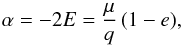 (4)where E is the energy per unit mass. This expression is valid for any orbit. Elliptical orbits are characterised by α> 0, parabolic orbits by α = 0, and hyperbolic ones by α< 0. The eccentric anomaly u is then replaced by the universal variable s. For non-parabolic orbits, s is defined as
  (5)and as
  (6)for parabolic orbits. It can be shown that in any case, we have
 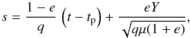 (7)where Y is the y-coordinate in a local OXY referential frame (X axis pointing towards periastron). This shows that the definition of s is continuous, irrespective of the type of orbit. Then, Burkardt & Danby (1983) show that Kepler’s equation can then be rewritten in any case as
 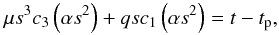 (8)where t is the time, and the ck’s are the Stumpff functions defined as
 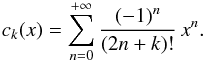 (9)This formulation of Kepler’s equation is valid for any orbit. Using ck(0) = 1 /k !, we see that for α = 0 (parabolic orbit), this equation is equivalent to Barker’s equation. Once this equation is solved for s, the heliocentric distance r and the rectangular coordinates X and Y read
 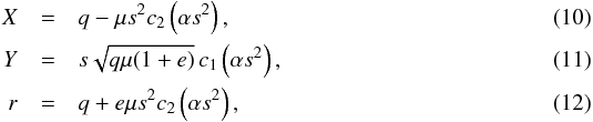 with these formulas applying for any type of orbit. This formalism was used by several authors for specific problems, such as Aarseth (1999) for wide binaries in clusters, or Caballero & Elipe (2001) to solve Keplerian problems with additional disturbing potentials ∝1 /r2. The Kepler advancing routines in the popular symplectic N-body packages Swift (Levison & Duncan 1994) and Mercury (Chambers 1999) are also coded this way for high eccentricity and open orbits. Very recently, Wisdom & Hernandez (2015) have proposed an alternate formalism that avoids the use of Stumpff functions. They claim it to be more efficient. We have not yet tried to apply this and used the Stumpff function theory instead.
Based on the use of Stumpff functions, we designed a new MCMC code, using the following parameter vector:![Mathematical equation: \begin{eqnarray} \vec{w}_2 & = & \left(\rule[-1.5ex]{0pt}{3ex} q\cos(\omega+\Omega), q\sin(\omega+\Omega),\right. \nonumber\\ && \qquad\left.\sin\frac{i}{2}\cos(\omega-\Omega), \sin\frac{i}{2}\sin(\omega-\Omega),e,s_0\right), \label{param2} \end{eqnarray}](/articles/aa/full_html/2016/03/aa27388-15/aa27388-15-eq139.png) (13)where s0 is the universal variable at a given reference epoch. The priors are assumed uniform for Ω, ω, e, and tp, logarithmic for q and ∝sini for i. The Jacobian of the transformation from (lnq,e,sini,Ω,ω,tp) to w2 reads
(13)where s0 is the universal variable at a given reference epoch. The priors are assumed uniform for Ω, ω, e, and tp, logarithmic for q and ∝sini for i. The Jacobian of the transformation from (lnq,e,sini,Ω,ω,tp) to w2 reads  (14)where ds/ dt can be obtained as
 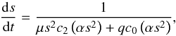 (15)to be evaluated here at s = s0.
3.3. Transformation of angles
This new code was able to reach convergence in the Fomalhaut b case. Convergence, however, appeared hard to reach in the PZ Tel B case. This is due to the structure of the data (Table 2). Indeed, the astrometric data of PZ Tel B reveal a quasi-linear motion that is nearly aligned with the central star. PZ Tel B’s orbit appears extremely eccentric, perhaps unbound, but with a periastron much smaller (≲1 AU) than the measured projected distances. In this context, the local reference frame OXYZ may not be well defined. Only the line of apsides OX is likely to be well constrained by the data, while the two other directions require another, nearly arbitrary angular variable to be fixed. The very bad constraint on that angular variable results into degeneracies in the constraints on angles (Ω,ω,i), which are sufficient to prevent convergence. It thus appears necessary to isolate the badly constrained angular variable into a specific variable. This require us to change the parameter vector w2 (Eq. (13)).
With respect to the sky reference frame (x-axis pointing towards north, y-axis towards east, and z-axis towards the Earth), the basis vectors (eX,eY,eZ) of the local OXYZ reference frame read 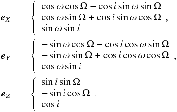 (16)According to our analysis, in the case of PZ Tel B, only eX is well constrained by the data. This results in complex combined constraints on Ω, ω, and i. For instance, if eZ was well constrained by the data, then ω would be the weakly constrained parameter, since eZ is only function of Ω and i. The idea, therefore, is to define new angles in a similar way as in Eq. (16), but in such a way that eX depends on only two angles. We thus introduce new angles i′, Ω′, and ω′ designed in such a way that eX is defined with respect to (i′,Ω′,ω′) in the same manner as eZ is defined with respect to (i,Ω,ω). Similarly eY will be defined like eX, and eZ like eY. We thus write
 ![Mathematical equation: \begin{eqnarray} \vec{e}_X&&\left\{ \begin{array}{l} \sin i'\sin\Omega'\\[\jot] -\sin i'\cos\Omega'\\[\jot] \cos i' \end{array}\right.\!\!,\nonumber\\[2mm] \vec{e}_Y&&\left\{ \begin{array}{l} \cos\omega'\cos\Omega'-\cos i'\sin\omega'\sin\Omega' \\[2mm] \cos\omega'\sin\Omega'+\cos i'\sin\omega'\cos\Omega' \\[2mm] \sin'\omega\sin i' \end{array}\right.\!\!,\nonumber\\[2mm] \vec{e}_Z&&\left\{ \begin{array}{l} -\sin\omega'\cos\Omega'-\cos i'\cos\omega'\sin\Omega'\\[2mm] -\sin\omega'\sin\Omega'+\cos i'\cos\omega'\cos\Omega'\\[2mm] \cos\omega'\sin i' \end{array}\right.\!\!. \label{exeyez2} \end{eqnarray}](/articles/aa/full_html/2016/03/aa27388-15/aa27388-15-eq164.png) (17)The comparison between formulas (16) and (17) gives the correspondence between the two sets of angles. Now, the line of apsides is defined by i′ and Ω′ only, and ω′, the badly constrained angular variable, is undefined if q vanishes. It is therefore worth modifying vector w2 according to this transformation. However, one should not forget that vector w2 was designed to avoid the natural degeneracy of astrometric solution between (Ω,ω) and (Ω + π,ω + π). It can be seen from Eqs. (16) and (17) that changing (Ω,ω) to (Ω + π,ω + π) is equivalent to changing (i′,ω′) to (π−i′,−ω′), while leaving Ω′ unchanged. This transformation leaves the first two components of eX and eY unchanged (which explains the degeneracy of the projected orbit), as well as the third component of eZ, while all remaining components are changed to their opposites. The new parameter vector must remain unchanged with this transformation as well, to avoid convergence difficulties. We chose the following new parameter vector:
(17)The comparison between formulas (16) and (17) gives the correspondence between the two sets of angles. Now, the line of apsides is defined by i′ and Ω′ only, and ω′, the badly constrained angular variable, is undefined if q vanishes. It is therefore worth modifying vector w2 according to this transformation. However, one should not forget that vector w2 was designed to avoid the natural degeneracy of astrometric solution between (Ω,ω) and (Ω + π,ω + π). It can be seen from Eqs. (16) and (17) that changing (Ω,ω) to (Ω + π,ω + π) is equivalent to changing (i′,ω′) to (π−i′,−ω′), while leaving Ω′ unchanged. This transformation leaves the first two components of eX and eY unchanged (which explains the degeneracy of the projected orbit), as well as the third component of eZ, while all remaining components are changed to their opposites. The new parameter vector must remain unchanged with this transformation as well, to avoid convergence difficulties. We chose the following new parameter vector: 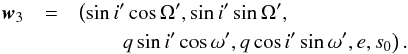 (18)This new vector is invariant in the transformation (i′,ω′)− → (π−i′,−ω′). Its first two components define eX unambiguously. Its third and fourth components vanish when q = 0, i.e. when ω′ is undefined, which avoids singularities. Now, this vector can be expressed as a function of the original angles (i,Ω,ω) directly, so that the formal introduction of the new angles (i′,Ω′,ω′) is unnecessary. The same vector can be written
 ![Mathematical equation: \begin{eqnarray} \vec{w}_3 & = & \left(\rule[-2.5ex]{0pt}{5ex} -\cos\omega\sin\Omega-\sin\omega\cos i\cos\Omega,\right.\nonumber\\ &&\qquad\cos\omega\cos\Omega-\sin\omega\cos i\sin\Omega,\nonumber\\ &&\qquad\qquad\left.q\,\cos i,q\,\frac{\cos\omega\sin\omega\sin^2i} {\sqrt{1-\sin^2i\sin^2\omega}},e,s_0\right). \label{param3b} \end{eqnarray}](/articles/aa/full_html/2016/03/aa27388-15/aa27388-15-eq173.png) (19)It can be checked that this vector is invariant in the transformation (Ω,ω)− → (Ω + π,ω + π). This will be our parameter vector for a second version of the MCMC code. The new Jacobian of the transformation from (lnq,e,sini,Ω,ω,tp) to w3 now reads
(19)It can be checked that this vector is invariant in the transformation (Ω,ω)− → (Ω + π,ω + π). This will be our parameter vector for a second version of the MCMC code. The new Jacobian of the transformation from (lnq,e,sini,Ω,ω,tp) to w3 now reads  (20)This new version succeeded in reaching convergence for PZ Tel B.
3.4. Implementation
The two versions of our code were written in Fortran 90, with an additional OPEN-MP parallel treatment of the computed Markov chains. Our basic strategy is the same is in Beust et al. (2014). We first perform a least-square Levenberg-Marquardt fit of the orbit. This takes only a few seconds to converge towards a local χ2 minimum. Of course, this fit is made by starting with a rought guess of the orbit. The same procedure is reinitiated many times, varying the starting orbit. This allows the variety of local χ2 minima to be probed. Among various minima, a main one, or a series of very similar ones was reached in all the cases described below. This main minimum was selected as a starting point for the MCMC chains. This procedure turns out to speed up the convergence of the chains. This starting point is marked as red bars and black stars in the resulting MCMC posterior plots (see below). We also tried to run the MCMC starting from a random guess instead, and checked that the same posterior distributions were reached, but slower. We also checked in the posterior χ2 distributions that were derived from the runs that, in all cases, the starting point, which was initially derived with Levenberg-Marquardt, actually achieves the best χ2 in the distribution. Strictly speaking, Levenberg-Marquardt works well to quickly derive the best χ2 minimum. This shows that using other least-square fitting algorithms, like downhill simplex for instance, would not lead to a better result, as all these methods aim at finding a χ2 minimum, which is supposed to be the best one. Afterwards, however, MCMC runs reveal that, with sparsely sampled orbits as we are dealing with here, the very best χ2 minimum does not always correspond to a probability peak in the posterior distributions. This intrinsic fact is independent of the method used to get the minimum.
The implementation of the universal variable formalism described above requires an efficient algorithm to compute the Stumpff functions. The series (9) defining them efficiently only converge for sufficiently small x. We use a reduction algorithm described in Danby (1987), which makes use of the following set of formulas: ![Mathematical equation: \begin{eqnarray} c_0(4x)=2\left[c_0(x)\right]^2,& \, & c_1(4x)=c_0(x)c_1(x),\label{qu1}\\ c_2(4x)=\frac{1}{2}\left[c_2(x)\right]^2,&\, & c_3(4x)=\frac{1}{4}c_2(x)+\frac{1}{4}c_0(x)c_3(x).\label{qu2} \end{eqnarray}](/articles/aa/full_html/2016/03/aa27388-15/aa27388-15-eq177.png) Any input argument x is first reduced by successive factors of 4 until it satisfies | x | < 0.1. Then the series up to order 6 are used to get c2(x) and c3(x) only. To compute c0 and c1, the following relations are used:
Any input argument x is first reduced by successive factors of 4 until it satisfies | x | < 0.1. Then the series up to order 6 are used to get c2(x) and c3(x) only. To compute c0 and c1, the following relations are used:  (23)Equations (21) and (22) are then applied recursively to derive the Stumpff functions for the original argument x. Danby (1987) demonstrated the efficiency of this algorithm.
In the fitting routine, the universal Kepler’s Eq. (8) must be solved numerically using a root-finding algorithm. We do it with Newton’s quartic method or with Laguerre-Conway’s method (Danby 1987). To compute the derivatives of the Stumpff function, we use the following relation:  (24)or equivalently, if we define φn(α,s) = sncn(αs2),
  (25)For the special case n = 0, we have
  (26)The same algorithm is implemented in the symplectic N-body integrator Swift (Levison & Duncan 1994) for high eccentricity orbits. Its use turns out to be only a few times (3–4) more consuming of computing time than that of a standard Keplerian formalism, which is based on sine and cosine functions. But it is worth applying this formalism to MCMC the case of very high eccentricity and open orbits, as the use of the universal Kepler’s Eq. (8) eliminates the instabilities because of the permanent switch between the various formulas (3). Thus Markov chains converge more efficiently.
4. Results for Fomalhaut b
Fomalhaut b is known to have a very eccentric orbit, with an eccentricity of ≳0.5, and most probably around 0.8–0.9 (Beust et al. 2014; Pearce et al. 2015). Whether it is actually bound to the central star may be questionable, especially because of the very small coverage fraction of its orbit. If bound, its orbital period is a matter of hundreds of years if not more, while the four available astrometric points span over a period of only eight years. Therefore, as noted by Pearce et al. (2015), what is measured is basically a projected position and a projected velocity onto the sky plane, so that the z-coordinates (i.e. along the line of sight) of the position and velocity are unknown. As a matter of fact, Pearce et al. (2015) use a simple sampling method with these data, which draws random z-coordinates for the position on velocity. They find an eccentricity distribution that is very similar to that derived in Beust et al. (2014) with MCMC. However, in both cases, the orbit was supposed to be bound. The eccentricity distribution of Pearce et al. (2015) nevertheless extends up to e = 1 (that of Beust et al. (2014) stops at e ≃ 0.98), which shows that unbound solutions could exist as well. This justifies the use of our new code to check this possibility.
In its first version (see above), the code was used with the available astrometric data from Kalas et al. (2013) and listed in Beust et al. (2014). Following the prescriptions by Ford (2006), ten chains were run in parallel until the Gelman-Rubin parameters  and
and  repeatedly reach convergence criteria for all parameters in Eq. (13), i.e.
  and
and  . We had already used the same procedure in Chauvin et al. (2012) and Beust et al. (2014). In Beust et al. (2014), these convergence criteria were reached after 6.2 × 10⁷ steps. Here it took 4.25 × 10⁸ steps with the universal variable code, running on the same data. This illustrates how the possibility for Markov chains to extend in the unbound orbit domain increases the complexity of the problem. We also had to fix an arbitrary upper limit emax = 4 for the eccentricity to ensure convergence. Setting larger emax values results in more steps being needed to reach convergence, but the assumed emax = 4 upper limit has some physical justification. A large eccentricity means that Fomalhaut b is an object passing by that is currently encountering a flyby in the Fomalhaut system. The eccentricity of a flyby orbit cannot be arbitrarily large. For a hyperbolic orbit, the eccentricity is directly linked to the relative velocity at infinity v∞ by the energy balance equation
  (27)An upper limit to v∞ can be given by considering a typical dispersion velocity in the solar neighborhood, i.e. ~20 km s-1. Assuming q = 25 AU, i.e. the most probable value for hyperbolic orbits in our distribution (see Fig. 1), this immediately translates into an estimate of an upper limit for the eccentricity emax ≃ 4.
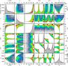 |
Fig. 1 Resulting MCMC posterior distribution of the six orbital elements (q, e, i, Ω, ω, tp) of Fomalhaut b’s orbit, using the universal variable code. The diagonal diagrams show mono-dimensional probability distributions of the individual elements. The off-diagonal plots show bi-dimensional probability maps for the various couples of parameters. This illustrates the correlation between orbital elements. The logarithmic colour scale in these plots is linked to the relative local density of orbital solutions. This is indicated to the side of Fig. 2. In the diagonal histograms, the red bar indicates the location of the best χ2 solution obtained via standard least-square fitting. The location of this solution is marked with black stars in the off-diagonal plots. |
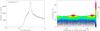 |
Fig. 2 Enlargement of eccentricity histogram (left) and density maps in (Ω,i) space (right) out of Fig. 1. The colour scale appearing on the right side of the right plot map holds for all similar plots in Fig. 1. The eccentricity histogram is the same as in Fig. 1, except that is was truncated at e = 1.5 to allow a better comparison with Beust et al. (2014). In the Ω–i plot, the open star shows the estimated location of the disk plane (Kalas et al. 2005), and the black star indicates the location of the best χ2 solution. |
The global statistics of the posterior orbital distribution obtained from the run is shown in Fig. 1, where distribution histograms for all individual elements (q, e, i, Ω, ω, tp) as well as density maps for all combinations of them are represented. Special enlargements of the plots concerning e and Ω are shown in Fig. 2. In all histogram (mono-dimensional) plots, the red vertical bar that is superimposed on to the plot shows the corresponding value for the best fit (lowest χ2) orbit, which has been obtained independently via a least-square Levenberg-Marquardt procedure. The same orbital solution is marked with black stars in all off-diagonal density plots, which combines two orbital parameters. As explained above, a least-square fit is initiated prior to launching MCMC. The resulting best-fit model is then used as a starting point for the Markov chains, and posterior χ2 distributions show that this solution actually achieves the minimum of the distribution.
We first compare these plots to the corresponding ones in Beust et al. (2014), where the fit was made over the same data set, but limited to bound orbits only. The first striking fact is that the eccentricity distribution extends now beyond e = 1, well into the unbound regime. As suspected, this shows that unbound orbital solutions for Fomalhaut b do exist. The best fit solution is itself an unbound orbit with e ≃ 1.9. We nevertheless note a strong peak in the distribution at e ≃ 0.94, which appears exactly at the same place as in Beust et al. (2014). This clearly shows that, for such a weakly constrained problem, MCMC is definitely superior to least-square.
In fact, the whole eccentricity distribution below e ≲ 0.96 exactly matches the corresponding one in Beust et al. (2014). This shows up in Fig. 2 where the eccentricity histogram was intentionally cut at e = 1.5 to permit a better comparison. First, this validates the present run (as the previous one was done with another code), and second, it shows that the cutoff at e ≃ 0.98 that appeared in the previous distribution, was not physical but rather due to the intrinsic limitation of the code used. The tail of the distribution extends now in the unbound regime up to the emax = 4 limitation that was fixed in the run. The shape of this tail can be fitted as with a e− 3 / 2 power law. We also note (Fig. 1) that the periastron distribution closely matches that of Beust et al. (2014), while extending further out towards larger values. This is clearly due to the contribution of unbound orbits, as can be seen in the q–e probability map.
From this we can derive an estimate of the probability for Fomalhaut b’s orbit being bound, by just counting the number of bound orbits in the whole set. We find pbound = 0.23. This probability actually depends on the assumed limitation emax = 4. If we had let the eccentricity take larger values, the number of unbound orbits in the whole set would have been larger, and subsequently pbound would have been smaller. It is, nevertheless, possible to estimate the ultimate pbound value that would be derived if we put no upper limit on the eccentricity. Taking into account the fact that the tail of the posterior eccentricity distribution roughly falls off as e− 3 / 2, we can extrapolate the distribution up to infinity, integrate it and reintroduce the missing orbits corresponding to e> 4 into the distribution. Our posterior sample of orbits contains 106 solutions. Extrapolating the distribution, we can estimate that ~2.1 × 10⁵, which corresponds to e> 4, are missing in our sample. This changes our probability estimate to pbound = 0.19, which can be considered as a minimum value. However, as the emax = 4 threshold results from a physical consideration (see above), the first derived pbound value can be regarded as robust. This is not very much above the minimum value, which shows that the contribution of very high eccentricity solutions is minor.
This probability is however onl derived from a purely mathematical analysis without any consideration of likelihood. Flybys are rare but not necessarily improbable (see example in Reche et al. 2009). Looking now at the distribution of the other orbital elements, we see in Fig. 2 that the location of the orbit in (Ω,i) still closely matches that of the observed dust disk (the white star in the plot; Kalas et al. 2005), as in Beust et al. (2014). In other words, there is still a strong likelihood of near-coplanarity between Fomalhaut b and the dust disk. This clearly favours a bound configuration rather than a flyby that would have no reason for being coplanar. Another possibility is that Fomalhaut b is just being ejected from the system today. This last configuration nevertheless appears improbable, regardless to the timescale of the ejection (~1000 yr) compared to the age of the system (440 Myr; Mamajek 2012). To conclude, these plausibility considerations, combined with our pbound ≃ 0.23 estimate and the clear peak of the eccentricity distribution at e = 0.94, enable us to emphasise that Fomalhaut b is probably bound to the central star.
The situation is less clear with the argument of periastron. In the ω–e plot (Fig. 1), we see that, depending on whether e< 1 or e> 1, the solutions exhibit different ω values. In Beust et al. (2014), we note that the observed dust disk corresponds to ωdisk = −148.9°. This still roughly matches the ω values for bound orbits, i.e. the bound orbits are still apsidally aligned with the disk with a few tens of degrees.
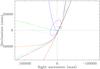 |
Fig. 3 Examples of orbital solutions for Fomalhaut b, in projection onto the sky plane. The star is at the centre of the plot. The black square denotes the location of the observed astrometric points. Various colours are given to the orbits, allowing them to be easily distinguishable from each other. |
The distribution of the time of periastron passage (tp) is similar to that of Beust et al. (2014), except that here we have an additional tail after 1950 that corresponds to unbound orbits. Figure 3 finally shows a few orbital solutions in projection onto the sky plane, with bound and unbound configurations. We note that all solutions fit the observed positions, while assuming very different shapes. We clearly see here the effect of the bad observational orbital coverage.
5. PZ Tel B
5.1. Results
Summary of astrometric positions of PZ Tel B relative to PZ Tel as observed in recent years.
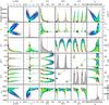 |
Fig. 4 Resulting MCMC posterior distribution of the six orbital elements (q, e, i, Ω, ω, tp) of PZ Tel B’s orbit using the universal variable code, presented in the same manner as for Fomalhaut b in Fig. 1. The plotting conventions are identical. |
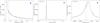 |
Fig. 5 Enlargement of histograms and density maps out of Fig. 4 for the periastron (q) and eccentricity (e) parameters. With respect to Fig. 4, the periastron plot (left) was truncated at q = 1 AU to make the peak at q = 0.07 appear. The right plot is a special zoom of the eccentricity distribution around e = 1. |
As mentioned above, orbital solutions for PZ Tel B (Biller et al. 2010; Mugrauer et al. 2012; Ginski et al. 2014) all yield very eccentric orbits (e> 0.6). These orbital determinations were performed assuming a bound orbit, so that no test at e ≥ 1 was done. This assumption is, however, questionable given the orbital solutions found. We thus ran our universal variable MCMC code with the available astrometric data of PZ Tel B (Table 2). As explained above (Sect. 2), we used the second version of the code with parameter vector w3 (Eq. (19)), which ensures a better convergence.
Even in this case, convergence was hard to reach. Ten chains were run in parallel. After 1.5 × 10¹⁰ steps, the Gelman-Rubin parameter values for the six variables in w3 range from between 1.006 and 1.019, while the parameter values range from between 260 and 800. The run was stopped there to save computing time, since reaching the demanded criteria ( and for all variables) would have demanded many more steps. The and values reached at the stopping point must nevertheless be considered as characteristic for an already very good convergence, so that we can trust the resulting posterior distribution. We checked indeed that the alternate posterior distributions that we were able to derive by stopping the computation earlier, i.e. at a point when the and values were somewhat further away from convergence criteria, did not present significant differences to those presented below. Noticeably, nothing comparable in terms of convergence criteria was reached using the first version of the code that uses parameter vector w2 (Eq. (13)).
The global statistics of the posterior orbital distribution obtained from the run is shown in Fig. 4, which was built with the same plotting conventions as Fig. 1 for Fomalhaut b. In particular, the red bar and the black star indicate the best-fit orbit obtained via Levenberg-Marquardt. Special enlargements concerning the periastron and the eccentricity are shown in Fig. 5.
The most striking feature that shows up is the eccentricity distribution. As expected, PZ Tel B’s orbit appears extremely eccentric, but the eccentricity distribution is drastically different from that of Fomalhaut b. As pointed out by Pearce et al. (2015), the temporal coverage of Fomalhaut b’s orbit is so small that what is measured is basically a projected position and a projected velocity, with no information about position and velocity along the line of sight. Consequently, solutions with arbitrarily high eccentricities are mathematically possible. This is not the case for PZ Tel B. Table 2 shows that the motion followed over five years is quasilinear, but with a separation with the central star that increased by more than 60%. Even if the orbital coverage is still small (see Fig. 6), this is more than just a projected position and project velocity measurement. Consequently, no tail extending to arbitrarily large values is obtained with MCMC. All solutions naturally concentrate in the range 0.91 <e< 1.23. The eccentricity distribution appears extremely concentrated around e = 1. The enlargement in Fig. 5 that is close to e = 1 reveals a peak near e = 1.00. The median of the distribution is at e = 1.001275; 67% and 95% confidence levels are 0.965 <e< 1.024 and 0.906 <e< 1.157, respectively. We compare the eccentricity distribution to that recently found by Ginski et al. (2014), who derived 0.622 <e< 0.9991 using a least-squares Monte-Carlo (LSMC) approach, but restricted to bound orbits. Of course our distribution now extends beyond e = 1, but our lower bound (e = 0.91) is significantly larger than theirs. This is due to our additional data points rather than to the method used.
The periastron distribution shows a sharp peak around q = 0.07 AU. The q–e map (Fig. 4) actually reveals two branches of solutions, one with a bound solution and one with unbound solutions. But most solutions concentrate close to e = 1 and q = 0.07 AU. The inclination shows a peak at i = 98°. This corresponds to a nearly edge-on configuration and could explain the quasilinear motion. But solutions up to i = 150° are also possible. The i–e map shows that the larger inclination solutions actually correspond to those with e ≃ 1. All solutions have i> 90°, showing that the orbit is viewed in a retrograde configuration from the Earth. The distribution of the time of periastron (tp) exhibits a very sharp peak in 2002.5 that also corresponds to orbits with e ≃ 1.
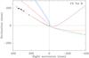 |
Fig. 6 Examples of orbital solutions for PZ Tel B, in projection onto the sky plane. The star is at the centre of the plot. The data points appear in the upper left corner of the plot. As in Fig. 3, colours are given to individual orbits to allow them to be distinguished from each other. |
Figure 6 shows several orbital solutions in projection onto the sky plane. We see that the solutions actually fit the data points, but they all have a much smaller periastron. Figure 7 shows the best χ2 orbit in a similar way, but superimposed on to a density map that shows the predicted projected positions as of July 22, 2003 (2003.556). Indeed, Masciadri et al. (2005) report a non-detection of PZ Tel B in a NACO image from that day. They conclude that no giant planet was present at a separation larger than 170 mas from the star. In Fig. 7, according to our extrapolation we see that, at the corresponding epoch, PZ Tel B was much closer to the star. In most cases, this was shortly after periastron but, in any case, it was closer to the star than 170 mas. Our extrapolation is therefore in agreement with the non-detection by Masciadri et al. (2005).
5.2. Discussion
The exact nature of PZ Tel B’s orbit around PZ Tel is still controversial. Our orbital analysis shows that both bound or unbound solutions are valid, but that the eccentricity distribution is strongly peaked around e = 1. If PZ Tel B is unbound to PZ Tel, it could be a passing-by object (a flyby). This is hard to believe, given the very small periastron value, and also considering the fact that both the star and the companion seem to be young objects (Schmidt et al. 2014). This cannot however be ruled out mathematically. From Eq. (27) with M = 1.25 M⊙ and v∞ = 20 km s-1, we derive e = 1.012 for q = 0.07 AU and e = 1.181 for q = 1 AU, which is still in the tail of the eccentricity distribution, although not in the main peak. We nevertheless think this possibility is very unlikely.
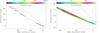 |
Fig. 7 Density map of extrapolated projected position of PZ Tel B on July 22, 2003, superimposed to the best χ2 orbit. Left plot: large scale map showing the data points, the orbit, the predicted position for that orbit on 2016.0, 2018.0, 2010.0 (blue points), and the cloud of positions on July 22, 2003, computed for all solutions out of our posterior sample (shortly after periastron); right plot: enlargement of the periastron region with the cloud of projected positions. The peak of the distribution is indicated with a black star. |
Still if PZ Tel B is unbound, it could be an escaping companion that was recently ejected by some gravitational perturbation. Two problems arise with this hypothesis. First, the ejection must have occurred very recently (a few years ago). Given the age of the star (23 Myr, Mamajek & Bell 2014; Binks & Jeffries 2014; Malo et al. 2014), the probability of witnessing such an event today is very low, about ~10-6 if we consider the timescale of the ejection (~10 yr) and the fact that this type of ejection should not occur more than a few times in the history of the system. Second, to efficiently perturb a 40 MJup companion, an additional object of comparable mass (at least) is required. As of yet, no such additional companion has been detected.
So, PZ Tel B is presumably a bound companion. If so, one must explain its extremely high eccentricity. It could be the result of secular perturbation processes such as the Kozai-Lidov mechanism (Kozai 1962; Krymolowski & Mazeh 1999; Ford et al. 2000). This is a likely mechanism for generating very high eccentricities. But here again, given the fairly high mass of PZ Tel B, this would require a more massive outer companion that should probably have already been discovered.
6. Hidden inner companions?
6.1. Fomalhaut b
Pearce et al. (2014) argue that imaged substellar companions that appear very eccentric with a first order orbital fit could actually be much less eccentric due to the presence of an unseen inner companion. The reason is that the measured astrometry is necessarily relative to the central star while, in the presence of a massive enough inner companion, the Keplerian motion of the imaged body should be considered around the centre of mass of the system. Pearce et al. (2014) develop a fully analytical study showing how the presence of such an unseen companion could artificially enhance the fitted eccentricity.
Pearce et al. (2014) present a detailed study dedicated to the case of Fomalhaut b, concluding that in any case, Fomalhaut b must be significantly eccentric. According to them, in the best realistic configuration, a ~12 MJup companion orbiting Fomalhaut at 10 AU could account for an ~10% overestimate of Fomalhaut b’s orbital eccentricity. This would, for instance, shift the eccentricity peak from e = 0.94 to e = 0.85. This possibility cannot be ruled out until the inner configuration of Fomalhaut’s planetary system remains unconstrained. It would also be compatible with the scenario outlined by Faramaz et al. (2015) to explain the origin of Fomalhaut b’s eccentricity. According to this model, Fomalhaut b should have formerly resided at ~60 AU in the 5:2 mean-motion resonance with another Jupiter-sized planet (termed Fomalhaut c) located at ~100 AU. Then, because of the resonant action, its eccentricity would have increased, and it would have been ejected towards its present-day orbit. This is still compatible with the hypothetical presence of another massive planet orbiting inside at 10 AU. The only difficulty is that, with e = 0.85, Fomalhaut b’s periastron is still as low as ~18 AU, which is still close enough to 10 AU to raise the question of its orbital stability versus perturbations by the hidden companion. However, according to Faramaz et al. (2015)’s scenario, Fomalhaut b’s orbit must today already cross that of the putative Fomalhaut c planet orbiting at 100 AU. So in any case, Fomalhaut b must today lie on a metastable orbit. Adding another massive body deep inside the system does not change this conclusion. Consequently, the presence of an additional massive planet orbiting Fomalhaut at 10 AU that would artificially enhance Fomalhaut b’s eccentricity by ~10% cannot be ruled out, as being still compatible with all observational constraints. Moreover it does not affect the dynamical scenario of Faramaz et al. (2015).
6.2. PZ Tel B
The case of PZ Tel B is more complex. The main difference with Fomalhaut b is that it is imaged over a more significant part of its orbit. As noted by Pearce et al. (2015), the detected astrometric motion of Fomalhaut b is basically compatible with a straight line at constant speed, so that what is measured is not much more than a projected position and a projected velocity. This is not the case for PZ Tel B, as the projected distance to the star is already able to vary significantly over the observation period (Table 2). This is actually the reason why the fitted eccentricity distribution does not extend towards arbitrarily large values (Fig. 5). Consequently, an analytical study of the potential effect of an unseen companion on the fitted orbit is less easy. Pearce et al. (2014) nevertheless calculate that a companion, at least as massive as 130 MJup orbiting PZ Tel at 5.5 AU is required to mimic PZ Tel B’s eccentricity. But recent imaging by Ginski et al. (2014) exclude companions more massive than 26 MJup at this distance.
However, as for Fomalhaut b, an unseen companion could account only partially for PZ Tel B’s eccentricity. We decided to perform an automated search based on this idea. Our strategy is the following: We arbitrarily fix the characteristics of an unseen companion (mass and orbit) that we may call it PZ Tel c. Given these characteristics, we calculate at each time the expected position of the centre of mass of the system and recompute the astrometric positions of PZ Tel B relative to this centre of mass. Then we restart a least-square fit and check the eccentricity of the best χ2 solution obtained. This process is then automatically reinitiated many times, changing the characteristics of PZ Tel c until a solution that yields a least-square fit with the minimal eccentricity is found. Of course we make several attempts, varying the starting points. These showed that, in any case, PZ Tel B’s eccentricity of the best χ2 solution never goes below ~0.7.
For the most favourable configuration, the MCMC fit is re-launched to derive the statistical distributions of orbits. We present here one of these runs.
Characteristics of a putative PZ Tel c that leads to a less eccentric solution for PZ Tel B.
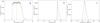 |
Fig. 8 Resulting MCMC posterior distribution of the periastron q (left), the eccentricity e (middle), and the inclination i (right) of PZ Tel B’s orbit using the universal variable code, which is based on the modified data from Table 4. The plotting conventions are the same as in Fig. 5. |
The characteristics of the putative PZ Tel c that correspond to this run are listed in Table 3 and the recomputed barycentric astrometry of PZ Tel B is given in Table 4. The main characteristics of the result of the run (histograms of periastron, eccentricity, and inclination) are shown in Fig. 8. The first thing we note is that the putative PZ Tel c companion (12 MJup at 3.5 AU) is compatible with the current non-detection limits (Ginski et al. 2014). Second, the difference between the computed barycentric astrometric data and the measured data is small, often within the error bars of Table 2. Nonetheless, the difference in the orbital fit (Fig. 8) is striking. PZ Tel B still appears eccentric, but its eccentricity is now confined to between 0.65 and 0.8, the best χ2 orbit (the red bar in the plots) having e ≃ 0.68. According to this analysis, PZ Tel B would clearly be a bound companion. Its periastron q ranges from between 8 and 24 AU, but all orbits with q< 8 AU have been eliminated in the fitting procedure as being, presumably, highly unstable versus gravitational perturbations from the hypothetical PZ Tel ccompanion. Letting the periastron distribution extend towards lower values would generate solutions with larger eccentricities, but these would probably not be physical.
6.3. Dynamical analysis
Figure 8 also reveals that PZ Tel B’s orbital inclination is very close to 90°, meaning an almost edge-on viewed orbit. Simultaneously, PZ Tel c’s inclination appears extremely low (Table 3), meaning a pole-on orbit. This allows us to question the dynamical stability of such a system. According to our fit, PZ Tel B’s periastron is most probably around ~10 AU, which is ~3 times larger than the semi-major axis of PZ Tel c’s semi-major axis. This is, in principle, marginally enough to ensure the dynamical stability of the whole. But here both orbits are nearly perpendicular. In this context, the inner orbit is likely to be trapped in the Kozai-Lidov mechanism (Kozai 1962; Krymolowski & Mazeh 1999; Ford et al. 2000) that is characterised by huge eccentricity changes. This could trigger orbital instability.
 |
Fig. 9 Orbital evolution of the PZ Tel B+c system, as computed with pure Newtonian dynamics over 106yr, using HJS integrator. Left: eccentricities of both orbits; red is for PZ Tel c and green for PZ Tel B; middle: mutual inclination between both orbital planes; right: periastron of PZ Tel c, in logarithmic scale |
We thus decided to numerically investigate the dynamical stability of this three body system, starting from the best χ2 solution for PZ Tel B, in Fig. 8, and with the orbital solution from Table 3. As the fitted orbit of PZ Tel B is barycentric, we used our HJS symplectic code (Beust 2003) that naturally works in Jacobi coordinates, which is the case here. The result is presented in Fig. 9, which shows the orbital evolution of the system over 106 yr. The regular evolution pattern is an indication of stability. In fact, the integration was carried out up to 107 yr, which reveals the same behaviour as in the first 106yr. Moreover, the semi-major axes of both planets (not shown here) appeared to be remarkably stable, which confirms the stability. Nonetheless, PZ Tel c’s eccentricity exhibits large amplitude oscillations coupled with oscillation of the mutual inclination between both orbital planes. This behaviour is characteristic of a strong Kozai resonance. We note, however, that in high eccentricity phases, the mutual inclination does not drop down to 0 but up towards 180° (retrograde orbits). This is thus an example of retrograde Kozai resonance.
This picture is however very probably erroneous. In fact, given the almost perfectly perpendicular initial configuration of the orbits, the Kozai cycles drive PZ Tel c up to very high eccentricity values. The peak eccentricity in the cycles is actually close to ~0.998. Considering that PZ Tel c’s semi-major axis is nearly constant, its periastron must drop down to very small values during peak eccentricity phases. The right plot of Fig. 9 confirms this fact. The minimum periastron value in the peaks ranges between 104AU and 10-3AU. With a mass of 1.25 M⊙, PZ Tel’s radius can be estimated at 9 × 10⁵km, i.e., 6 × 10⁻³AU. PZ Tel c is thus, potentially, subject to collision with the central star. However, when the periastron decreases in high eccentricity phases, PZ Tel c is very probably affected by tides from the central star that may prevent physical collisions. Tides were not taken into account in the run described in Fig. 9, so that this picture does not hold.
 |
Fig. 10 Orbital evolution of the PZ Tel c system in a similar configuration as in Fig. 9 with respect to PZ Tel B, but with tides taken into account, assuming Q = 105 quality factor. The computation was made using the HJS integrator to which tides and post-Newtonian corrections were added. Left: semi-major axis; middle: eccentricity; right: mutual inclination between both orbital planes |
We thus recomputed the secular evolution of the same three-body system, but now taking tides between the central star and PZ Tel c into account. The computation was done using a special version of the HJS integrator, to which we added tides and relativistic post-Newtonian corrections. The details of this code are presented in Beust et al. (2012) with an application to the GJ 436 system. Tides mainly depend on the assumed tidal dissipation parameter Qp for the planet, a dimensionless parameter that is related to the rate of energy dissipated through tides per orbital period (Barker & Ogilvie 2009). The smaller the Qp, the more efficient the tidal dissipation is. Qp is very hard to estimate, but typical values for giant planets range around 105 within one order or magnitude (Zhang & Hamilton 2008).
Figure 10 shows the result of this kind of simulation, assuming Qp = 105 for PZ Tel c. The difference with the previous run is striking. PZ Tel c’s semi-major axis appears to remain constant for ~3 × 10⁴ yr, and to suddenly drop thereafter. During the first phase (before 3 × 10⁴yr), the eccentricity gradually increases before decreasing, and the mutual inclination decreases before stabilising. The explanation is as follows: in the first phase, the periastron remains too large to allow tides to be active. But the Kozai mechanism causes an eccentricity increase until a point where tides act at periastron. The subsequent energy dissipation then causes a rapid decay of PZ Tel c’s orbit and a subsequent circularisation. This scenario is actually similar to the one depicted in Beust et al. (2012) for GJ 436 and by Fabrycky & Tremaine (2007). In the latter cases, several Kozai-Lidov oscillations, together with tidal friction, first occur before the inner orbit starts to decay. Here this state is reached at the very first eccentricity peak, thanks to very strong tides when the periastron gets very close to the stellar surface.
The consequence is that tides prevent the deduced orbital configuration between PZ Tel B and PZ Tel c from being stable, since the hypothetical PZ Tel c inevitably migrates to a much closer orbit after only 3 × 10⁴yr. This result obviously depends on the assumed Qp value. We thus tried other runs with increased Qp values (106 and above) to reduce the strength of tides. This appeared to only delay the time of the orbital decay without changing the basic scenario. In any case, PZ Tel c ends up on a tight orbit (<0.1 AU), on a timescale in any case much lower than the age of the system.
Our conclusion is that the PZ Tel c scenario that is depicted here to account for the apparent very high eccentricity of PZ Tel B does not hold, since it would require an orbital configuration that cannot be stable. We are thus back to our conclusion that PZ Tel B’s orbit is really very close to a parabolic state, as deduced from our initial MCMC analysis.
7. Conclusion
We have developed a new MCMC code based on the use of universal Keplerian variables, which is dedicated to the orbital fit of imaged companions with very high eccentricities or unbound orbits. This code was successfully applied to the specific cases of Fomalhaut b and PZ Tel B. As far as Fomalhaut b is concerned, we confirm our orbital determination of Beust et al. (2014), but we show that the eccentricity distribution can extend above e = 1 in the unbound regime. This is in agreement with the analysis of Pearce et al. (2015) who show that, for companions that are imaged over a very small orbital arc, the unknown radial velocity renders unbound orbits possible. We, however, think that Fomalhaut b is very probably a bound companion, although very eccentric. The case of PZ Tel B is more complex. Our code reveals a very different eccentricity distribution than for Fomalhaut b. Indeed, PZ Tel B’s eccentric distribution exhibits a very sharp peak around e = 1.
According to Pearce et al. (2014), imaged companions can appear much more eccentric than they are actually, thanks to the presence of hidden inner companions that affect that astrometric data. Pearce et al. (2014) have already shown that this model cannot account for Fomalhaut b’s eccentricity. For PZ Tel B, we show that a hidden ~12MJup companion orbiting at ~3.5 AU in a pole-on configuration (contrary to the edge-on orbit of PZ Tel B) could mimic an almost unbound orbit despite a real eccentricity around ~0.7. However, because of the combination of tides and a Kozai-Lidov mechanism, this configuration is dynamically unstable. We are thus back to the conclusion that PZ Tel B has very high eccentricity and is a possible unbound companion.
The dynamical origin of Fomalhaut b and its configuration relative to the dust disk that orbits Fomalhaut was recently investigated by Faramaz et al. (2015). According to this model, the Fomalhaut system should harbour another, more massive planet that controls the shape of the disk. Fomalhaut b could have formerly resided in a mean-motion resonance with that planet, and could have been put on its present day eccentricity via a gradual eccentricity increase and one or several close encounters. The case of PZ Tel B is more complex. According to our orbital determination, its eccentricity is, in any case, very close to 1 if not above. The planet passed through a very close (<0.1 AU) periastron in 2002, consistent with its non-detection in 2003 NaCo images (Masciadri et al. 2005). Highly eccentric orbits with very small periastron are usually triggered by a Kozai-Lidov mechanism or by mean-motion resonance with a moderately eccentric outer companion (such as, in the so-called Falling Evaporating Body scenario in the βPictoris system Beust & Morbidelli 2000). But, given the estimated mass of PZ Tel B, this would require a perturbing companion in the low stellar mass regime. This kind of companion would have already been detected. Apart from a very peculiar past encounter event, there is therefore no obvious explanation for the unusual orbital configuration of PZ Tel B. Further monitoring of this system will increase our understanding of it.
Acknowledgments
Most of the computations presented in this paper were performed using the Froggy platform of the CIMENT infrastructure (https://ciment.ujf-grenoble.fr), which is supported by the Rhône-Alpes region (GRANT CPER07_13 CIRA), the OSUG@2020 labex (reference ANR10 LABX56) and the Equip@Meso project (reference ANR-10-EQPX-29-01) of the programme Investissements d’Avenir, supervised by the Agence Nationale pour la Recherche. The MCMC code used in this paper can be obtained freely upon request to This email address is being protected from spambots. You need JavaScript enabled to view it. .
References
- Aarseth, S. J. 1999, Celest. Mech., 73, 127 [NASA ADS] [CrossRef] [Google Scholar]
- Barker, A. J., & Ogilvie, G. I. 2009, MNRAS, 395, 2268 [NASA ADS] [CrossRef] [Google Scholar]
- Bell, C. P. M., Mamajek, E. E., & Naylor, T. 2015, MNRAS, 454, 593 [NASA ADS] [CrossRef] [Google Scholar]
- Beust, H. 2003, A&A, 400, 1129 [NASA ADS] [CrossRef] [EDP Sciences] [Google Scholar]
- Beust, H., & Morbidelli, A. 2000, Icarus, 143, 170 [NASA ADS] [CrossRef] [Google Scholar]
- Beust, H., Bonfils, X., Montagnier, G., Delfosse, X., & Forveille, T. 2012, A&A, 545, A88 [NASA ADS] [CrossRef] [EDP Sciences] [Google Scholar]
- Beust, H., Augereau, J.-C., Bonsor, A., et al. 2014, A&A, 561, A43 [NASA ADS] [CrossRef] [EDP Sciences] [Google Scholar]
- Biller, B. A., Liu, M. C., Wahhaj, Z., et al. 2013a, ApJ, 720, L82 [Google Scholar]
- Biller, B. A., Liu, M. C., Wahhaj, Z., et al. 2013b, ApJ, 777, 160 [NASA ADS] [CrossRef] [Google Scholar]
- Binks, A. S., & Jeffries, R. D. 2014, MNRAS, 438, L11 [NASA ADS] [CrossRef] [Google Scholar]
- Bonnefoy, M., Lagrange, A.-M., Boccaletti, A., et al. 2011, A&A, 528, L15 [NASA ADS] [CrossRef] [EDP Sciences] [Google Scholar]
- Bonnefoy, M., Marleau, G.-D., Galicher, R., et al., 2014, A&A, 567, L9 [NASA ADS] [CrossRef] [EDP Sciences] [Google Scholar]
- Burkardt, T. M., & Danby, J. M. A. 1983, Celest. Mech., 31, 317 [NASA ADS] [CrossRef] [Google Scholar]
- Caballero, J. A., & Elipe, A. 2001, Astron. Astrophys. Transactions, 19, 869 [NASA ADS] [CrossRef] [Google Scholar]
- Chambers, J. E. 1999, MNRAS, 304, 793 [NASA ADS] [CrossRef] [MathSciNet] [Google Scholar]
- Chauvin, G., Lagrange, A.-M., Beust, H., et al. 2012, A&A, 542, A41 [NASA ADS] [CrossRef] [EDP Sciences] [Google Scholar]
- Currie, T., Debes, J., & Rodigas, T. J. 2012, ApJ, 760, L32 [NASA ADS] [CrossRef] [Google Scholar]
- Danby, J. M. A. 1987, Celest. Mech., 40, 303 [NASA ADS] [CrossRef] [Google Scholar]
- Danby, J. M. A., & Burkardt, T. M. 1983, Celest. Mech., 31, 95 [NASA ADS] [CrossRef] [Google Scholar]
- Devillard, N. 1997, The Messenger, 87, 19 [NASA ADS] [Google Scholar]
- Fabrycky, D., & Tremaine, S. 2007, ApJ, 669, 1298 [NASA ADS] [CrossRef] [Google Scholar]
- Faramaz, V., Beust, H., Augereau, J.-C., Kalas, P., & Graham, J. R. 2005, A&A, 573, A87 [NASA ADS] [CrossRef] [EDP Sciences] [Google Scholar]
- Ford, E. B. 2005, AJ, 129, 1706 [Google Scholar]
- Ford, E. B. 2006, ApJ, 642, 505 [NASA ADS] [CrossRef] [Google Scholar]
- Ford, E. B., Kozinsky, B., & Rasio, F. A. 2000, ApJ, 535, 385 [NASA ADS] [CrossRef] [Google Scholar]
- Galicher, R., Marois, C., Zuckerman, B., & Macintosh, B. 2013, ApJ, 769, 42 [Google Scholar]
- Ginski, C., Schmidt, T. O. B., Mugrauer, M., et al. 2014, MNRAS, 444, 2280 [NASA ADS] [CrossRef] [Google Scholar]
- Janson, M., Carson, J. C., Lafrenière, D., et al. 2012, ApJ, 747, 116 [NASA ADS] [CrossRef] [Google Scholar]
- Kalas, P., Graham, J. R., Chiang, E., et al. 2005, Nature, 435, 1067 [NASA ADS] [CrossRef] [PubMed] [Google Scholar]
- Kalas, P., Graham, J. R., Chiang, E., et al. 2008, Science, 322, 1345 [NASA ADS] [CrossRef] [PubMed] [Google Scholar]
- Kalas, P., Graham, J. R., Fitzgerald, M. P., & Clampin, M. 2013, ApJ, 775, 56 [NASA ADS] [CrossRef] [Google Scholar]
- Kennedy, G. M., & Wyatt, M. C. 2011, MNRAS, 412, 2137 [NASA ADS] [CrossRef] [Google Scholar]
- Krymolowski, Y., & Mazeh, T. 1999, MNRAS, 304, 720 [NASA ADS] [CrossRef] [Google Scholar]
- Kozai, Y. 1962, AJ, 67, 591 [Google Scholar]
- Lenzen, R., Hartung, M., Brandner, W., et al. 2003, in Instrument Design and Performance for Optical/Infrared Ground-based Telescopes, Proc. SPIE, eds. M. Iye, & M. Moorwood, 4841, 944 [Google Scholar]
- Levison, H. F., & Duncan, M. J. 1994, Icarus, 108, 18 [NASA ADS] [CrossRef] [Google Scholar]
- McCaughrean, M. J., & Stauffer, J. R. 1994, AJ, 108, 1382 [NASA ADS] [CrossRef] [Google Scholar]
- Malo, L., Doyon, R., Feiden, G. A., et al. 2014, ApJ, 792, 37 [NASA ADS] [CrossRef] [Google Scholar]
- Maire, A.-L., Bonnefoy, M., Ginski, C., et al. 2016, A&A, 587, A56 [NASA ADS] [CrossRef] [EDP Sciences] [Google Scholar]
- Mamajek, E. E. 2012, ApJ, 754, L20 [NASA ADS] [CrossRef] [Google Scholar]
- Mamajek, E. E., & Bell, C. P. M. 2014, MNRAS, 445, 2169 [NASA ADS] [CrossRef] [Google Scholar]
- Marois, C., Lafrenière, D., Doyon, R., Macintosh, B., & Nadeau, D. 2006, A&A, 641, 556 [Google Scholar]
- Masciadri, E., Mundt, R., Henning, T., Alvarez, C., & Barrado y Nevascués, D. 2005, ApJ, 625, 1004 [NASA ADS] [CrossRef] [Google Scholar]
- Messina, S., Desidera, S., Turatto, M., Lanzafame, A. C., & Guinan, E. F. 2010, A&A, 520, A15 [NASA ADS] [CrossRef] [EDP Sciences] [Google Scholar]
- Mugrauer, M., Vogt, N., Neuhäuser, R., & Schmidt, T. O. B. 2010, A&A, 523, L1 [NASA ADS] [CrossRef] [EDP Sciences] [Google Scholar]
- Mugrauer, M., Röll, T., Ginski, C., et al. 2012, MNRAS, 424, 1714 [NASA ADS] [CrossRef] [Google Scholar]
- Nelson, B., Ford, E. B., & Payne, M. J. 2014, ApJS, 210, 11 [NASA ADS] [CrossRef] [Google Scholar]
- Pearce, T. D., Wyatt, M. C., & Kennedy, G. M. 2014, MNRAS, 437, 2686 [NASA ADS] [CrossRef] [Google Scholar]
- Pearce, T. D., Wyatt, M. C., & Kennedy, G. M. 2015, MNRAS, 448, 3679 [NASA ADS] [CrossRef] [Google Scholar]
- Pueyo, L., Soummer, R., Hoffmann, J., et al. 2015, ApJ, 803, 31 [NASA ADS] [CrossRef] [Google Scholar]
- Reche, R., Beust, H., & Augereau, J.-C. 2009, A&A, 493, 661 [NASA ADS] [CrossRef] [EDP Sciences] [Google Scholar]
- Rousset, G., Lacombe, F., Puget, P., et al. 2003, in Adaptive Optical System Technologies II, eds. P.-L. Wizinowich, & D. Bonaccini, Proc. SPIE, 4839, 140 [Google Scholar]
- Soummer, R., Brendan Hagan, J., Pueyo, L., et al. 2011, ApJ, 741, 55 [NASA ADS] [CrossRef] [Google Scholar]
- Spencer Jones, H., & Jackson, J. 1936, Proper motions of stars in the zone catalogue of 20 843 stars 1900 (London: HMSO) [Google Scholar]
- Schmidt, T. O. B., Mugrauer, M., Neuhäuser, R., et al. 2014, A&A, 566, A85 [NASA ADS] [CrossRef] [EDP Sciences] [Google Scholar]
- Torres, C. A. O., Quast, G. R., da Silva, L., et al. 2006, A&A, 460, 695 [NASA ADS] [CrossRef] [EDP Sciences] [Google Scholar]
- van Dessel, E., & Sinachopoulos, D. 1993, A&AS, 100, 517 [NASA ADS] [Google Scholar]
- Wisdom, J., & Hernandez, D. M. 2015, MNRAS, 453, 3015 [NASA ADS] [CrossRef] [Google Scholar]
- Zhang, K., & Hamilton, D. P. 2008, Icarus, 193, 267 [NASA ADS] [CrossRef] [Google Scholar]
- Zuckerman, B., Song, I., Bessell, M. S., & Webb, R. A. 2001, ApJ, 562, L87 [NASA ADS] [CrossRef] [Google Scholar]
All Tables
Summary of astrometric positions of PZ Tel B relative to PZ Tel as observed in recent years.
Characteristics of a putative PZ Tel c that leads to a less eccentric solution for PZ Tel B.
All Figures
|
Fig. 1 Resulting MCMC posterior distribution of the six orbital elements (q, e, i, Ω, ω, tp) of Fomalhaut b’s orbit, using the universal variable code. The diagonal diagrams show mono-dimensional probability distributions of the individual elements. The off-diagonal plots show bi-dimensional probability maps for the various couples of parameters. This illustrates the correlation between orbital elements. The logarithmic colour scale in these plots is linked to the relative local density of orbital solutions. This is indicated to the side of Fig. 2. In the diagonal histograms, the red bar indicates the location of the best χ2 solution obtained via standard least-square fitting. The location of this solution is marked with black stars in the off-diagonal plots. |
| In the text | |
|
Fig. 2 Enlargement of eccentricity histogram (left) and density maps in (Ω,i) space (right) out of Fig. 1. The colour scale appearing on the right side of the right plot map holds for all similar plots in Fig. 1. The eccentricity histogram is the same as in Fig. 1, except that is was truncated at e = 1.5 to allow a better comparison with Beust et al. (2014). In the Ω–i plot, the open star shows the estimated location of the disk plane (Kalas et al. 2005), and the black star indicates the location of the best χ2 solution. |
| In the text | |
|
Fig. 3 Examples of orbital solutions for Fomalhaut b, in projection onto the sky plane. The star is at the centre of the plot. The black square denotes the location of the observed astrometric points. Various colours are given to the orbits, allowing them to be easily distinguishable from each other. |
| In the text | |
|
Fig. 4 Resulting MCMC posterior distribution of the six orbital elements (q, e, i, Ω, ω, tp) of PZ Tel B’s orbit using the universal variable code, presented in the same manner as for Fomalhaut b in Fig. 1. The plotting conventions are identical. |
| In the text | |
|
Fig. 5 Enlargement of histograms and density maps out of Fig. 4 for the periastron (q) and eccentricity (e) parameters. With respect to Fig. 4, the periastron plot (left) was truncated at q = 1 AU to make the peak at q = 0.07 appear. The right plot is a special zoom of the eccentricity distribution around e = 1. |
| In the text | |
|
Fig. 6 Examples of orbital solutions for PZ Tel B, in projection onto the sky plane. The star is at the centre of the plot. The data points appear in the upper left corner of the plot. As in Fig. 3, colours are given to individual orbits to allow them to be distinguished from each other. |
| In the text | |
|
Fig. 7 Density map of extrapolated projected position of PZ Tel B on July 22, 2003, superimposed to the best χ2 orbit. Left plot: large scale map showing the data points, the orbit, the predicted position for that orbit on 2016.0, 2018.0, 2010.0 (blue points), and the cloud of positions on July 22, 2003, computed for all solutions out of our posterior sample (shortly after periastron); right plot: enlargement of the periastron region with the cloud of projected positions. The peak of the distribution is indicated with a black star. |
| In the text | |
|
Fig. 8 Resulting MCMC posterior distribution of the periastron q (left), the eccentricity e (middle), and the inclination i (right) of PZ Tel B’s orbit using the universal variable code, which is based on the modified data from Table 4. The plotting conventions are the same as in Fig. 5. |
| In the text | |
|
Fig. 9 Orbital evolution of the PZ Tel B+c system, as computed with pure Newtonian dynamics over 106yr, using HJS integrator. Left: eccentricities of both orbits; red is for PZ Tel c and green for PZ Tel B; middle: mutual inclination between both orbital planes; right: periastron of PZ Tel c, in logarithmic scale |
| In the text | |
|
Fig. 10 Orbital evolution of the PZ Tel c system in a similar configuration as in Fig. 9 with respect to PZ Tel B, but with tides taken into account, assuming Q = 105 quality factor. The computation was made using the HJS integrator to which tides and post-Newtonian corrections were added. Left: semi-major axis; middle: eccentricity; right: mutual inclination between both orbital planes |
| In the text | |
Current usage metrics show cumulative count of Article Views (full-text article views including HTML views, PDF and ePub downloads, according to the available data) and Abstracts Views on Vision4Press platform.
Data correspond to usage on the plateform after 2015. The current usage metrics is available 48-96 hours after online publication and is updated daily on week days.
Initial download of the metrics may take a while.