| Issue |
A&A
Volume 587, March 2016
|
|
|---|---|---|
| Article Number | A74 | |
| Number of page(s) | 13 | |
| Section | Interstellar and circumstellar matter | |
| DOI | https://doi.org/10.1051/0004-6361/201527144 | |
| Published online | 19 February 2016 | |
Understanding star formation in molecular clouds
III. Probability distribution functions of molecular lines in Cygnus X
1
Université Bordeaux, LAB, CNRS, UMR 5804,
33270
Floirac,
France
2
I. Physikalisches Institut, Universität zu Köln,
Zülpicher Straße 77,
50937
Köln,
Germany
e-mail:
nschneid@ph1.uni-koeln.de
3
IRFU/SAp CEA/DSM, Laboratoire AIM CNRS – Université Paris
Diderot, 91191
Gif-sur-Yvette,
France
4
Universität Heidelberg, Zentrum für Astronomie, Albert-Ueberle Str. 2,
69120
Heidelberg,
Germany
5
Maison de la simulation, CEA Saclay, 91191
Gif-sur-Yvette,
France
6
Max-Planck Institut für Radioastronomie,
Auf dem Hügel, 53121
Bonn,
Germany
7
Harvard-Smithsonian Center for Astrophysics, 60 Garden
Street, Cambridge
MA
02138,
USA
8
Joint ALMA observatory, 15782 Santiago, Chile
9
School of Physics, University of New South Wales,
Sydney, NSW
2052,
Australia
10
Research School of Astronomy and Astrophysics, The Australian
National University, Canberra, ACT
2611,
Australia
Received: 8 August 2015
Accepted: 22 November 2015
The probability distribution function of column density (N-PDF) serves as a powerful tool to characterise the various physical processes that influence the structure of molecular clouds. Studies that use extinction maps or H2 column-density maps (N) that are derived from dust show that star-forming clouds can best be characterised by lognormal PDFs for the lower N range and a power-law tail for higher N, which is commonly attributed to turbulence and self-gravity and/or pressure, respectively. While PDFs from dust cover a large dynamic range (typically N ~ 1020−24 cm-2 or Av~ 0.1−1000), PDFs obtained from molecular lines – converted into H2 column density – potentially trace more selectively different regimes of (column) densities and temperatures. They also enable us to distinguish different clouds along the line of sight through using the velocity information. We report here on PDFs that were obtained from observations of 12CO, 13CO, C18O, CS, and N2H+ in the Cygnus X North region, and make a comparison to a PDF that was derived from dust observations with the Herschel satellite. The PDF of 12CO is lognormal for Av ~ 1–30, but is cut for higher Av because of optical depth effects. The PDFs of C18O and 13CO are mostly lognormal up to Av ~ 1–15, followed by excess up to Av ~ 40. Above that value, all CO PDFs drop, which is most likely due to depletion. The high density tracers CS and N2H+ exhibit only a power law distribution between Av ~ 15 and 400, respectively. The PDF from dust is lognormal for Av ~ 3–15 and has a power-law tail up to Av ~ 500. Absolute values for the molecular line column densities are, however, rather uncertain because of abundance and excitation temperature variations. If we take the dust PDF at face value, we “calibrate” the molecular line PDF of CS to that of the dust and determine an abundance [CS]/[H2] of 10-9. The slopes of the power-law tails of the CS, N2H+, and dust PDFs are −1.6, −1.4, and −2.3, respectively, and are thus consistent with free-fall collapse of filaments and clumps. A quasi static configuration of filaments and clumps can also possibly account for the observed N-PDFs, providing they have a sufficiently condensed density structure and external ram pressure by gas accretion is provided. The somehow flatter slopes of N2H+ and CS can reflect an abundance change and/or subthermal excitation at low column densities.
Key words: ISM: abundances / ISM: clouds / dust, extinction / ISM: molecules / ISM: structure
© ESO, 2016
1. Introduction
Probability distribution functions (PDFs) form the basis of many modern theories of star formation (e.g. Krumholz & McKee 2005; Hennebelle & Chabrier 2008; Federrath et al. 2008, 2010; Padoan & Nordlund 2011; Federrath & Klessen 2012, 2013; Hopkins 2013), and are frequently used to characterise properties of the interstellar medium in simulations (Klessen 2000; Vazquez-Semadeni & Garcia 2001; Burkhart et al. 2013, Ward et al. 2014). In summary, a PDF is defined as the probability of finding gas within a column-density1 range [N, N + dN]. We define η ≡ ln(N/ ⟨ N ⟩), and the quantity pη(η) then corresponds to the PDF of η. For more details on the basic definitions, see Schneider et al. (2015a).
Observationally, PDFs were first obtained from near-IR extinction maps (Lombardi et al. 2008; Kainulainen et al. 2009; Froebrich & Rowles 2010). With the advent of Herschel2, it is now possible to determine dust column-density maps that cover a very large dynamic range from Av< 1 up to a few hundred Av. Studies using this type of map reveal large variations in dust PDFs. Earlier findings (Kainulainen et al. 2009) of a simple lognormal plus power-law tail distribution for star-forming regions are confirmed (e.g. Schneider et al. 2013, 2015a; Stutz & Kainulainen 2015), but more complex shapes are also detected (Hill et al. 2011; Schneider et al. 2012, 2015c; Russeil et al. 2013; Alves de Oliveira 2014; Tremblin et al. 2014). The outcome of these works is that (i) all clouds have a distribution for low Av that is best described by a lognormal; (ii) a second peak at low Av can emerge in the case of external pressure, which represents the compressed shell; and (iii) a single or double power-law tail is found for star-forming regions, and it is proposed that this is related to gravitational collapse and/or external pressure (either as a phase transition between clumps and interclump gas or stellar feedback).
Only a few studies attempt to make PDFs from molecular line observations. N(H2)-PDFs of 12CO or 13CO (Goldsmith et al. 2008; Wong et al. 2008; Goodman et al. 2009; Lo et al. 2009; Carlhoff et al. 2013; Schneider et al. 2015b) are often clipped at a certain Av threshold because the lines can become optically thick and CO is depleted. Taking W43 as an example, this threshold for 13CO 2→1 lies between Av = 30 (for an assumed Tex = 10 K) and ~100 (for Tex = 12 K and correction for high opacity). Assembling a PDF from one or several molecular line tracers with high critical densities such as CS, HCO+, HCN, N2H+ etc. has not yet been tried owing to the lack of extended maps. In this study, we use our large dataset of Cygnus X in the molecular lines of 12CO, 13CO, and C18O 1→0, CS 2→1, and N2H+ 1→0 that were obtained with the Five Colleges Radio Astronomy Observatory (FCRAO), and dust column-density maps of the Cygnus X North region (Hennemann et al. 2012; Schneider et al., in prep.) to produce PDFs from H2 column density that were obtained from molecules and dust. We discuss their properties but also point out the large uncertainties and observational difficulties related to molecular line PDFs.
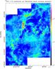 |
Fig. 1 12CO 1→0 contours of line integrated (v = −10 to 20 km s-1) emission with levels 63.5 to 381 K km s-1 in steps of 63.5 K km s-1 overlaid on a Herschel dust column-density map at 36′′ resolution (that corresponds to 0.41 pc at a distance of 1.4 kpc). This map was corrected for an average foreground contamination of Av = 5. Prominent features, such as W75N or the DR21 ridge, are indicated in the plot. DR17, 22, and 23 are H II regions. |
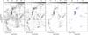 |
Fig. 2 Line integrated (v = −10 to 20 km s-1) maps (in K km s-1) of molecular emission in Cygnus X North. The lower level is zero for all maps. The blue crosses in the N2H+ map indicate submm-continuum sources (Motte et al. 2007). |
2. Observations
Molecular line data We use data from a molecular line survey of 12CO (115.3 GHz), 13CO (110.2 GHz), C18O 1→0 (109.8 GHz), CS 2→1 (98.0 GHz), and N2H+ 1→0 (93.2 GHz), which were collected with the FCRAO 14m radiotelescope between 2003 and 2006. The data were obtained using the 32 pixel Second Quabbin Optical Imaging Array (SEQUOIA) in an on-the-fly (OTF) observing mode. The beamwidth of the FCRAO at 93 GHz is ~48′′ and at 110 GHz ~45′′, while the main beam efficiency at that time was 0.48. For the present paper, we use maps on a 20′′ grid. The data have a mean 1 σrms rms noise level of ~0.4 K per 0.06 km s-1 channel on a Tmb temperature scale that we use in this paper. In the C18O map, the noise level and a slightly stripy appearance, resulting from the on-the-fly mapping mode, becomes apparent. However, this does not affect the PDFs because they are assembled from pixels above the 3σrms level. For further details, see Schneider et al. (2010, 2011).
Column-density maps from Herschel For this study, we employ a column-density map at 36′′ angular resolution (regridded to 20′′ to match the fully-sampled FCRAO maps) that were obtained as part of the HOBYS (Herschel imaging survey of OB Young Stellar objects) key program (Motte et al. 2010). This map was obtained by an SED (Spectral Energy Distribution) fit to the PACS (Poglitsch et al. 2010) 160 μm, and the SPIRE (Griffin et al. 2010) 250, 350, and 500 μm wavelengths observations. More details can be found in Appendix A and a full map of the column density of the Cygnus X North region is shown in Schneider et al. (in prep.) and Bontemps et al. (in prep.). A smaller cutout of the DR21 ridge at 25′′ resolution is presented in Hennemann et al. (2012).
3. The structure of the Cygnus X North region
Cygnus X is one of the richest star-formation regions in the Galaxy, containing the prominent OB-association Cyg OB2, with ~50 O-stars (see Reipurth & Schneider 2008 for a review). From large-scale 13CO 2→1 (Schneider et al. 2006) and 13CO 1→0 (Schneider et al. 2007) surveys, we derive a mass of a few 106M⊙ for the whole molecular cloud complex that is divided into the Cygnus X North and South regions. These studies show that the majority of the molecular clouds in the complex are located at a common distance of about 1.4–1.7 kpc. A distance of 1.4 kpc, which is derived from maser parallax (Rygl et al. 2012), is now commonly accepted. The clouds in the Cygnus X North region are actively forming stars and contain more than 100 massive pre- and protostellar dense cores (Motte et al. 2007; Bontemps 2010; Csengeri et al. 2011; Hennemann et al. 2012).
Figure 1 shows the dust column-density map of Cygnus X North with contours of 12CO 1→0 overlaid onto it. The 12CO emission is integrated over the velocity range −10 to 20 km s-1, which confines all star-forming molecular clouds that are directly associated with the Cyg OB2 cluster. Outside this velocity range, there are no other clouds along the line of sight, although in other regions of Cygnus X, clouds from the Perseus arm appear at velocities around −40 km s-1. As demonstrated in Schneider et al. (2006, see their Fig. 3), there are mainly two velocity coherent cloud complexes in Cygnus X North: the DR21 ridge-DR22-DR23 clouds at v = −10 to 1 km s-1 and the W75N-DR17 clouds at v = 7 to 20 km s-1. However, 12CO and dust also trace more diffuse emission, mainly arising from the “Great Cygnus Rift”, a nearby (0.6−1 kpc) region of obscuration, which is identified in optical images, and which is not associated with Cyg OB2. As shown in Schneider et al. (2007), the extinction due to the Rift is of the order of Av~ 5−10 and mainly arises between v=6 to 20 km s-1. Other authors determine values between Av = 2–5 (Sale et al. 2009), Av = 2.5−7 (Drew et al. 2008), Av = 5.5–7.5 (Wright et al. 2010), and Av = 2.6−5.6 (Guarcello et al. 2012). An extinction around five is also the lowest emission level in the Herschel dust map that is analysed in this paper. The Rift emission is barely detected in 13CO and not in C18O, CS, and N2H+. This means that we expect only the low column-density range of the 12CO PDF to be affected. The higher column-density power-law tail is, in any case, not affected.
Figure 2 shows the same cutout of Cygnus X North as Fig. 1 in four different line tracers. The optical depth of the lines decreases from left to right and the critical density increases. While the CO 1→0 lines have a low critical density ncr of ~103 cm-3, the CS 2→1 and the N2H+ 1→0 lines have ncr of 1.3 × 105 cm-3 and 6.1 × 104 cm-3, respectively, for a temperature of 10 K and thermal excitation (see. e.g. Flower 1999; Daniel et al. 2005; Shirley et al. 2015). In addition, CO depletes in cold and dense gas while CS, and in particular N2H+, remain stable in this gas phase. Accordingly, the maps show selectively different density regimes of the gas. While 13CO 1→0 is still sensitive to lower-density gas and resembles the 12CO map, N2H+ is confined to the densest clumps. Basically all clumps visible in the N2H+ map contain cold, dense cores (starless and protostellar, indicated by crosses in Fig. 2) observed in mm-dust continuum with the MAMBO bolometer (Motte et al. 2007). From the submm-dust observations, a typical size of 0.1 pc (0.7 pc) and density of 105 cm-3 (104 cm-3) for the cores (clumps) was derived. This value is confirmed by a decomposition of our N2H+ map using the GAUSSCLUMPS algorithm (Stutzki & Güsten 1990) in the velocity range −10 to 20 km s-1, which shows an average clump size of ~0.6 pc. We only consider clumps larger than 1.5 times the beamsize (45′′).
4. Probability distribution functions from dust and molecules
4.1. The dust PDF
As discussed in the previous section, the dust map may suffer from foreground contamination that mainly arises from the Cygnus Rift. Contamination always modifies the measured cloud PDF. Relative to the underlying PDF, the measured PDF becomes narrower, the peak shifts towards higher Av, and the slope of the power-law tail steepens (Schneider et al. 2015a). Following the method outlined in Schneider et al. (2015a), we can correct for foreground contamination by removing the constant Av = 5 value for the Cygnus Rift from the original column-density map.
For a more realistic approach, we have to take into acount, however, that the foreground contamination will typically also show a distribution of column densities, usually also following a log-normal distribution. In a systematic study, Ossenkopf et al. (in prep.) show that the correction by a constant foreground subtraction still works quite well if the most probable contaminating column density is used as the offset. This is illustrated in Fig. 4. Following the description in Schneider et al. (2015a), we contaminate a model cloud with the parameters of the Cygnus PDF with a foreground cloud that is generated from a fractional Brownian motion (fBm) map. This has a power spectral index of 2.8, which matches the typically-observed spatial scaling behaviour, and has a lognormal column-density PDF with a width ση = 0.45 and a contamination Av = 5.0. This cloud is thus a more realistic representation of a foreground or background contaminating cloud. Figure 4 shows that the contamination produces a distortion in the PDF but the simple correction obtained by subtracting a constant Av = 5.0 value fully recovers the PDF tail and recovers the PDF peak position approximately.
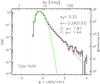 |
Fig. 3 PDF derived from the foreground-corrected Herschel column-density map. The left y-axis gives the normalized probability density p(η), the right y-axis the number of pixels per log bin. The upper x-axis is the visual extinction and the lower x-axis the natural logarithm of the normalized column density. The green curve indicates the best lognormal fit to the low column-density distribution, the red line displays a linear regression power-law fit to the high column-density tail. The dispersion of the fitted PDF (ση), the slope s and its error, and the exponent α of an equivalent spherical density distribution (C) and a cylindrical density profile, such as for filaments (F), are indicated. |
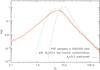 |
Fig. 4 Original PDF of a model cloud (see text) with a lognormal core and a power-law tail is shown with a green dashed line. This cloud is “contaminated” with a model cloud that has a lognormal core. The resulting PDF is shown as a blue dashed line. The red line then displays the “corrected” PDF if a constant value of Av = 5 is removed. |
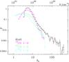 |
Fig. 5 Probability distribution functions of H2, obtained from dust and 12CO, 13CO, and C18O 1→0. All PDFs were constructed using pixels above the 3σ noise level. |
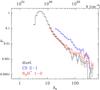 |
Fig. 6 Like Fig. 4 but showing the CS 2→1 and N2H+ 1→0 PDFs (converted into H2 column density) in addition to the dust PDF. |
Even for such a relatively strong contamination, we can thus recover the main PDF properties by subtracting a constant offset for the contamination. Figure 3 shows the N-PDF obtained from Herschel dust continuum data, corrected for a contamination of Av = 5. This dust PDF shows the typical shape of PDFs obtained for star-forming regions: a lognormal distribution for low column densities followed by a power-law distribution between Av~ 10–15 and a few hundred Av. Above Av~100, some excess in the PDF is observed that could constitute a second power law, when compared to a simple power law. Such an excess/flatter power-law tail was recently found in some massive GMCs (Schneider et al. 2015c) and was interpreted as a possible result of internal stellar feedback. The same argument may hold here because only pixels in the DR21 ridge, W75N, and some small, isolated clumps – all associated with young stellar objects (YSOs) – contribute to this high column-density part of the PDF (see Fig. 1).
4.2. The PDFs from CO
The PDFs of H2 column densities Nmol(H2), which were obtained from molecular lines, are shown in Figs. 5 and 6, together with the same dust PDF from Fig. 3. Appendix B explains in detail how Nmol(H2) was derived. In summary, we assume a constant excitation temperature of 10 K, LTE conditions, and a beam/source-filling factor of unity when determining all column densities. We note, however, that PDFs are always resolution-limited. The PDFs were constructed from pixels above the 3σ noise level and are normalized to the number of pixels from the dust map (#pixdust), i.e. we scaled the molecular line PDFs by the factor #pixmol/#pixdust. In Appendix C, we show the individual PDFs without this scaling. Above the noise level of Av~ 1–2, the Nmol(H2)-PDFs of 12CO, 13CO, and C18O can be fitted by a broad lognormal distribution with a peak at Av~ 3–5, and by a power-law tail above Av = 15 for C18O. Also, the 13CO PDF shows some excess above Av~ 15 (see Appendix C for a more detailed display).
Considering all uncertainties in the determination of H2 column density from dust and CO, the lognormal part in the CO-PDFs corresponds quite well to the lognormal part of the dust PDF, which indicates that the low-density molecular gas is probably well mixed with dust. The 12CO PDF is a special case because it is contaminated by line-of-sight confusion from the Cygnus Rift at a distance of 600 pc, and thus shifts towards lower Av to some degree. For Av larger than ~15 (we note that the column densities are correct only within a factor ~2), however the 12CO PDFs depart from the lognormal shape and the distribution becomes “bumpy” and falls off. This is the regime where the line no longer traces the dense gas because it becomes optically thick. In comparison to hydrodynamic simulations with radiative transfer (Shetty et al. 2011), our observed 12CO PDF covers a lower column-density range. Their “Milky Way cloud” (case (a) in Fig. 2) 12CO PDF has the same width but peaks around Av = 10−15. More recent results of Szücs et al. (in prep.), however, show 12CO PDFs that cover a very similar column-density range to the one we observed.
The 13CO and C18O PDFs extend to higher Av (up to ~40). The 13CO line is optically thin (τ ~ 0.1−0.3, see Fig. B.3) in most of the clouds and becomes marginally more optically thick (τ ~ 1) only in the DR21 ridge. The C18O line is optically thin everywhere with maximum values of τ ~ 0.4 in the DR21 ridge. Optical depth effects, and not depletion, are the main reason for the different PDF shapes of 12CO, 13CO, and C18O for higher column densities. The power-law behaviour for Av> 15 that we find for C18O indicates that the whole column of gas is traced up to Av~ 40. Because 13CO becomes marginally optically thin, we do not observe a clear power-law tail but only some excess because the highest column densities are no longer traced. 12CO becomes even more easily optically thick so that the high column-density pixels are not traced at all and the PDF appears lognormal. Depletion of all CO isotopologues probably sets in for Av larger than around 40 where all PDFs fall off. The removal of CO from the gas phase typically happens at densities above 104 cm-3 at temperatures ~15 K (e.g. Blake et al. 1995). Our value of Av~ 40 (N = 3.8 × 1022 cm-2) thus corresponds to a typical clump size d of ~1.25 pc (d = N/ (104 cm-3)) in which CO depletes. These clumps are the ones that are well traced by N2H+ emission and the temperature map (Fig. 8) that we discuss in the next section.
At the low Av end, approximately in the range Av = 1–2, we observe some excess compared to a purely lognormal PDF distribution for 13CO and C18O (Fig. C.1). The chemistry in this column-density regime is governed by (F)UV radiation via photodissociation (Av< 5) and fractionation (Av< 3) processes (e.g. van Dishoeck & Black 1988). The excess indicates that self-shielding of 13CO and C18O against UV-radiation is rather effective. Otherwise, the abundances would be lower and the PDF would drop more significantly. On the other hand, in warmer regions (internally or externally heated) in the medium Av range, CO desorption leads to a higher abundance of CO. These spatial abundance variations, which were observed for 13CO in Perseus (Pineda et al. 2008) and Orion (Ripple et al. 2013), have an obvious influence on the N-PDF. However, they are difficult to assess (see next section).
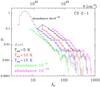 |
Fig. 7 N-Probability distribution functions obtained from CS using (i) different excitation temperatures (5, 10, 15 K) and an abundance of 4 × 10⁻¹⁰; and (ii) at a temperature of 10 K but abundance values of 10-10 and 10-9. The dust PDF is shown for comparison. |
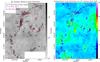 |
Fig. 8 Left: foreground-corrected dust column-density map (as shown in Fig. 1) in greyscale. The black contour indicates the Av = 15 level. The red contours show the same Av = 15 level from the H2 column-density map derived from N2H+, using an excitation temperature of 10 K and an abundance of 2 × 10⁻⁹. Right: dust temperature map of Cygnus X North from Herschel with the same red Av = 15 contour from N2H+. |
4.3. The PDFs from CS and N2H+
The Nmol(H2)-PDFs of CS and N2H+ mostly cover the high column-density range and can be best fitted by a pure power law (see Appendix C). However, all absolute values need to be taken with caution because they strongly depend on the abundance values that were used for converting column densities into H2 and on the excitation temperature.
For N2H+, we adopt [N2H+]/[H2] = 5 × 10⁻¹⁰, a value determined for massive3 cloud cores (Pigorov et al. 2003), and applied it to one of the Cygnus X North cores (N63, Motte et al. 2007) in the following way (Fechtenbaum et al., in prep.): Level population diagrams that use lines of the optically thin isotopologues 15N2H+ and N15NH+ were plotted to estimate their column density. An isotopic ratio 14N/15N of 448 (Wilson & Rood 1994) was used to derive the column density of N2H+. The mass of 44 M⊙ in a 30′′ beam (Duarte-Cabral et al. 2013) of the source enabled us to calculate the column density of H2 and thus the abundance of N2H+. The resulting PDF covers a column-density regime of Av~ 15 to 400, which corresponds very well to the one derived from dust (see Fig. 6).
For CS, there is a large scatter in observed values for high-mass star-forming regions with [CS]/[H2] = 10-9 to a few times 10-10 (Gianetti et al. 2012; Li et al. 2015; Neufeld et al. 2015). Low-mass cores have typical values of a few times 10-9 (e.g. Tafalla et al. 2006). Here, we use a value of 4 × 10⁻¹⁰ (Fechtenbaum et al., in prep.) that was obtained using the optically thin isotopologue C33S and applying the same method as outlined above. The PDF obtained with this abundance value covers the Av range ~20 to 350 and thus has a similar column density range as the PDF determined from dust, but shifted vertically to the latter.
To investigate in more detail the effects of different excitation temperatures and abundances, in Fig. 7 we plot a whole set of PDFs for CS. We first vary the excitation temperature, using 5 and 15 K as two extreme cases, and 10 K (average value determined from all molecular lines and dust). The column density variation is significant, increases its value by more than a factor two between Tex = 15 K and 5 K. Different abundance values obviously have a significant impact on the PDF as well. A lower (but unlikely) [CS]/[H2] ratio of 10-10 shifts the PDF to higher column densities with unrealistic values of a few hundred Av. A higher abundance shifts the PDF towards lower column densities, and a value of 10-9 leads to a PDF that corresponds to the one obtained from dust. In this way, it is possible to “calibrate” the [CS]/[H2] abundance using the dust PDF. However, this method should be treated with caution because the molecular line PDF also depends on the excitation temperature, and the dust PDF has its own uncertainties (variable temperature along the line of sight, unknown dust opacity etc.).
4.4. The high column density range in the maps
The PDFs obtained from dust emission and N2H+ (and CS) both show a power-law tail starting around Av~ 15. Figure 8 (left panel) illustrates the high spatial correspondence between the pixels in the dust and N2H+ maps that cover the same column-density range. The black and red contours indicate the Av = 15 level for the H2 column density derived from dust and N2H+, respectively. On average, both contours cover the same areas, implying that the dust is well mixed with the dense and cold gas that is traced by N2H+. The geometry of the emitting regions is a mixture between spherical and filamentary. Even at very high column densities (indicated by the arbitrary chosen Av = 100 blue contour from N2H+), not only spherical clumps are outlined but also the elongated DR21 ridge. An overlay between the dust temperature obtained with Herschel and the same Av = 15 contour from N2H+ (Fig. 8, right panel) shows that it is indeed mostly cold gas traced by N2H+ and dust. The clumps that are indicated by the red contour typically have a temperature of 10−15 K, except those with internal sources (the DR21 region in the DR21 ridge and DR23 at the southern border of the map). In these cases, the column density is underestimated so that the true power-law tails of both, the dust, and N2H+ PDF, which is shown in Fig. 6, are slightly flatter.
Results from the power-law fit to the PDFs.
5. Discussion and conclusions
In the following section, we base our discussion on the column density maps and PDFs of CS and N2H+ derived using an excitation temperature of 10 K and abundance values of [CS]/[H2] = 10-9 (to be consistent with the dust PDF) and [N2H+]/[H2] = 5 × 10⁻¹⁰, respectively.
5.1. Thermal and subthermal excitation regimes
For a homogeneous medium with beam-filling of unity, the H2 column-density threshold N for thermally excited N2H+ and CS calculates from the clump size (d) and critical densities with N = d × ncr. For d we adopt 0.7 pc, taken from dust submm observations (Motte et al. 2007). This value is close to the average clump size of 0.6 pc we derive from our N2H+ clump decomposition4. We thus obtain Av = 285 and 130 for CS and N2H+, respectively, assuming critical densities of 1.3 × 105 cm-3 (6.1 × 104 cm-3) for CS (N2H+). Above these values, the emission lines should be thermalized. However, the clumpiness of the gas leads to a lower threshold of thermalization. With an average density ⟨ n ⟩ = 104 cm-3 of the clumps,which was determined from submm continuum observations (Motte et al. 2007), we obtain a beam filling (⟨ n ⟩ /ncr) of ~10% for CS and ~15% for N2H+. Both lines are thus already thermalized at lower Av. For N2H+ we independently derive its thermal excitation by the hyperfine-structure line ratios. The line is mostly thermally excited because we obtain excitation temperatures above 5 K for the emitting gas (Appendix C), which is above the typical value for subthermal excitation.
CS has a higher critical density but depletes at densities above ~105 cm-3, which is consistent with our PDF that is cut off at Av~ 100 (for the abundance [CS]/[H2] = 10-9). On the other hand, its chemistry is less density dependent. Hence, we expect that CS is not thermalized at the lowest end of the distribution.
5.2. Slopes of the N-PDFs
Independent of the exact column-density regime that is covered by the PDFs from dust and CS/N2H+, they all show power-law tails with slopes s between –1.4 and –2.3 (see Table 1). The slope s of the power law can be converted into the exponent α of an equivalent density distribution ρ ∝ r− α (Appendix D). For spherical geometry, representing a single core or a core ensemble (Girichidis et al. 2014), we use αc = 1−2/s (Federrath & Klessen 2013). For singular polytropic cylinders, which portray filaments, we use αf = 1−1/s (see Toci & Galli (2015) for regular polytropic cylinder models and Fischera (2014) and Myers (2015) for the corresponding N-PDFs). The values we obtain for α (αc or αf) vary between 1.4 and 2.4. In the simplified picture of the free-fall of a collapsing sphere, α = 2 for early stages and α = 1.5 after a singularity formed at the centre of the sphere (Shu 1977; Larson 1969; Penston 1969; Whitworth & Summers 1985). Our observed values from the dust (αc = 1.9) and C18O (αc = 1.8) PDF slopes are consistent with the spherical free-fall scenario, but CS and N2H+ have higher values with αc = 2.3 and αc = 2.4, respectively. All high-density clumps traced in CS and N2H+ emission are associated with pre- and protostellar sources (Motte et al. 2007), which indicates that gravitational collapse in the star-forming phase has started. The high column densities seen in dust, CS, and N2H+ are thus not a consequence of a long column of diffuse emission, but correspond to spatially concentrated high volume densities.
On the other hand, the purely spherical free-fall picture seems unlikely to apply to most of the gas which defines the N-PDF power laws, because most of the gas we observe in Cygnus X is filamentary. This is clearly illustrated in the maps shown in Figs. 1, 2, and 7, which display the filamentary network in the CO lines and, with only a small fraction of gas in cores, that could be considered roughly spherical (see CS and N2H+ maps in Figs. 2 and 7 and submm continuum observations in Motte et al. 2007)5. Filaments can be in global free-fall collapse, as suggested by molecular line observations (e.g. Peretto et al. 2013; Schneider et al. 2010, 2015b) but the gas we see in filaments (and cores) can account for power-law N-PDFs if it has the right power-law radial-density structure, even in hydrostatic balance with no net inward motion. The observed N-PDF slopes (s = −1.4 to −2.6, leading to αf between 1.4 and 1.7) are consistent with self-gravitating but non-collapsing filament models (Myers 2015; Toci & Galli 2015). In this case, filamentary gas that has a sufficient mass per length ratio is centrally concentrated and self-gravitating, but does not need to be globally collapsing. However, to confine the filaments/clumps, an external pressure pext ∝ ⟨ n ⟩ Tkin of the order of pext ~ 104−5 cm-3 × 10 K is required (where ⟨ n ⟩ is the average density in the filaments/clumps and Tkin the gas temperature). However, this pressure cannot be isotropic, provided by the lower density envelope that is well traced in 12CO at a density of ~103 cm-3 and a temperature of ~10−40 K. Moreover, it could be ram pressure of new gas that is accreting onto filaments and clumps, a process that is now frequently observed (e.g. Schneider et al. 2010; Kirk et al. 2013; Palmeirim et al. 2013).
The flatter power-law slopes of the CS and N2H+ PDF in comparison to the dust could reflect an abundance change because N2H+ is produced when CO is depleted at very high column densities (Bergin et al. 2001; Tafalla et al. 2002, 2002). In addition, because CS is not thermalized at the lowest column densities, this could lead to a somewhat flatter tail with respect to the dust.
In summary, a power-law distribution in the density structure is required to have a power-law tail in the PDF and this can be achieved by either a hydrostatic configuration, where the power law arises from a balance of gravitational forces and pressure gradients, or directly in a dynamically collapsing system. Probably both play a role, with filaments possibly balanced or at least contraction-slowed by (magnetic) pressure gradients on the one hand and very dense collapsing cores on the other.
6. Summary
We derived probability distribution functions (N-PDFs) of H2 column density for the Cygnus X North region from dust, 12CO, 13CO, C18O 1→0, CS 2→1, and N2H+ 1→0. The determination of the H2 column density from the molecular lines is based on standard procedures and abundances, assuming a common excitation temperature of 10 K and LTE. Our findings are:
-
The PDFs of dust and CO isotopologues can be described by alognormal distribution for the low column-density rangebetween Av~ 1 to ~15, with a common peak around Av~ 5. Though line-of-sight contamination and variations in abundance and excitation temperatures introduce large uncertainties in the CO-PDFs, the overall correspondence between these observational PDFs and the ones from recent simulations (Szücs et al. 2015) is good.
-
Optical depth effects are the main reason for the different PDF shapes of 12CO, 13CO, and C18O for higher column densities. The PDF from 12CO is cut above Av~ 30 because the line becomes optically thick. The marginally optically thin 13CO line shows excess in its PDF for Av = 15−40, while the PDF for the optically thin C18O line displays a power-law tail in the same Av = 15−40 range.
-
Neither selective photodissociation nor fractionation seem to play a significant role for the CO abundances for low column densities.
-
Depletion of all CO isotopologues probably sets in for Av greater than around 40 where all PDFs fall off.
-
The PDFs of CS and N2H+ only consist of a power-law tail that covers a high column density range (Av~ 15 to a few 100 Av). Using CS as an example, we discuss the potential influence of abundance and excitation temperature variations, and show that these could shift the entire PDF by more than one magnitude in column density. To better constrain this uncertainty, we “calibrate” the molecular line PDF using the dust-emission map (i.e. shifting the distribution at a given excitation temperature so that it corresponds to the dust PDF). For CS, we obtain an abundance of [CS]/[H2] = 10-9 in this way.
-
We find that the N2H+ and CS lines are mainly thermally excited. N2H+ is well mixed with the dust and traces spatially the same dense gas clumps of a typical size of ~0.6−0.7 pc that were shown to contain pre- and protostellar sources (Motte et al. 2007).
-
The slopes of the high column-density power-law tail end of the N-PDFs from dust, CS, and N2H+ are s = −2.3, −1.6, and −1.4, respectively. These values are consistent with a gas distribution that is dominated by gravity, i.e. free-falling gas in cores and filaments, although a hydrostatic configuration with ram pressure by gas accretion can also take place. The power law then arises from a balance of gravitational forces and pressure gradients.
Summarising the observational results, we find that the N-PDFs obtained from molecular lines are not well confined because they depend strongly on excitation temperature and abundance, and various combinations of these can lead to the same PDF. “Calibrating” a molecular line PDF with dust is an appealing approach but it should be kept in mind that dust PDFs also suffer from uncertainties. For example, the specific dust opacity is not constant (a value of β = 2 was chosen for this paper) and line-of-sight contamination can lead to an overestimation of the column density. However, this study nevertheless shows that the dust provides the highest dynamic range in tracing the low to high column-density regime, compared to the molecular line tracers (see also Goodman et al. 2009; and Burkhart et al. 2013).
The column density N can be expressed as visual extinction Av with N(H2) = Av 0.94 × 1021 cm-2 mag-1 (Bohlin et al. 1978).
In Aquila (Könyves et al. 2015) the power-law tail contains more than ~50% of the mass in filaments but only ~15% in cores.
Acknowledgments
N.S. and S.B. acknowledge support by the ANR-11-BS56-010 project STARFICH. N.S., V.O., and T.C. acknowledge support from the Deutsche Forschungsgemeinschaft, DFG, through project number 0s 177/2-1 and 177/2-2, and central funds of the DFG-priority program 1573 (ISM-SPP). C.F. acknowledges funding provided by the Australian Research Councils Discovery Projects (grants DP130102078 and DP150104329). R.S.K. acknowledges subsidies from the DFG priority program 1573 (Physics of the Interstellar Medium) and the collaborative research project SFB 881 (The Milky Way System, subprojects B1, B2, and B5).
References
- Alves de Oliveira, C., Schneider, N., Merin, B., et al. 2014, A&A, 568, A98 [NASA ADS] [CrossRef] [EDP Sciences] [Google Scholar]
- Bergin, E. A., Ciardi, D. R., & Lada, C. 2001, ApJ, 557, 209 [NASA ADS] [CrossRef] [Google Scholar]
- Blake, G. A., Sandell, G., van Dishoeck, E. F., et al. 1995, ApJ, 441, 689 [Google Scholar]
- Bohlin, R. C., Savage, B. D., & Drake, J. F. 1978, ApJ, 224, 132 [NASA ADS] [CrossRef] [Google Scholar]
- Bontemps, S., Motte, F., Csengeri, T., et al. 2010, A&A, 524, A18 [NASA ADS] [CrossRef] [EDP Sciences] [Google Scholar]
- Bolatto, A. D., Wolfire, M., & Leroy, A. K. 2013, ARA&A, 51, 207 [Google Scholar]
- Burkhart, B., Ossenkopf, V., Lazarian, A., & Stutzki, J. 2013, ApJ, 771, 122 [NASA ADS] [CrossRef] [Google Scholar]
- Carlhoff, P., Schilke, P., Nguyen-Luong, Q., et al. 2013, A&A, 560, A24 [NASA ADS] [CrossRef] [EDP Sciences] [Google Scholar]
- Caselli, P., Benson, P. J., Myers, P. C., & Tafalla, M. 2002, ApJ, 572, 238 [NASA ADS] [CrossRef] [Google Scholar]
- Csengeri, T., Bontemps, S., Schneider, N., et al. 2011, A&A, 527, A135 [NASA ADS] [CrossRef] [EDP Sciences] [Google Scholar]
- Daniel, F., Dubernet, M.-L., Meuwly, M., et al. 2005, MNRAS, 363, 1083 [NASA ADS] [CrossRef] [Google Scholar]
- Drew, J. E., Greimel, R., Irwin, M. J., & Sale, S. E. 2008, MNRAS, 386, 1761 [NASA ADS] [CrossRef] [Google Scholar]
- Duarte-Cabral, A., Bontemps, S., Motte, F., et al. 2013, A&A, 558, A125 [NASA ADS] [CrossRef] [EDP Sciences] [Google Scholar]
- Federrath, C., & Klessen, R. S. 2012, ApJ, 761, 156 [NASA ADS] [CrossRef] [Google Scholar]
- Federrath, C., & Klessen, R. S. 2013, ApJ, 763, 51 [NASA ADS] [CrossRef] [Google Scholar]
- Federrath, C., Klessen, R. S., & Schmidt, W. 2008, ApJ, 688, L79 [NASA ADS] [CrossRef] [Google Scholar]
- Federrath, C., Roman-Duval, J., Klessen, R. J., et al. 2010, A&A, 512, A81 [NASA ADS] [CrossRef] [EDP Sciences] [Google Scholar]
- Fischera, J. 2014, A&A, 571, A95 [NASA ADS] [CrossRef] [EDP Sciences] [Google Scholar]
- Flower, D. R. 1999, MNRAS, 305, 651 [NASA ADS] [CrossRef] [Google Scholar]
- Fontani, F., Giannetti, A., Beltran, M. T., et al. 2012, MNRAS, 423, 2342 [NASA ADS] [CrossRef] [Google Scholar]
- Frerking, M. A., Langer, W. D., & Wilson, R. W. 1982, ApJ, 262, 590 [NASA ADS] [CrossRef] [Google Scholar]
- Froebrich, D., & Rowles, J. 2010, MNRAS, 406, 1350 [NASA ADS] [Google Scholar]
- Gianetti, A., Brand, J., Massi, F., et al. 2012, A&A, 538, A41 [NASA ADS] [CrossRef] [EDP Sciences] [Google Scholar]
- Girichidis, P., Konstandin, L., Whitworth, A. P., Klessen, R., et al. 2014, ApJ, 781, 91 [NASA ADS] [CrossRef] [Google Scholar]
- Goldsmith, P. F., Heyer, M., Narayanan, G., et al. 2008, ApJ, 680, 428 [NASA ADS] [CrossRef] [Google Scholar]
- Goodman, A. A., Pineda, J. E., & Schnee, S. L. 2009, ApJ, 692, 91 [NASA ADS] [CrossRef] [Google Scholar]
- Griffin, M., Abergel, A., Abreau, S., et al. 2010, A&A, 518, L3 [Google Scholar]
- Guarcello, M. G., Wright, N. J., Drake, J. J., et al. 2012, ApJS, 202, 19 [NASA ADS] [CrossRef] [Google Scholar]
- Hennebelle, P., & Chabrier, G. 2008, ApJ, 684, 395 [NASA ADS] [CrossRef] [Google Scholar]
- Hennemann, M., Motte, F., Schneider, N., et al. 2012, A&A, 543, L3 [NASA ADS] [CrossRef] [EDP Sciences] [Google Scholar]
- Hill, T., Motte, F., Didelon, P. et al. 2011, A&A, 533, A94 [NASA ADS] [CrossRef] [EDP Sciences] [Google Scholar]
- Hopkins, P. F. 2013, MNRAS, 423, 2037 [Google Scholar]
- Kainulainen, J., Beuther, H., Henning, T., & Plume, R. 2009, A&A, 508, L35 [NASA ADS] [CrossRef] [EDP Sciences] [Google Scholar]
- Kirk, H., Myers, P. C., Bourke, T. L., et al. 2013, ApJ, 766, 115 [NASA ADS] [CrossRef] [Google Scholar]
- Klessen, R. S. 2000, ApJ, 535, 869 [NASA ADS] [CrossRef] [Google Scholar]
- Könyves, V., André, P., Men’shchikov, A., et al. 2015, A&A, 584, A91 [NASA ADS] [CrossRef] [EDP Sciences] [Google Scholar]
- Krumholz, M., & McKee, C. F. 2005, ApJ, 630, 250 [NASA ADS] [CrossRef] [Google Scholar]
- Langer, W. D., & Penzias, A. A. 1990, ApJ, 357, 477 [NASA ADS] [CrossRef] [Google Scholar]
- Larson, R. B. 1969, MNRAS, 145, 271 [NASA ADS] [CrossRef] [Google Scholar]
- Li, J., Wang, J., Zhu, Q., et al. 2015, ApJ, 802, 40 [NASA ADS] [CrossRef] [Google Scholar]
- Lo, N., Cunningham, M. R., Jones, P. A., et al. 2009, MNRAS, 395, 1021 [NASA ADS] [CrossRef] [Google Scholar]
- Lombardi, M., Lada, C., & Alves, J. 2008, A&A, 489, 143 [NASA ADS] [CrossRef] [EDP Sciences] [Google Scholar]
- Mangum, J. G., & Shirley, Y. L. 2015, PASP, 127, 266 [NASA ADS] [CrossRef] [Google Scholar]
- Motte, F., Bontemps, S., Schilke, P., et al. 2007, A&A, 476, 1243 [NASA ADS] [CrossRef] [EDP Sciences] [Google Scholar]
- Motte, F., Zavagno, A., Bontemps, S., et al. 2010, A&A, 518, L77 [NASA ADS] [CrossRef] [EDP Sciences] [Google Scholar]
- Myers, P. C. 2015, ApJ, 806, 226 [NASA ADS] [CrossRef] [Google Scholar]
- Neufeld, D. A., Godard, B., Gerin, M., et al. 2015, A&A, 577, A49 [NASA ADS] [CrossRef] [EDP Sciences] [Google Scholar]
- Padoan, P., & Nordlund, A. 2011, ApJ, 741, 22 [Google Scholar]
- Palmeirirm, P., André, P., Kirk, J., et al. 2013, A&A, 550, A38 [NASA ADS] [CrossRef] [EDP Sciences] [Google Scholar]
- Penston, M. V. 1969, MNRAS, 144, 425 [NASA ADS] [CrossRef] [Google Scholar]
- Peretto, N., Fuller, G. A., Duarte-Cabral, A., et al. 2013, A&A, 555, A112 [NASA ADS] [CrossRef] [EDP Sciences] [Google Scholar]
- Pineda, J. E., Caselli, P., & Goodman, A. 2008, ApJ, 679, 481 [NASA ADS] [CrossRef] [Google Scholar]
- Pineda, J. L., Goldsmith, P. F., Chapman, N., et al. 2010, ApJ, 721, 686 [NASA ADS] [CrossRef] [Google Scholar]
- Pigorov, L., Zinchenko, I., Caselli, P., et al. 2003, A&A, 405, 639 [NASA ADS] [CrossRef] [EDP Sciences] [Google Scholar]
- Poglitsch, A., Waelkens, C., Geis, N., et al. 2010, A&A, 518, L2 [NASA ADS] [CrossRef] [EDP Sciences] [Google Scholar]
- Reipurth, B., Schneider, N. 2008, Handbook of star forming regions, Vol. I, ASP Publ., ed. B. Reipurth, 36 [Google Scholar]
- Ripple, F., Heyer, M. H., Gutermuth, R., et al. 2013, MNRAS, 431, 1296 [NASA ADS] [CrossRef] [Google Scholar]
- Russeil, D., Schneider, N., Anderson, L., et al. 2013, A&A, 554, A42 [NASA ADS] [CrossRef] [EDP Sciences] [Google Scholar]
- Rygl, K. L. J., Brunthaler, A., Sanna, A., et al. 2012, A&A, 539, A79 [NASA ADS] [CrossRef] [EDP Sciences] [Google Scholar]
- Sale, S. E., Drew, J. E., Unruh, Y. C., et al. 2009, MNRAS, 392, 497 [NASA ADS] [CrossRef] [Google Scholar]
- Schneider, N., Bontemps, S., Simon, R., et al. 2006, A&A, 458, 855 [NASA ADS] [CrossRef] [EDP Sciences] [Google Scholar]
- Schneider, N., Simon, R., Bontemps, S, et al. 2007, A&A, 474, 873 [NASA ADS] [CrossRef] [EDP Sciences] [Google Scholar]
- Schneider, N., Csengeri, T., Bontemps, S., et al. 2010, A&A, 520, A49 [NASA ADS] [CrossRef] [EDP Sciences] [Google Scholar]
- Schneider, N., Bontemps, S., Simon, R., et al. 2011, A&A, 529, L1 [NASA ADS] [CrossRef] [EDP Sciences] [Google Scholar]
- Schneider, N., Csengeri, T., Hennemann, M., et al. 2012, A&A, 540, L11 [NASA ADS] [CrossRef] [EDP Sciences] [Google Scholar]
- Schneider, N., André, Ph., Könyves, V., Bontemps, S., et al. 2013, ApJ, 766, L17 [NASA ADS] [CrossRef] [Google Scholar]
- Schneider, N., Ossenkopf, V., Csengeri, T., et al. 2015a, A&A, 575, A79 [NASA ADS] [CrossRef] [EDP Sciences] [Google Scholar]
- Schneider, N., Csengeri, T., Klessen, R. S., et al. 2015b, A&A, 578, A29 [NASA ADS] [CrossRef] [EDP Sciences] [Google Scholar]
- Schneider, N., Bontemps, S., Girichidis, P., et al. 2015c, MNRAS, 453, L41 [CrossRef] [Google Scholar]
- Shirley, Y. L. 2015, PASP, 127, 299 [NASA ADS] [CrossRef] [Google Scholar]
- Shetty, R., Glover, S. C., Dullemond, C. P., & Klessen, R. S. 2011, MNRAS, 412, 1686 [NASA ADS] [CrossRef] [MathSciNet] [Google Scholar]
- Shu., F. 1977, ApJ, 214, 488 [NASA ADS] [CrossRef] [Google Scholar]
- Strong, J., Bloemen, J., Dame, T., et al. 1988, A&A, 207, 1 [NASA ADS] [Google Scholar]
- Stutzki, J., & Güsten, R. 1990, ApJ, 356, 513 [NASA ADS] [CrossRef] [Google Scholar]
- Stutz, A. M., & Kainulainen, J. 2015, A&A, 577, L6 [NASA ADS] [CrossRef] [EDP Sciences] [Google Scholar]
- Tafalla, M., Myers, P. C., Caselli, P., & Walmsley, C. M. 2002, ApJ, 569, 815 [NASA ADS] [CrossRef] [Google Scholar]
- Tafalla, M., Santiago-Garcia, J., Myers, P. C., et al. 2006, A&A, 455, 577 [NASA ADS] [CrossRef] [EDP Sciences] [Google Scholar]
- Toci, C., & Galli, D. 2015, MNRAS, 446, 2118 [NASA ADS] [CrossRef] [Google Scholar]
- Tremblin, P., Schneider, N., Minier, V., et al. 2014, A&A, 564, A106 [NASA ADS] [CrossRef] [EDP Sciences] [Google Scholar]
- Vázquez-Semadeni, E., & Garcia, N. 2001, ApJ, 557, 727 [NASA ADS] [CrossRef] [Google Scholar]
- Van Dishoeck, E. F., & Black, 1988, ApJ, 334, 771 [NASA ADS] [CrossRef] [Google Scholar]
- Ward, R. L., Wadsley, J., & Sills, A. 2014, MNRAS, 445, 1575 [NASA ADS] [CrossRef] [Google Scholar]
- Wilson, T. L., & Rood, R. 1994, ARA&A, 32, 191 [NASA ADS] [CrossRef] [Google Scholar]
- Whitworth, A., & Summers 1985, MNRAS, 214, 1 [NASA ADS] [CrossRef] [Google Scholar]
- Wong, T., Ladd, E. F., Brisbin, D., et al. 2008, MNRAS, 386, 1069 [NASA ADS] [CrossRef] [Google Scholar]
- Wright, N. J., Drake, J. J., Drew, J. E., & Vink, J. S. 2010, ApJ, 713, 871 [NASA ADS] [CrossRef] [Google Scholar]
Appendix A: Determination of H2 column density from dust
We assume optically thin dust emission at one dust temperature Td for each pixel in the map and fitted a greybody function of the form Iν = Bv(Td) κ Σ to the absolutely calibrated datapoints at 160 μm, 250 μm, 350 μm, and 500 μm. The specific dust opacity per unit mass (dust+gas) is approximated by the power law κν = 0.1 (ν/ 1000 GHz)β cm2/g with β = 2, and the dust temperature and surface density distribution Σ are left as free parameters. The H2 column density Ndust is then calculated from Σ = μHmHNdust, adopting a mean molecular weight per hydrogen molecule μH = 2.8. For more details, see Hill et al. (2011). We approximate the final uncertainties in the dust column-density maps to be around ~30−50%, mainly as a result of the uncertainty in the assumed form of the opacity law and possible temperature gradients along the line of sight.
Appendix B: Determination of H2 column density from molecular lines
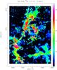 |
Fig. B.1 Map of excitation temperature of the main velocity component in Cygnus X North obtained from a Gaussian fit to the 12CO 1→0 line. |
Appendix B.1: Determination of and constraints on the excitation temperature
The temperature stucture in the Cygnus X North region is complex. Large-scale UV illumination from the central Cyg OB2 cluster heats the diffuse gas and PDR surfaces. Internal (proto)-stars and clusters such as DR21 show up as local hotspots. In parallel, the Cygnus X North clouds also contain a large reservoir of cold and dense gas, seen in submm continuum (Motte et al. 2007).
The observations of several molecular lines enable us to trace sensitively this temperature structure. If the LTE assumption is valid and the density is larger than the critical density of the transition, the kinetic temperature of the gas (Tkin) corresponds to the excitation temperature Tex for the molecular lines (which is assumed to be equal for all species). If gas and dust are well mixed, this temperature should also correspond to the dust temperature Tdust that was derived from Herschel. However, LTE conditions are not present and the density varies from low values in the diffuse gas phase, mainly seen in 12CO, to high values in dense clumps in the molecular clouds, traced by dust and the CS and N2H+ lines. In the following, we determine the excitation temperature in different ways, using the observational data sets.
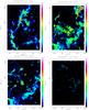 |
Fig. B.2 Maps of the Gaussian fits to the main-beam brightness temperature of 13CO 1→0 for the four main velocity ranges in Cygnus X North. The most prominent emission comes from the velocity component at −4 km s-1. |
Texfrom 12CO 1→0 From 12CO 1→0, we calculate the excitation temperature assuming that this line is optically thick so that 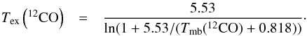 (B.1)The molecular clouds in the Cygnus region consist of several velocity components (Schneider et al. 2006). We performed a Gaussian line fit to the four main lines (see explanations for the 13CO column density). Figure B.1 shows the resulting excitation temperature for the most prominent component at velocities around −4 km s-1. It becomes obvious that the temperature varies significantly between ~5 and ~40 K.
Texfrom N2H+ 1→0 We calculate the excitation temperature from N2H+ by fitting its hyperfine structure with the known relative intensities of the seven components. The fit delivers simultaneously the opacity τ and Tex and shows no anomaly in the relative intensities. The average value of Tex is 7 K (in a range of 5 to 20 K) and the opacity is generally below one. However, we emphasise that only the product τ × Tex is constrained by the fit so that the excitation temperature is not well constrained.
Texfrom dust The right-hand panel of Fig. 6 shows the dust temperature we derive from the SED fit to the Herschel fluxes. The average value for the dust temperature across the map is 15 K, with a variation between 10 and 25 K (see also Hennemann et al. 2012). Because the dust temperature is an average along the line of sight, it is not well determined in regions with strong temperature gradients. However, for cold, dense clumps and cores that are associated with CS and N2H+ emission, we expect a much smaller variation in temperature.
In summary, considering the excitation temperatures determined from the molecular lines and the dust, we use 10 K in the following as the best compromise for the determination of column densities. However, we also discuss other methods (using Tex from 12CO) to obtain the 13CO column density, and study the influence of different Tex for the N2H+ column density.
Appendix B.2: Column densities from linear molecules
The beam-averaged total column density N of any optically thin molecule can be determined from the observed line-integrated main-beam brightness temperature Tmb with ![\appendix \setcounter{section}{2} \begin{eqnarray} {N} \, [{\rm cm}^{-2}] & = & f(T_{\rm ex}) \int {T}_{\rm mb} [K] \, {\rm d}{v}\rm [km ~s^{-1}] \nonumber \\ \end{eqnarray}](/articles/aa/full_html/2016/03/aa27144-15/aa27144-15-eq103.png) (B.2)and for linear molecules
(B.2)and for linear molecules ![\appendix \setcounter{section}{2} \begin{eqnarray} f(T_{\rm ex}) & = & \frac{3hZ}{8 \pi^3 \mu^2 J_{\rm u}} \frac{\exp(E_{\rm up}/kT_{\rm ex})}{[1-\exp(-h\nu/kT_{\rm ex})] (J(T_{\rm ex}) - J(T_{\rm BG}))} \nonumber \\ & & \label{ncol} \end{eqnarray}](/articles/aa/full_html/2016/03/aa27144-15/aa27144-15-eq104.png) (B.3)and
(B.3)and 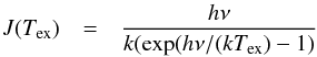 (B.4)and J(TBG) = J(2.7K), and in which h and k denote the Planck and the Boltzman constants, respectively, Eup is the energy of the upper level, ν is the frequency [GHz], μ is the dipole moment [Debye], Ju is the upper value of the rotational quantum number and
  is the velocity integrated line intensity on a main beam temperature scale.
The first two terms of the rotational partition function for a diatomic linear molecule which is accurate to 1%, compared to the full term for temperatures above 2 K (Mangum & Shirley 2015), are given by  (B.5)with the rotational constant B expressed to first order as ν = 2BJu.
To determine all H2 column densities, we apply a correction to the hydrogen mass of a factor of 1.36 to account for helium and other heavy elements.
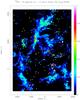 |
Fig. B.3 Map of the 13CO opacity derived for the velocity component −4 km s-1. White pixels indicate positions that were not well-fitted (e.g. FWHM too large, intensities too low) and thus attributed a blanking value. |
H2 column density from 13CO 1→0 The values for the 13CO 1→0 transition are ν = 110.201 GHz, hν/k = 5.29 K, μ = 0.112 Debye, Ju = 1, and J(2.7K) = 0.868. The temperature-dependent factor f(Tex) is 3.22, 2.00, 1.62, 1.58, and 1.70 × 10¹⁵ K-1 (km s-1)-1 cm-2 for 5, 7, 10, 15, and 20 K, respectively. As discussed above, we use a constant value of 10 K for Tex. A change in the excitation temperature between 5 and 15 K implies only a 10% variation in the column-density value. We then use an abundance [12C]/[13C] = 70, determined from Wilson & Rood (1994). This value corresponds well to the one derived for Orion A (Langer & Penzias 1990). For the [H2]/[12CO] abundance, we use a value of 1.1 × 10⁴ (Pineda et al. 2010; Fontani et al. 2012).
Because it is known that the 13CO 1→0 line is not always optically thin, an opacity correction τ13/ (1−exp(τ13)) for moderate τ can be applied for the column density (Frerking et al. 1982). To verify if this kind of correction is required, we determine the 13CO opacity by using the excitation temperature Tex that was obtained from 12CO and the observed 13CO main-beam brightness temperature Tmb(13CO) with  (B.6)Because the molecular clouds in the Cygnus region consist of several velocity features (Schneider et al. 2006), we perform a Gaussian line fit to four components for 12CO and 13CO (see B.1). As shown in Fig. B.2, the dominating emission comes from the component at −4 km s-1, which is associated with the molecular clouds of DR21, DR22, and DR23. The component at 9 km s-1 becomes important for the W75 region and southwest of the DR21 ridge. Emission at 3 and 15 km s-1 is more diffuse and on a low intensity level. We calculate the 13CO opacity for all velocity components and find that the line is optically thin everywhere, even for the −4 km s-1 component that is shown in Fig. B.3. We thus did not include an opacity correction for the determination of the 13CO column density.
The N-PDFs that were determined from the 13CO column density, using a constant excitation temperature of 10 K or a variable pixel-to-pixel temperature Tex from 12CO, do not show a significant difference.
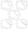 |
Fig. C.1 PDFs derived from the molecular line maps. The left y-axis gives the normalized probability p(η), the right y-axis the number of pixels per log bin. The upper x-axis is the visual extinction and the lower x-axis the logarithm of the normalized column density. For the CO lines, we fitted a lognormal to the low column-density range, indicated by a green curve. The red line shows the power-law fit to the high column-density end for C18O, CS, and N2H+. The respective slopes s (and errors) are given in the panels. For the CO lines, the peak and width of the PDF is indicated with Avpeak and σ. |
H2column density from C18O 1→0 The values for the C18O 1→0 transition are ν = 109.782 GHz, hν/k = 5.27 K, μ = 0.1098 Debye, Ju = 1, and J(2.7 K) = 0.872 K. The temperature-dependent factor f(Tex) is 3.34, 2.08, 1.69, 1.65, and 1.78 × 10¹⁵ K-1 (km s-1)-1 cm-2 for 5, 7, 10, 15, and 20 K, respectively. As discussed in Sect. B.1, we adopt a value of 10 K for Tex. To determine the H2 column density, we then use a ratio [H2]/[12CO] of 1.1 × 10⁴ (Pineda et al. 2010; Fontani et al. 2012) and an abundance [16O]/[18O] = 531, which was determined from Wilson & Rood (1994), using a distance of 1.4 kpc.
We determine the C18O opacity in the same way for the four line components as we did for 13CO (see above), using the excitation temperature Tex obtained from 12CO and the observed C18O main-beam brightness temperature Tmb(C18O) with  (B.7)Maps of the resulting C18O opacity show that the line is optically thin for all velocity components and reaches its maximum value of τ18 ~ 0.4 only in the DR21 ridge for the −4 km s-1 component.
H2 column density from 12CO 1→0 The 12CO 1→0 line is optically thick so that it should a priori not be a good tracer for the total column density. However, empirical studies (Strong et al. 1988; Bolatto et al. 2013) show that the line still can trace the total column density/mass of a molecular cloud reasonably well with a conversion factor of 2−2.3 × 10²⁰ from line integrated CO main-beam brightness temperature into H2 column density. Here, we adopt a value of 2 × 10²⁰ K-1 (km s-1)-1 cm-2.
H2 column density from CS 2→1 The values for the CS 2→1 transition are ν = 98.0 GHz, hν/k = 4.70 K, μ = 1.95 Debye, Ju = 2, and J(2.7 K) = 1.00. The factor f(Tex) is 16.1, 9.48, 7.35, 7.00, and 7.41 × 10¹² K-1 (km s-1)-1 cm-2 for 5, 7, 10, 15, and 20 K. We assume optically thin CS emission and an abundance [CS]/[H2] of 4 × 10⁻¹⁰ (Fechtenbaum et al., in prep.).
H2 column density from N2H+ 1→0 The values for the N2H+ 1→0 transition are ν = 93.17 GHz, hν/k = 4.47 K, μ = 3.40 Debye, Ju = 1, and J(2.7K) = 1.06. The factor f(Tex) is 3.62, 2.44, 2.10, 2.16, and 2.39 × 10¹² K-1 (km s-1)-1 cm-2 for 5, 7, 10, 15, and 20 K. The total beam averaged N2H+ column density is calculated using the line-integrated emission from the F = (2,1) J = (1,0) component at a frequency of 93.1737767 GHz and a HFS intensity ratio of 7/27 for that component. We assume an abundance [N2H+]/[H2] of 5 × 10⁻¹⁰.
We emphasise that all H2 column-density determinations have a large uncertainty, mainly arising from the abundance. The [CO]/[H2] abundance for the CO isotopolgues is probably better constrained because it has been well studied in the literature. However, the variation in excitation temperature along the line of sight is more significant here because the CO lines trace a larger range in densities and temperatures than the high-density tracers CS and N2H+. For the latter, the constant excitation temperature assumption is most likely more valid, but the abundances of CS and N2H+ are less well constrained, in particular for massive clumps and cores. In summary, we consider the H2 column densities from CO to be correct within a factor of two and the ones from CS and N2H+ within a factor of a few.
Appendix C: Individual molecular line PDFs
In the main body of the paper, we used a normalization for the PDF with respect to the size, i.e. pixel number of the dust map. We here show the PDFs obtained with a normalization  . As such, the PDFs are consistent with what is shown in the literature (see Schneider et al. 2015a, and references therein) and the number of pixels defining the PDF can be extracted. Figure C.1 shows the resulting PDFs.
Appendix D: Relation between PDF slope and radial density distribution for different geometries
We define the PDF pN as the surface fraction with gas of column density N and the PDF of the natural log of the column density density pη with η = ln(N/ ⟨ N ⟩), the relation between the two is pη = NpN. The definition of pN gives pN ∝ dA/ dN.
Spherical geometry In the case of spherical geometry, the density radial profile is ρ(r) ∝ r− α, hence N ∝ ρr ∝ r− α + 1 (dN ∝ r− α). Hence, with the area A ∝ r2 (dA ∝ r) 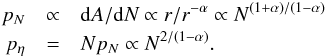 (D.1)Cylindrical geometry In the case of cylindrical geometry, the density radial profile from the axis of the cylinder is
  , hence
  . However in this case A ∝ z × rc ∝ rc, hence
 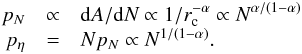 (D.2)Note that similar calculations can be found in Federrath & Klessen (2013), Fischera et al. (2014), and Myers (2015).
All Tables
All Figures
|
Fig. 1 12CO 1→0 contours of line integrated (v = −10 to 20 km s-1) emission with levels 63.5 to 381 K km s-1 in steps of 63.5 K km s-1 overlaid on a Herschel dust column-density map at 36′′ resolution (that corresponds to 0.41 pc at a distance of 1.4 kpc). This map was corrected for an average foreground contamination of Av = 5. Prominent features, such as W75N or the DR21 ridge, are indicated in the plot. DR17, 22, and 23 are H II regions. |
| In the text | |
|
Fig. 2 Line integrated (v = −10 to 20 km s-1) maps (in K km s-1) of molecular emission in Cygnus X North. The lower level is zero for all maps. The blue crosses in the N2H+ map indicate submm-continuum sources (Motte et al. 2007). |
| In the text | |
|
Fig. 3 PDF derived from the foreground-corrected Herschel column-density map. The left y-axis gives the normalized probability density p(η), the right y-axis the number of pixels per log bin. The upper x-axis is the visual extinction and the lower x-axis the natural logarithm of the normalized column density. The green curve indicates the best lognormal fit to the low column-density distribution, the red line displays a linear regression power-law fit to the high column-density tail. The dispersion of the fitted PDF (ση), the slope s and its error, and the exponent α of an equivalent spherical density distribution (C) and a cylindrical density profile, such as for filaments (F), are indicated. |
| In the text | |
|
Fig. 4 Original PDF of a model cloud (see text) with a lognormal core and a power-law tail is shown with a green dashed line. This cloud is “contaminated” with a model cloud that has a lognormal core. The resulting PDF is shown as a blue dashed line. The red line then displays the “corrected” PDF if a constant value of Av = 5 is removed. |
| In the text | |
|
Fig. 5 Probability distribution functions of H2, obtained from dust and 12CO, 13CO, and C18O 1→0. All PDFs were constructed using pixels above the 3σ noise level. |
| In the text | |
|
Fig. 6 Like Fig. 4 but showing the CS 2→1 and N2H+ 1→0 PDFs (converted into H2 column density) in addition to the dust PDF. |
| In the text | |
|
Fig. 7 N-Probability distribution functions obtained from CS using (i) different excitation temperatures (5, 10, 15 K) and an abundance of 4 × 10⁻¹⁰; and (ii) at a temperature of 10 K but abundance values of 10-10 and 10-9. The dust PDF is shown for comparison. |
| In the text | |
|
Fig. 8 Left: foreground-corrected dust column-density map (as shown in Fig. 1) in greyscale. The black contour indicates the Av = 15 level. The red contours show the same Av = 15 level from the H2 column-density map derived from N2H+, using an excitation temperature of 10 K and an abundance of 2 × 10⁻⁹. Right: dust temperature map of Cygnus X North from Herschel with the same red Av = 15 contour from N2H+. |
| In the text | |
|
Fig. B.1 Map of excitation temperature of the main velocity component in Cygnus X North obtained from a Gaussian fit to the 12CO 1→0 line. |
| In the text | |
|
Fig. B.2 Maps of the Gaussian fits to the main-beam brightness temperature of 13CO 1→0 for the four main velocity ranges in Cygnus X North. The most prominent emission comes from the velocity component at −4 km s-1. |
| In the text | |
|
Fig. B.3 Map of the 13CO opacity derived for the velocity component −4 km s-1. White pixels indicate positions that were not well-fitted (e.g. FWHM too large, intensities too low) and thus attributed a blanking value. |
| In the text | |
|
Fig. C.1 PDFs derived from the molecular line maps. The left y-axis gives the normalized probability p(η), the right y-axis the number of pixels per log bin. The upper x-axis is the visual extinction and the lower x-axis the logarithm of the normalized column density. For the CO lines, we fitted a lognormal to the low column-density range, indicated by a green curve. The red line shows the power-law fit to the high column-density end for C18O, CS, and N2H+. The respective slopes s (and errors) are given in the panels. For the CO lines, the peak and width of the PDF is indicated with Avpeak and σ. |
| In the text | |
Current usage metrics show cumulative count of Article Views (full-text article views including HTML views, PDF and ePub downloads, according to the available data) and Abstracts Views on Vision4Press platform.
Data correspond to usage on the plateform after 2015. The current usage metrics is available 48-96 hours after online publication and is updated daily on week days.
Initial download of the metrics may take a while.