| Issue |
A&A
Volume 587, March 2016
|
|
|---|---|---|
| Article Number | A47 | |
| Number of page(s) | 10 | |
| Section | Interstellar and circumstellar matter | |
| DOI | https://doi.org/10.1051/0004-6361/201526807 | |
| Published online | 16 February 2016 | |
Two-level hierarchical fragmentation in the northern filament of the Orion Molecular Cloud 1⋆
1
Universtität Wien, Institut für Astrophysik,
Türkenschanzstrasse 17,
1180
Vienna,
Austria
e-mail:
This email address is being protected from spambots. You need JavaScript enabled to view it.
2
Joint ALMA Observatory, Alonso de Cordova 3108, Vitacura, Santiago, Chile
e-mail:
This email address is being protected from spambots. You need JavaScript enabled to view it.
3
National Astronomical Observatory of Japan,
2-21-1 Osawa, Mitaka, 181-8588
Tokyo,
Japan
4
Centro de Radioastronomía y Astrofísica, UNAM,
Morelia, 58341
Mexico,
Mexico
e-mail:
This email address is being protected from spambots. You need JavaScript enabled to view it.
5
Academia Sinica Institute of Astronomy and
Astrophysics, PO Box
23-141, Taipei
10617,
Taiwan
e-mail:
This email address is being protected from spambots. You need JavaScript enabled to view it.
Received: 22 June 2015
Accepted: 13 December 2015
Abstract
Context. The filamentary structure of molecular clouds may set important constraints on the mass distribution of stars forming within them. It is therefore important to understand which physical mechanism dominates filamentary cloud fragmentation and core formation.
Aims. Orion A is the nearest giant molecular cloud, and its so-called ∫-shaped filament is a very active star-forming region that is a good target for such a study. We have recently reported on the collapse and fragmentation properties of the northernmost part of this structure, located ~2.4 pc north of Orion KL – Orion Molecular Cloud (OMC) 3. As part of our project to study the ∫-shaped filament, we analyze the fragmentation properties of the northern OMC 1 filament (located ≲0.3 pc north of Orion KL). This filament is a dense structure previously identified by JCMT/SCUBA submillimeter continuum and VLA NH3 observations and was shown to have fragmented into clumps. Our aim is to search for cores and young protostars embedded within OMC 1n and to study how the filament is fragmenting to form them.
Methods. We observed OMC 1North (hereafter OMC 1n) with the Submillimeter Array (SMA) at 1.3 mm and report on our analysis of the continuum data.
Results. We discovered 24 new compact sources, ranging in mass from 0.1 to 2.3, in size from 400 to 1300 au, and in density from 2.6 × 10⁷ to 2.8 × 106 cm-3. The masses of these sources are similar to those of the SMA protostars in OMC 3, but their typical sizes and densities are lower by a factor of ten. Only 8% of the new sources have infrared counterparts, but there are five associated CO molecular outflows. These sources are thus likely in the Class 0 evolutionary phase but it cannot be excluded that some of the sources might still be pre-stellar cores. The spatial analysis of the protostars shows that they are divided into small groups that coincide with previously identified JCMT/SCUBA 850 μm and VLA NH3 clumps, which are separated by a quasi-equidistant length of ≈30′ (0.06 pc). This separation is dominated by the Jeans length and therefore indicates that the main physical process in the filament evolution was thermal fragmentation. Within the protostellar groups, the typical separation is ≈6′′ (~2500 au), which is a factor 2−3 smaller than the Jeans length of the parental clumps within which the protostars are embedded. These results point to a hierarchical (two-level) thermal fragmentation process of the OMC 1n filament.
Key words: techniques: interferometric / stars: formation / ISM: clouds / ISM: structure / stars: protostars / submillimeter: ISM
The reduced continuun map (FITS file) is only available at the CDS via anonymous ftp to cdsarc.u-strasbg.fr (130.79.128.5) or via http://cdsarc.u-strasbg.fr/viz-bin/qcat?J/A+A/587/A47
© ESO, 2016
1. Introduction
It is well established that filamentary molecular cloud structures are ubiquitous (Schneider & Elmegreen 1979). New observations have generated a revival in the star formation community’s interest in these structures: observations from the Herschel Space Observatory (e.g., André et al. 2010) that revealed the filamentary nature of clouds in great detail. Combined with a better characterization of the spatial structure of clouds, the understanding of the kinematics of filamentary structures has advanced as well. Of particular note is the work carried out by Hacar et al. (2013), where the Taurus filament L1495/B213 was found to have undergone hierarchical fragmentation and is composed of several velocity coherent sub-filaments, each of which has sonic internal velocity dispersion and a mass-per-unit length consistent with an isothermal cylinder at 10 K. Hierarchical thermal fragmentation has also been inferred to have occurred in other star-forming regions, for instance, in the Orion complex (Takahashi et al. 2013) and in the Spokes cluster in NGC 2264 (Teixeira et al. 2006, 2007; Pineda & Teixeira 2013). These are much denser and richer star-forming environments than Taurus, but the spatial distribution of protostars within filaments are consistent with the same fragmentation process.
The Orion Molecular Cloud (OMC) A is the nearest (414 ± 7 pc, Menten et al. 2007) and one of the richest star-forming giant molecular clouds. It is an elongated structure (∫-shaped filament, Bally et al. 1987) spanning ~10 pc along the north-south direction (e.g., Johnstone & Bally 1999), comprising several large clouds to the north (OMC 1, OMC 2, and OMC 3) and south (OMC 4 and OMC 5). These clouds retain the overall filamentary nature of the region and have been the subject of numerous observational studies (see the reviews Muench et al. 2008; O’Dell et al. 2008; Peterson & Megeath 2008, and references within).
Of particular interest is the OMC 1 cloud for it is the most massive (>2200 M⊙) component of the OMC (Bally et al. 1987) and has spawned the Orion Nebula Cluster (ONC; O’Dell 2001), which is presently located in front of the cloud. As shown in Fig. 1, the OMC 1 cloud is comprised of dense filaments in the north (OMC 1n) that connect to Orion KL, and of the very active star-forming region Orion South (e.g., Zapata et al. 2004). Wiseman & Ho (1998) carried out interferometric NH3 observations of the OMC 1n filaments with the VLA using high spectral (0.3 km s-1) and moderate angular (8′′) resolution; their observations identified filamentary structures throughout a 0.5 pc region extending to the north from Orion-KL. These northern filaments, henceforth referred to as OMC 1n, were found to be fragmented into bead-like chains of dense clumps. We reobserved these filaments with the Submillimeter Array (SMA) to further characterize their fragmentation and the dense NH3 clumps identified before. We found 24 previously unknown compact millimeter sources, whose spatial distribution indicates fragmentation of the filament at two length scales. This paper is part of a series of high angular resolution OMC studies focused on the filamentary structures and their embedded sources, the first of which is Takahashi et al. (2013), where we discussed the global fragmentation properties of the OMC and of the OMC 3 cloud in more detail.
We describe our SMA observations of OMC 1n in Sect. 2 and present our results in Sect. 3. Finally, we discuss our findings on the characterization of these new millimeter sources in Sect. 4 and summarize our conclusions in Sect. 5
2. Observations and data reduction
We observed OMC 1n using the eight 6 m antennas of the SMA1 (Ho et al. 2004) in the compact configuration on December 4, 20, and 24, 2008 (2007B-S028, P.I.: L. Zapata) and in the subcompact configuration on February 1, 2009 (2008B-S072, P.I.: L. Zapata) at 230 GHz. The primary beam at this frequency is 55′′, and the nine pointing centers were distributed in a Nyquist-sampled grid. Figure 1 shows the area surveyed by the SMA where the white circles represent the primary beam size pointings or fields. We observed each field for 1 min during each of 30cycles through all the fields, giving a total on-source integration time of 30 min. Both the LSB (νc = 230 GHz)and USB (νc = 220 GHz)data were obtained simultaneously with the 90°phase-switching technique by the digital spectral correlator, which had a bandwidth of 2 GHzfor each sideband.
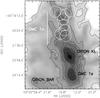 |
Fig. 1 JCMT/SCUBA 850 μm continuum image of the OMC 1 cloud (Johnstone & Bally 1999), with various features indicated as references, such as the Orion Bar, Orion South and Orion KL. The black contours range from 0.5 to 8.5 Jy beam-1 in steps of 2 Jy beam-1, and from 15 to 30 Jy beam-1 in steps of 5 Jy beam-1. The white circles represent the pointings made to cover the SMA area surveyed, and their size corresponds to the SMA primary beam, 55′′. |
The SMA correlator covers 2 GHzbandwidth in each of the two side-bands separated by 10 GHz. Each band is divided into 24 chunksof 104 MHzwidth, which were covered by fine spectral resolution (256 channelscorrespond to a velocity resolution of 0.53 km s-1 in our observing setting). In addition to continuum observations, molecular lines such as CO (2–1), 13CO (2–1),C18O(2–1),and 13CS (5–4),were simultaneously obtained with the 2 GHzbandwidth in each sideband. These molecular line data will be presented in a future article.
The continuum data from the two sidebands (USB + LSB) were combined to obtain a higher signal-to-noiseratio. The combined configurations of the arrays provided projected baselines ranging from 5.1 to 56.0 kλ. Our observations were insensitive to structures larger than 32′′ (13 000 AU/0.07 pc) at the 10% level (Wilner & Welch 1994). Passband calibration was achieved by observing the quasars, 3C 454.3and 3C 273. Amplitudes and phases were calibrated by observations of 0530+135and 0541-056for the compact configurations and 0607-085and 0541-056for the subcompact configurations. These flux densities were determined relative to Uranus. The overall flux uncertainty was estimated to be ~20%. The pointing accuracy of the SMA observations was ~3′′ . The raw data were calibrated using MIR, originally developed for the Owens Valley Radio Observatory (Scoville et al. 1993) and adopted for the SMA.
To produce the mosaic continuum image, certain frequencies (which include the aforementioned molecular lines) were subtracted from the visibility data using the miriad task uvlin. The effective bandwidth for the continuum emission is approximately 3.6 GHz. We used the task CLEAN in miriad with the ROBUST parameter equal to 2, and then we combined the resulting images linearly with the task LINMOS. The final synthesized beam size results directly from combining all observations and is ≈ 3′′ FWHM (corresponding to 1200 AU). The achieved mean rms noise level for the entire mosaic image is estimated to be ≈11 mJy. The SMA observational log for each date and the observational parameters are summarized in Tables 1 and 2.
SMA observational logs.
SMA observational parameters
3. Results
3.1. New compact continuum sources
We detected 24 previously unknown compact millimeter sources within the OMC-1N region; these new sources were identified as having peak fluxes ≥5σ (i.e. ≥55 mJy beam-1) and are shown in Fig. 2. There is fainter extended emission at the 3σ level that may correspond to smaller cores. Only two of these sources were found to have (near- and mid) infrared counterparts; one of them coincides with SMA-10, and the other is located very near SMA-15, more precisely, with the small protrusion extending from the peak of the emission. We also detected red- and/or blueshifted CO emission arising from bipolar outflows.
We used MIRIAD (Sault et al. 1995) to measure the fluxes, sizes, and positions of each source (IMFIT procedure), where each source was modeled by an elliptical 2D Gaussian. As can be seen in Fig. 2, the sources appear to be distributed in groups, that is, they are connected as a single structure when using a 3σ contour. We therefore carried out multi-Gaussian fits so that all sources in a particular group were fit together. Six groups of sources were fit simultaneously: group 1 consists of sources SMA-1 and SMA-2, group 2 consists of sources SMA-4 and SMA-5, group 3 consists of sources SMA-6, SMA-7, SMA-8, SMA-9 and SMA-10, group 4 consists of sources SMA-11, SMA-12, SMA-13 and SMA-14, group 5 consists of sources SMA-17, SMA-18 and SMA-19, and group 6 consists of sources SMA-21 and SMA-22. Figure 2 shows that SMA-15 may in fact consist of two sources (the infrared counterpart offset from the position of the main peak and coincident with the small southwest extended emission supports this), but we were unable to fit SMA-15 with two simultaneous 2D Gaussians. The same is true for source SMA-20. The measured properties for each source are listed in Table 3. The total integrated flux listed was measured from the 2D multi-Gaussian fitting. Sources SMA-9, SMA-11, and SMA-18 are poorly fit by a 2D Gaussian model, but it was necessary to include them to fit the nearby brighter compact source(s) within the same group properly. The errors cited for the total flux correspond to the statistical uncertainties, but they are in fact dominated by the calibration uncertainty that is ~20%, as previously mentioned in Sect. 2. The total flux listed in Table 3 corresponds to thermal dust emission, but may also have some contribution from thermal free-free emission from protostellar jets. To calculate this latter contribution, we used a spectral index of 0.6 (Panagia & Felli 1975; Anglada et al. 1998) and estimated the flux from thermal free-free emission, Sν, for these sources from Sν ∝ ν0.6, where ν is the frequency of the emission. The SMA sources detected in OMC 1n share very similar properties with those in OMC 3 (Takahashi et al. 2013) and OMC 2 (Takahashi et al. 2015). We can therefore make use of VLA measurements at 3.6 cm of OMC 2 protostars (Reipurth et al. 1999,Table 1) as a benchmark, since most of the flux at this wavelength is from free-free emission. Using their lowest and highest flux densities, we find that the contribution of thermal free-free emission from jets would range between 1.1 mJy and 20.9 mJy at 1.3 mm for the OMC 2 sources. We assume that the sources in OMC 1n would have a similar contribution, but future observations are necessary to measure the exact amount of free-free emission for each of the OMC 1n sources. We note that the estimated flux from thermal free-free emission is typically within the error of the total integrated flux for each source.
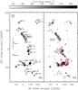 |
Fig. 2 SMA 1.3 mm continuum emission (grayscale, lowest level corresponds to 3σ emission), where the black contours range from 5σ to 10σ in steps of 1σ (σ ~ 11 mJy beam-1). Coordinate offsets are measured with respect to (α,δ) = (05h35m17.0s, −05°22′00.0′′) (J2000.0). In panel a), the new sources are indicated by arrows with their corresponding IDs (compare with Tables 3 and 4). The vertical scale bars correspond to the median first and seventh nearest-neighbor separations of the SMA sources, λobs 1 and λobs 2, respectively (see Sect. 3.3 and Table 5). Panel b) shows CO (2−1) red- and blueshifted emission from molecular outflows in red and blue contours, respectively. The red contour levels range from 14 to 136 Jy beam-1 km s-1 in steps of 14 Jy beam-1 km s-1. The blue contour levels range from 9 to 31 Jy beam-1 km s-1 in steps of 3 Jy beam-1 km s-1. The molecular outflow velocities range from 0 to 40 (redshifted emission) and from −20 to 0 (blueshifted emission). |
Measured observables of the SMA sources from 2D elliptical Gaussian fitting.
Before proceeding, we would like to briefly remark on the nomenclature used in this paper. The terms “core” and ”clump” do not have a strict definition in the field of star formation and are sometimes used interchangeably in the literature, which may lead to erroneous comparisons of results. We use these two terms in the following manner: a core (or several cores) is formed within a clump and is therefore relatively denser than the clump, and we follow the nomenclature used in Takahashi et al. (2013), where “small-scale clumps” in the ∫-shaped-filament are structures with sizes on the order of 0.3−0.1 pc, and “cores” are structures with sizes typically ten times smaller. The aforementioned groups of sources would therefore correspond to small-scale clumps that fragmented into cores; group 1 corresponds to a single small-scale clump that fragmented into two cores, for instance, group 3 corresponds to a single small-scale clump that fragmented into five cores, etc. Each core corresponds to an SMA source.
The left panel of Fig. 3 compares the SMA 1.3 mm sources (grayscale) with previously observed JCMT/SCUBA 850 μm emission (Johnstone & Bally 1999; contours). Our SMA observations spatially resolved all the JCMT/SCUBA clumps, meaning that all of the single-dish identified clumps are associated with at least one SMA source. The right panel of Fig. 3 compares the SMA 1.3 mm sources (grayscale) with previously observed VLA NH3 (1,1) emission (Wiseman & Ho 1998; contours). The SMA sources clearly lie within dense filamentary regions, although they are not always located at the center of an ammonia clump. For example, sources SMA-1 and SMA-2 are located at the center of the same 850 μm clump, but are spatially offset by ~10′′ from the center of an ammonia core. Other sources that are not located near the center of ammonia small-scale clumps are SMA-3, SMA-4, SMA-5, SMA-13, SMA-16, SMA-21, SMA-23, and SMA-24.
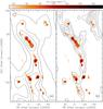 |
Fig. 3 Comparison of SMA continuum emission (grayscale) with: a) 850 μm JCMT emission, where the JCMT contours range from 0.5 to 20 Jy beam-1 in steps of 1 Jy beam-1 (Johnstone & Bally 1999); and b) VLA NH3 (1,1) emission integrated from 4.6 to 12.3 km s-1, where two lowest NH3 contours are 20 and 100 mJy beam-1 km s-1 and the higher level contours continue in steps of 100 mJy beam-1 km s-1 (Wiseman & Ho 1998). Coordinate offsets are measured with respect to (α,δ) = (05h35m17.0s, −05°22′00.0′′) (J2000.0). |
3.2. Masses and sizes
We can determine the masses of these sources if we assume the 1.3 mm emission arises from optically thin dust that can be characterized by a single temperature (e.g., Mundy et al. 1995; Bally et al. 1998). The total gas+dust mass is calculated from the following equation: 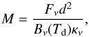 (1)where Fν is the measured total flux of the source, d is the distance to the source, Bν(Td) is the Planck function for a dust temperature Td, and κν is the dust mass opacity. We followed Menten et al. (2007) and adopted a distance of 414 ± 7 pc to the SMA sources. The dust mass opacity was calculated from κν = 0.1(ν/ 1000 GHz)β cm2 g-1 (Beckwith et al. 1990), assuming a gas-to-dust ratio of 100, and where we took the emissivity index, β, to be 1.5, following Johnstone & Bally (1999) and the latest results from Planck for this region (Lombardi et al. 2014); κν is therefore κ230 GHz = 11 × 10-3 cm2 g-1. According to Wiseman & Ho (1998), the filament within which the SMA sources are embedded has a kinetic gas temperature of 15 K, and this is the temperature we assumed for Td in our mass calculation (assuming that the gas and dust temperatures are coupled). Using the integrated flux densities given in Table 3, we calculated the masses for each source, and their values are shown in Table 4. We calculated the radius of each source by taking the geometric mean of the deconvolved major and minor axes (given in Table 3),
  , which in turn was used to determine the number densities,
  , for each source assuming spherical symmetry. Both Rgeom and are shown in Table 4.
Tatematsu et al. (2008) found a constant temperature of ~20 K over the entire ∫-shaped filament. Here we opted for using the temperature measured by Wiseman & Ho (1998) because this value was obtained from higher angular resolution interferometric observations. The single-dish observations from Tatematsu et al. (2008) include extended emission of the cloud that envelopes the small-scale clumps and is presumably warmer, thus providing a slightly higher temperature. This effect is also suggested by Herschel data (e.g., see Fig. 2 of Lombardi et al. 2014). On the other hand, the interferometric observations filtered out the extended emission and should give a more reliable estimate of the temperature of the dense regions within the filament. For comparison purposes we added a note to Table 4 where we show that changing the temperature assumption to 20 K would lower the masses by factor of ~1.5.
Calculated properties of the SMA sources and their nearest-neighbor separation.
3.3. Spatial distribution
Figure 3 shows that the SMA sources are distributed along dense filamentary structures, and part of groups that show a quasi-equal spacing between (and within) them. To better quantitatively describe these spatial scales associated with the SMA sources, we present in Fig. 4 an analysis of the first to tenth (projected) nearest-neighbor separations (NNS). Panel (a) shows the measured median value of the Nth (N = 1, ..., 10) NNS in black vs. their σ-value. The plot shows that the empirical function has two minima that occur for the first and seventh nearest neighbors. A minimum in the σNth NNS function indicates a characteristic spatial scale of the distribution of sources (i.e., the width of the NNS distribution narrows as sources have similar separation values). Panel (b) shows that the distributions of the first nearest-neighbor distribution (open, black line histogram ) peaks at the median value of 6.5′′ with a σ of 4.7′′; the seventh nearest-neighbor distribution (filled, black line histogram) peaks at the median value of 31.5′′ with a σ of 8.8′′2.
To determine if these two distributions correspond to bona fide characteristic spatial scalings of the region, we carried out 10 000 Monte Carlo simulations of a randomly spatially distributed sample of sources, of the same number as our SMA detected sources, and located within an area of the same size. Panel (a) of Fig, 4 shows that the median separations for this randomly spatial distributed sample (red) increases monotonically, presenting only one minimum, for N = 1 (we found that the σNth NNS function for a random distribution always increases monotonically, regardless of the number of sources or the size of the area in which they are distributed). The first NNS for the simulated sample has a median value of 14.0′′ and σ of 8.6′′, which is greater than the homologous measured values by a factor larger than 2. Panel (b) shows that randomly spatial distributed sample presents broad and shallow peaks for their first and seventh nearest-neighbor distributions (red) that cannot describe the narrow well-defined, peaks of the observed distributions of the SMA sources. The two spatial scalings we measure are therefore not random and are a characteristic feature of OMC 1n. We also carried out a two-point correlation function and found positive correlation at the same two spatial scales (see Fig. A.1). We continue our analysis assuming that these spatial scalings are a result of the fragmentation of the parental structures that gave rise to the small-scale clumps and cores in OMC 1n.
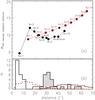 |
Fig. 4 a) Median nth nearest-neighbor separations of the SMA sources vs. σNth NNS, where each data point (black filled symbol) is labeled from N = 1,..., 10.The red symbols represent the median nth NNS for a random spatial distribution for comparison purposes (see text). b) Distribution of the first NNS (open black histogram) and the distribution of the seventh NNS (filled black histogram). The red dashed-line and the red solid-line histograms correspond to the first and seventh NNS for random spatial distributions, respectively. All the histogram bin widths correspond to the approximate SMA synthesized beam size, 3′′. |
4. Discussion
The size and density of the new SMA sources, combined with a general lack of counterpart infrared sources and the presence of CO outflows, indicate that these compact SMA sources are either cores with young protostars in the Class 0 evolutionary phase, or pre-stellar cores. From Takahashi et al. (2013) we know that the compact submillimeter sources in OMC 3 range in masses from 0.3 M⊙ to 5.7 M⊙, and we find in this work that the masses of the OMC 1n sources range between 0.1 M⊙ and 3.0 M⊙. The OMC 3 projected source sizes range from 1400 au to 8200 au, whereas the projected OMC 1n source sizes range from 400 au to 1300 au. In terms of density, sources in OMC 3 have 2.0 × 108 cm-3>nH2> 1.9 × 106 cm-3, while the OMC 1n sources are on average less dense, and have 2.6 × 107 cm-3>nH2> 2.8 × 106 cm-3. Finally, comparison of the fraction of infrared counterparts, 67% for OMC 3 and 8% for OMC 1n, indicates that the latter are less evolved than the former. We find that the OMC 1n sources are indeed very young objects that have not had enough time to substantially move away from their birth site within the filament. Class 0 protostars (≲104 yr; Larson 2003) with an average velocity of 1 km s-1 may travel up to ~0.01 pc away from their birth site during this evolutionary phase. This means that it is valid to infer the fragmentation scale of the parental filament from the measured spatial distribution of these very young sources.
The measured separations are projected distances. The observed scales, λobs, would therefore correspond to the fragmentation scales, λfrag, if the inclination, i, of the filament and small-scale clumps with respect to the line-of-sight is 90° [λobs = λfrag·sin(i)]. As discussed in Sect. 3.3 and shown in Fig. 4, there are two observed spatial scales present in OMC 1n: a larger scale corresponding to λobs_1 = 31′′± 9′′ (0.06 ± 0.02 pc), and a smaller scale corresponding to λobs_2 = 6′′± 5′′ (0.01 ± 0.01 pc). The λobs_1 scale corresponds to the distance between the JCMT/SCUBA dust emission small-scale clumps and to the distance between the VLA NH3 small-scale clumps (see Fig. 3). The λobs_2 scale corresponds to the separation of the new SMA compact sources within these small-scale clumps. The inclination of the OMC 1n filament is unknown. The median inclination of a randomly oriented filament is 60° (Hanawa et al. 1993); using this angle of inclination the fragmentation scales would be λfrag_1=36′′ (0.07 pc) and λfrag_2 = 7′′ (0.01 pc). The projection effect is thus smaller than the error in λobs_1 and λobs_2 for an inclination of 60°. In fact, the projection effect is only significant if the inclination angle is smaller than 50°.
A filament may be supported against gravitational collapse and fragmentation through different physical means, of which we considered the following three: thermal pressure, turbulent pressure, and magnetic pressure. These physical processes may affect the final fragmentation scale of the filament differently. In addition, the kinematics of the filament and small-scale clumps may also affect the spatial distribution of the sources formed therein. The filament could be experiencing large-scale collapse. Within the filament, the small-scale clumps could also be undergoing local collapse. The large-scale collapse of the filament may shorten the distance between the small-scale clumps, and likewise, local collapse of the small-scale clumps may shorten the distance between the cores therein. The measured fragmentation scales may thus indicate which of these aforementioned processes are dominant. We briefly discuss each of these scenarios below.
We first consider at which spatial scales the filament would fragment if no support against gravitational collapse were provided by either turbulence or magnetic fields, that is, if we were to consider only thermal pressure. The Jeans length (Spitzer 1998), λJeans, is given by
 (2)
(2)
where cs is the sound speed given by  (kB is the Boltzmann constant, T is the temperature, μ is the mean molecular weight, and mH is the proton mass), G is the gravitional constant, and ρ0 is the initial volume density given by n0/ (μmH). We calculated the Jeans length of the filament, λJeans_1, by using the peak density of the OMC 1n filament (nH2 ~105 cm-3, Johnstone & Bally 1999) and a temperature of 15 K (Wiseman & Ho 1998). For these conditions the local Jeans length for the filament is 0.08 pc (40′′). For a temperature of 10 K, λJeans_1 = 0.07 pc (35′′). The larger fragmentation scale measured λobs_1 is thus consistent with λJeans_1 for inclination angles greater than 50°. It is therefore possible that the OMC 1n filament underwent thermal fragmentation that generated the small-scale clumps therein. To analyze the fragmentation of the small-scale clumps themselves, we calculated the local Jeans length using Eq. (2), a density of 5 × 105 cm-3 (Wiseman & Ho 1998), and a temperature of 15 K as before: λJeans_2 = 0.033 pc (16′′). For a temperature of 10 K (canonical value of the temperature of a dense pre-stellar region, i.e., a region that has not yet undergone internal heating), λJeans_2 = 0.026 pc (13′′). The measured separation between individual cores within the small-scale clumps λobs_2 is smaller than λJeans_2 by a factor of ~2−3. The measured spatial lengths and Jeans lengths are summarized in Table 5.
Summary of measured spatial scales and corresponding local Jeans lengths.
For comparison, our previous SMA study of the OMC 3 region in the ∫-shapedfilament (Takahashi et al. 2013) detected 12 spatially resolved continuum sources at 850 μm. We measured a quasi-periodic separation between these individual sources of ~17′′ (0.035 pc). This spatial scale is smaller than the local thermal Jeans length by a factor of 2.0−7.3.
Our finding – a two-level hierarchical fragmentation in OMC 1n – generally agrees with studies in other star-forming regions, notably in the Spokes cluster in NGC 2264 (Teixeira et al. 2006, 2007), in the more massive infrared dark cloud IRDC G11.11-0.12 (Kainulainen et al. 2013), and in other massive star-forming regions (Palau et al. 2015). Further observational evidence for this type of fragmentation is given in a recent study of the young stellar population of the Orion A and B clouds, where Megeath et al. (2016) found that the median separation between sources is similar to the Jeans length. In all these aforementioned regions, the respective fragmentation lengths observed are consistent with the local spherical Jeans length for spatial scales smaller than 0.5 pc. For spatial scales larger than 0.5 pc, Kainulainen et al. (2013) found that the observed fragmentation scale is consistent with the prediction from the gravitational instability of a self-gravitating isothermal cylinder (e.g., Nagasawa 1987). We explore next which physical processes could explain the smaller fragmentation length measured in OMC1 1n from the separations of the individual cores.
Turbulence will produce a fragmentation scale larger than the Jeans length, as discussed in Takahashi et al. (2013). Theoretical fragmentation length scales are directly proportional to the sound speed, cs. Turbulence can be included in this calculation by using an effective sound speed, ceff, instead of cs; ceff is given by  , where Δvt and Δvnt correspond to the thermal and non-thermal velocity linewidths, respectively. Turbulence is included in the Δvnt term. In the presence of turbulence, ceff>cs and the fragmentation scale is consequently larger than the thermal Jeans length. Since the two measured fragmentation scales, λobs_1 and λobs_2, are either equal to or smaller than their respective local Jeans lengths, we can rule out turbulence pressure as a dominant physical process in the fragmentation of the filament and small-scale clumps and conclude that it has essentially decayed for these size scales (<0.3 pc) in OMC 1n. This conclusion is consistent with that previously reached by Houde et al. (2009), who found that turbulence does not dominate the dynamics in OMC 1. Takahashi et al. (2013) also ruled out turbulence as a dominant physical process in the fragmentation of OMC 3 and further suggested that it has dissipated for size scales ≤1 pc.
We next discuss possible role of the magnetic field in the fragmentation of OMC 1n. Several polarimetric observations indicate that the magnetic field in OMC 1n is mostly perpendicular to the filament and its small-scale clumps, namely, far-infrared observations at 100 μm from the Kuiper Airborne Observatory (Schleuning 1998), submillimeter observations from CSO at 350 μm (Schleuning 1998; Houde et al. 2004), and JCMT observations at 760 μm (Vallée & Bastien 1999). The orientation of the magnetic field relative to the axis of the filamentary cloud has important implications in terms of its stability (e.g., Nagasawa 1987). Stodólkiewicz (1963) found that the critical length of perturbation increases with increasing magnetic field intensity for the idealized case of a magnetic field perpendicular to an infinitely long cylinder of compressible gas. Assuming the orientation of the larger magnetic field is preserved for smaller scales in the filament (Li et al. 2009) and that the intensity of the magnetic field increases for smaller scales, it follows that the magnetic field topology of OMC 1n cannot explain why λobs_2 is smaller than λJeans_2 (Table 5). Regarding the strength of the magnetic field, B, Houde et al. (2004) calculated a total magnitude of B ≈ 850 μG using the observed line-of-sight magnetic field strength of 360 μG determined from Zeeman detection in CN Crutcher (1999) and an inclination of 65° (consistent with a plane-of-the-sky magnetic field strength of 760 μG determined from polarimetric observations Houde et al. 2009). They concluded that OMC 1 is magnetically supercritical. The mass-to-flux ratio in units of the critical mass-to-flux ratio, γ, (Crutcher 2004) is given by
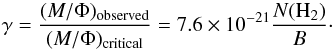 (3)
(3)
Using the aforementioned value of B and an N(H2) of 5 × 1023 cm-2 obtained from Herschel observations (Lombardi et al. 2014), we calculate γ to be ≈4.5, and confirm that OMC 1n is magnetically supercritical. Houde et al. (2004) also calculated a magnetic-to-gravitational energy ratio of ≈0.26. Our current data do not allow us to analyze the magnetic field properties in more detail, but from the above arguments it appears that the magentic field does not provide enough support against gravitational collapse, nor does it explain the shorter separations between cores observed in the small-scale clumps.
After ruling out turbulence and the magnetic field as responsible agents for the smaller fragmentation scales measured in OMC 1n, λobs_2, we now explore other possible processes. As already discussed, thermal fragmentation alone cannot fully explain λobs_2, but if thermal fragmentation were to occur concomitantly with the local collapse of the small-scale clumps, the separations between the individual sources formed within the small-scale clumps are naturally expected to decrease. Pon et al. (2011) showed that local collapse proceeds on a much smaller timescale than global collapse for filamentary structures. This analytical model would be consistent with the scenario where the local collapse in the small-scale clumps occurs at a much faster pace than the global collapse of OMC 1n, thus the shortening of the distances between sources would be more pronounced within the small-scale clumps and not in between them. We propose this may indeed be an important mechanism at play in OMC 1n. We plan to explore this scenario and constrain the effect that local vs. global collapse has on the final spatial separations of the sources with future ALMA data.
5. Summary
We briefly summarize the main results of this paper as follows:
-
1.
We found 24 new compact millimeter sources in OMC 1n that are very likely young protostars in the Class 0 evolutionary phase or pre-stellar objects.
-
2.
The OMC 1n sources range in size from 400 au to 1300 au and in mass from 0.1 M⊙ to 2.3 M⊙ (assuming a dust temperature of 15 K and a distance to OMC 1n of 414 pc). These measured values are lower limits because our data lack the zero spacing flux emitted by more extended structures.
-
3.
The spatial distribution of the sources reveal a hierarchical two-level fragmentation of the parental filamentary structure − the larger scale, λobs_1 = 31′′± 9′′ (0.06 ± 0.02 pc), is associated with the fragmentation of the filament into small-scale clumps, while the smaller scale, λobs_2 = 6′′± 5′′ (0.01 ± 0.01 pc), is associated with the fragmentation of the small-scale clumps into cores/SMA sources.
-
4.
Comparison of these two measured scales with the local Jeans lengths of the parental filament and of the small-scale clumps showed that the larger observed scale, λobs_1, is consistent with thermal fragmentation for inclinations greater than 50°. The smaller scale, λobs_2, is smaller than the local Jeans lengths of the parental small-scale clumps by a factor of ~2−3.
-
5.
We discussed other mechanisms that may explain the smaller measured scale, λobs_2. Further molecular line data are needed to distinguish the different physical processes involved, such as local collapse within OMC 1n.
The SMA is a joint project between the SAO and the Academia Sinica Institute of Astronomy and Astrophysics and is funded by the Smithsonian Institution and the Academia Sinica.
For a sample of sources that excludes SMA-9, -12, and -18, we find that the first NNS has a median value of 7.6′′ with a σ of 4.3′′, and the seventh NNS has a median value of 38.6′′ and a corresponding σ of 9.4′′. Although the measured parameters of these sources have larger error bars (cf. Table 3), they are fully consistent with the statistical trend of the other sources.
Acknowledgments
The authors gratefully acknowledge the anonymous referee for their constructive review of an earlier version of this manuscript. P.S.T. is very grateful for support from the Joint ALMA Observatory (Santiago, Chile) Science Visitor Programme while visiting co-author S. Takahashi. The authors wish to thank Jennifer Wiseman and Doug Johnstone for kindly sharing with us their VLA NH3 and JCMT/SCUBA 850 μm data, respectively, and for constructive comments. We would also like to thank Phil Myers, Josep Miquel Girart, Aina Palau, Andy Pon, Álvaro Hacar and Oliver Czoske for insightful discussions. We thank all the SMA staff members for making these observations possible. The authors wish to recognize and acknowledge the very significant cultural role and reverence that the summit of Mauna Kea has always had within the indigenous Hawaiian community. We are most fortunate to have the opportunity to conduct observations from this mountain. P.S.T. also wishes to thank Alvin C. Inja for positive interaction during the writing of this manuscript.
References
- André, P., Men’shchikov, A., Bontemps, S., et al. 2010, A&A, 518, L102 [NASA ADS] [CrossRef] [EDP Sciences] [Google Scholar]
- Anglada, G., Villuendas, E., Estalella, R., et al. 1998, AJ, 116, 2953 [NASA ADS] [CrossRef] [Google Scholar]
- Bally, J., Lanber, W. D., Stark, A. A., & Wilson, R. W. 1987, ApJ, 312, L45 [NASA ADS] [CrossRef] [Google Scholar]
- Bally, J., Testi, L., Sargent, A., & Carlstrom, J. 1998, AJ, 116, 854 [NASA ADS] [CrossRef] [Google Scholar]
- Beckwith, S. V. W., Sargent, A. I., Chini, R. S., & Guesten, R. 1990, AJ, 99, 924 [NASA ADS] [CrossRef] [Google Scholar]
- Crutcher, R. M. 1999, ApJ, 520, 706 [NASA ADS] [CrossRef] [Google Scholar]
- Crutcher, R. M. 2004, The Magnetized Interstellar Medium, 123 [Google Scholar]
- Hacar, A., Tafalla, M., Kauffmann, J., & Kovács, A. 2013, A&A, 554, A55 [NASA ADS] [CrossRef] [EDP Sciences] [Google Scholar]
- Hanawa, T., Nakamura, F., Matsumoto, T., et al. 1993, ApJ, 404, L83 [NASA ADS] [CrossRef] [Google Scholar]
- Heitsch, F. 2013, ApJ, 769, 115 [NASA ADS] [CrossRef] [Google Scholar]
- Ho, P. T. P., Moran, J. M., & Lo, K. Y. 2004, ApJ, 616, L1 [NASA ADS] [CrossRef] [Google Scholar]
- Houde, M., Dowell, C. D., Hildebrand, R. H., et al. 2004, ApJ, 604, 717 [NASA ADS] [CrossRef] [Google Scholar]
- Houde, M., Vaillancourt, J. E., Hildebrand, R. H., Chitsazzadeh, S., & Kirby, L. 2009, ApJ, 706, 1504 [NASA ADS] [CrossRef] [Google Scholar]
- Ivezić, Ż., Connolly, A., VanderPlas, J., & Gray, A. 2013, Statistics, Data Mining, and Machine Learning in Astronomy, eds. Ż. Ivezić et al. (Princeton University Press) [Google Scholar]
- Johnstone, D., & Bally, J. 1999, ApJ, 510, L49 [NASA ADS] [CrossRef] [Google Scholar]
- Kainulainen, J., Ragan, S. E., Henning, T., & Stutz, A. 2013, A&A, 557, A120 [NASA ADS] [CrossRef] [EDP Sciences] [Google Scholar]
- Kirk, H., Myers, P. C., Bourke, T. L., et al. 2013, ApJ, 766, 115 [NASA ADS] [CrossRef] [Google Scholar]
- Landy, S. D., & Szalay, A. S. 1993, ApJ, 412, 64 [NASA ADS] [CrossRef] [Google Scholar]
- Larson, R. B. 2003, Rep. Prog. Phys., 66, 1651 [NASA ADS] [CrossRef] [Google Scholar]
- Li, H.-b., Dowell, C. D., Goodman, A., Hildebrand, R., & Novak, G. 2009, ApJ, 704, 891 [NASA ADS] [CrossRef] [Google Scholar]
- Lombardi, M., Bouy, H., Alves, J., & Lada, C. J. 2014, A&A, 566, A45 [NASA ADS] [CrossRef] [EDP Sciences] [Google Scholar]
- Megeath, S. T., Gutermuth, R., Muzerolle, J., et al. 2016, AJ, 151, 5 [NASA ADS] [CrossRef] [Google Scholar]
- Menten, K. M., Reid, M. J., Forbrich, J., & Brunthaler, A. 2007, A&A 474, 515 [NASA ADS] [CrossRef] [EDP Sciences] [Google Scholar]
- Muench, A., Getman, K., Hillenbrand, L., & Preibisch, T. 2008, Handbook of Star Forming Regions, 483 [Google Scholar]
- Mundy, L. G., Looney, L. W., & Lada, E. A. 1995, ApJ, 452, L137 [NASA ADS] [CrossRef] [Google Scholar]
- Myers, P. C. 2009, ApJ, 700, 1609 [NASA ADS] [CrossRef] [EDP Sciences] [Google Scholar]
- Myers, P. C. 2011, ApJ, 735, 82 [NASA ADS] [CrossRef] [Google Scholar]
- Nagasawa, M. 1987, Prog. Theoret. Phys., 77, 635 [Google Scholar]
- O’Dell, C. R. 2001, A&A&A, 39, 99 [Google Scholar]
- O’Dell, C. R., Muench, A., Smith, N., & Zapata, L. 2008, Handbook of Star Forming Regions, 544 [Google Scholar]
- Ostriker, J. 1964, ApJ, 140, 1056 [NASA ADS] [CrossRef] [MathSciNet] [Google Scholar]
- Palau, A., Ballesteros-Paredes, J., Vázquez-Semadeni, E., et al. 2015, MNRAS, 453, 3785 [NASA ADS] [CrossRef] [Google Scholar]
- Panagia, N., & Felli, M. 1975, A&A, 39, 1 [NASA ADS] [Google Scholar]
- Peterson, D. E., & Megeath, S. T. 2008, Handbook of Star Forming Regions, 590 [Google Scholar]
- Pineda, J. E., & Teixeira, P. S. 2013, A&A, 555, A106 [NASA ADS] [CrossRef] [EDP Sciences] [Google Scholar]
- Pon, A., Johnstone, D., & Heitsch, F. 2011, ApJ, 740, 88 [NASA ADS] [CrossRef] [Google Scholar]
- Reipurth, B., Rodríguez, L. F., & Chini, R. 1999, AJ, 118, 983 [NASA ADS] [CrossRef] [Google Scholar]
- Sault, R. J., Teuben, P. J., & Wright, M. C. H. 1995, Astronomical Data Analysis Software and Systems IV, 77, 433 [Google Scholar]
- Schleuning, D. A. 1998, ApJ, 493, 811 [NASA ADS] [CrossRef] [Google Scholar]
- Schneider, S., & Elmegreen, B. G. 1979, ApJS, 41, 87 [NASA ADS] [CrossRef] [Google Scholar]
- Schneider, N., Csengeri, T., Bontemps, S., et al. 2010, A&A, 520, A49 [NASA ADS] [CrossRef] [EDP Sciences] [Google Scholar]
- Scoville, N. Z., Carlstrom, J. E., Chandler, C. J., et al. 1993, PASP, 105, 1482 [NASA ADS] [CrossRef] [Google Scholar]
- Spitzer, L. 1998, Physical Processes in the Interstellar Medium (Wiley-VCH), 335 [Google Scholar]
- Stodólkiewicz, J. S. 1963, Acta Astron., 13, 30 [NASA ADS] [Google Scholar]
- Tackenberg, J., Beuther, H., Henning, T., et al. 2014, A&A, 565, A101 [NASA ADS] [CrossRef] [EDP Sciences] [Google Scholar]
- Takahashi, S., Ho, P. T. P., Teixeira, P. S., Zapata, L. A., & Su, Y.-N. 2013, ApJ, 763, 57 [NASA ADS] [CrossRef] [Google Scholar]
- Tatematsu, K., Kandori, R., Umemoto, T., & Sekimoto, Y. 2008, PASJ, 60, 407 [NASA ADS] [Google Scholar]
- Teixeira, P. S., Lada, C. J., Young, E. T., et al. 2006, ApJ, 636, L45 [NASA ADS] [CrossRef] [Google Scholar]
- Teixeira, P. S., Zapata, L. A., & Lada, C. J. 2007, ApJ, 667, L179 [NASA ADS] [CrossRef] [Google Scholar]
- Vallée, J. P., & Bastien, P. 1999, ApJ, 526, 819 [NASA ADS] [CrossRef] [Google Scholar]
- VanderPlas, J., Connolly, A. J., Ivezic, Z., & Gray, A. 2012, Proc. Conf. on Intelligent Data Understanding (CIDU), 47, 47 [Google Scholar]
- Wilner, D. J., & Welch, W. J. 1994, ApJ, 427, 898 [NASA ADS] [CrossRef] [Google Scholar]
- Wiseman, J. J., & Ho, P. T. P. 1998, ApJ, 502, 676 [NASA ADS] [CrossRef] [Google Scholar]
- Zapata, L. A., Rodríguez, L. F., Kurtz, S. E., O’Dell, C. R., & Ho, P. T. P. 2004, ApJ, 610, L121 [NASA ADS] [CrossRef] [Google Scholar]
Appendix A: Additional spatial correlation analysis
We also perfomed a two-point correlation analysis of the spatial distribution of the SMA sources, using the Landy & Szalay (1993) estimator. The correlation function, ω(θ), is therefore given by 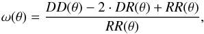 (A.1)where DD(θ) corresponds to the distribution of measured angular separations, θ, between pairs of SMA sources.
RR(θ) corresponds to the distribution of angular separations between pairs of random sources, and DR(θ) corresponds to the distribution of angular separations between pairs of an SMA source and a random source. The sample of random sources consisted of the same number of sources as the sample of SMA sources, placed within the same RA and Dec ranges, and was generated 10 000 times; the final RR(θ) and DR(θ) distributions were averaged along θ.
Figure A.1 shows that ω(θ) has two maxima, denoting preferred spatial correlations at separations consistent with λobs_1 and λobs_2, as measured above using the median first and seventh nearest-neighbor separations of the SMA sources, respectively.
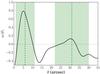 |
Fig. A.1 Correlation function, ω(θ), of the angular separation, θ, between the SMA sources. The vertical dashed lines correspond to λobs_1 and λobs_2, respectively. The width of the shaded areas correspond to the corresponding error of λobs_1 and λobs_2. The dotted horizontal marks ω(θ) = 0. |
All Tables
All Figures
|
Fig. 1 JCMT/SCUBA 850 μm continuum image of the OMC 1 cloud (Johnstone & Bally 1999), with various features indicated as references, such as the Orion Bar, Orion South and Orion KL. The black contours range from 0.5 to 8.5 Jy beam-1 in steps of 2 Jy beam-1, and from 15 to 30 Jy beam-1 in steps of 5 Jy beam-1. The white circles represent the pointings made to cover the SMA area surveyed, and their size corresponds to the SMA primary beam, 55′′. |
| In the text | |
|
Fig. 2 SMA 1.3 mm continuum emission (grayscale, lowest level corresponds to 3σ emission), where the black contours range from 5σ to 10σ in steps of 1σ (σ ~ 11 mJy beam-1). Coordinate offsets are measured with respect to (α,δ) = (05h35m17.0s, −05°22′00.0′′) (J2000.0). In panel a), the new sources are indicated by arrows with their corresponding IDs (compare with Tables 3 and 4). The vertical scale bars correspond to the median first and seventh nearest-neighbor separations of the SMA sources, λobs 1 and λobs 2, respectively (see Sect. 3.3 and Table 5). Panel b) shows CO (2−1) red- and blueshifted emission from molecular outflows in red and blue contours, respectively. The red contour levels range from 14 to 136 Jy beam-1 km s-1 in steps of 14 Jy beam-1 km s-1. The blue contour levels range from 9 to 31 Jy beam-1 km s-1 in steps of 3 Jy beam-1 km s-1. The molecular outflow velocities range from 0 to 40 (redshifted emission) and from −20 to 0 (blueshifted emission). |
| In the text | |
|
Fig. 3 Comparison of SMA continuum emission (grayscale) with: a) 850 μm JCMT emission, where the JCMT contours range from 0.5 to 20 Jy beam-1 in steps of 1 Jy beam-1 (Johnstone & Bally 1999); and b) VLA NH3 (1,1) emission integrated from 4.6 to 12.3 km s-1, where two lowest NH3 contours are 20 and 100 mJy beam-1 km s-1 and the higher level contours continue in steps of 100 mJy beam-1 km s-1 (Wiseman & Ho 1998). Coordinate offsets are measured with respect to (α,δ) = (05h35m17.0s, −05°22′00.0′′) (J2000.0). |
| In the text | |
|
Fig. 4 a) Median nth nearest-neighbor separations of the SMA sources vs. σNth NNS, where each data point (black filled symbol) is labeled from N = 1,..., 10.The red symbols represent the median nth NNS for a random spatial distribution for comparison purposes (see text). b) Distribution of the first NNS (open black histogram) and the distribution of the seventh NNS (filled black histogram). The red dashed-line and the red solid-line histograms correspond to the first and seventh NNS for random spatial distributions, respectively. All the histogram bin widths correspond to the approximate SMA synthesized beam size, 3′′. |
| In the text | |
|
Fig. A.1 Correlation function, ω(θ), of the angular separation, θ, between the SMA sources. The vertical dashed lines correspond to λobs_1 and λobs_2, respectively. The width of the shaded areas correspond to the corresponding error of λobs_1 and λobs_2. The dotted horizontal marks ω(θ) = 0. |
| In the text | |
Current usage metrics show cumulative count of Article Views (full-text article views including HTML views, PDF and ePub downloads, according to the available data) and Abstracts Views on Vision4Press platform.
Data correspond to usage on the plateform after 2015. The current usage metrics is available 48-96 hours after online publication and is updated daily on week days.
Initial download of the metrics may take a while.