| Issue |
A&A
Volume 586, February 2016
|
|
|---|---|---|
| Article Number | A30 | |
| Number of page(s) | 9 | |
| Section | Stellar structure and evolution | |
| DOI | https://doi.org/10.1051/0004-6361/201527454 | |
| Published online | 22 January 2016 | |
Magnetic field topology of τ Scorpii
The uniqueness problem of Stokes V ZDI inversions⋆
1 Department of Physics and Astronomy, Uppsala University, Box 516, 75120 Uppsala, Sweden
e-mail: Oleg.Kochukhov@physics.uu.se
2 Department of Physics, Royal Military College of Canada, PO Box 17000, Station “Forces”, Kingston, ON K7K 7B4, Canada
Received: 25 September 2015
Accepted: 24 November 2015
Context. The early B-type star τ Sco exhibits an unusually complex, relatively weak surface magnetic field. Its topology was previously studied with the Zeeman Doppler imaging (ZDI) modelling of high-resolution circular polarisation (Stokes V) observations.
Aims. Here we assess the robustness of the Stokes V ZDI reconstruction of the magnetic field geometry of τ Sco and explore the consequences of using different parameterisations of the surface magnetic maps.
Methods. This analysis is based on the archival ESPaDOnS high-resolution Stokes V observations and employs an independent ZDI magnetic inversion code.
Results. We succeeded in reproducing previously published magnetic field maps of τ Sco using both general harmonic expansion and a direct, pixel-based representation of the magnetic field. These maps suggest that the field topology of τ Sco is comprised of comparable contributions of the poloidal and toroidal magnetic components. At the same time, we also found that available Stokes V observations can be successfully fitted with restricted harmonic expansions, by either neglecting the toroidal field altogether, or linking the radial and horizontal components of the poloidal field as required by the widely used potential field extrapolation technique. These alternative modelling approaches lead to a stronger and topologically more complex surface field structure. The field distributions, which were recovered with different ZDI options, differ significantly and yield indistinguishable Stokes V profiles but different linear polarisation (Stokes Q and U) signatures.
Conclusions. Our investigation underscores the well-known problem of non-uniqueness of the Stokes V ZDI inversions. For the magnetic stars with properties similar to τ Sco (relatively complex field, slow rotation) the outcome of magnetic reconstruction strongly depends on the adopted field parameterisation, rendering photospheric magnetic mapping and determination of the extended magnetospheric field topology ambiguous. Stokes Q and U spectropolarimetric observations represent the only way of breaking the degeneracy of surface magnetic field models.
Key words: stars: atmospheres / stars: early-type / stars: magnetic field / stars: individual:τScorpii
© ESO, 2016
1. Introduction
Tomographic inversion of spectral time series observations of stars (referred to as Doppler imaging) is an important modern tool for the characterisation of stellar surface structure. Since these methods were introduced in the 1970s to reconstruct the chemical abundance spot distributions of Ap stars (Khokhlova 1976), their use has been extended to map temperature inhomogeneities of cool stars (e.g. Vogt & Penrod 1983), surface velocity fields of pulsating stars (Kochukhov 2004), and stellar surface magnetic fields (Donati & Semel 1990; Brown et al. 1991; Piskunov & Kochukhov 2002), the latter with the acquisition of spectropolarimetric, rather than spectral, time series.
The basic principles underlying Doppler imaging approaches are rotational modulation in combination with indirect (i.e. spectral) resolution of the stellar surface. The latter is achieved through exploitation of the rotational Doppler broadening of spectral line profiles, combined with the temporal evolution of the profile.
Because Doppler imaging relies on the inversion of a spectral time series to reconstruct a 2D surface map, it is inherently ill-posed in most of its implementations. As a consequence, significant efforts have been invested to understand the accuracy and uniqueness of the resulting maps (e.g. Rice 1991; Rice & Strassmeier 2000). In the reconstruction of stellar magnetic fields (known as Zeeman Doppler imaging, or ZDI), an important focus has been to understand the uniqueness of maps that have been obtained from spectropolarimetric time series where the Stokes vector has not been fully characterised (e.g. Donati & Brown 1997; Kochukhov & Piskunov 2002; Rosén & Kochukhov 2012). This problem potentially affects most magnetic maps reconstructed using ZDI, as the large majority are inferred from inversion of only Stokes I and V spectra, i.e. without knowledge of the Stokes Q and U linear polarisation parameters.
Donati et al. (2006, hereafter D06), reported the discovery of a medium-strength (~0.5 kG) magnetic field on the young, massive star τ Sco (B0.2 V, HR 6165, HD 149438). Circularly polarised Zeeman signatures, modulated according to the ~41 d rotational period of the star, were clearly detected in observations that were collected mostly using the ESPaDOnS spectropolarimeter. Using a ZDI approach, D06 reconstructed the large-scale structure of the magnetic topology of τ Sco, finding a magnetic structure that was unusually complex for a hot star, with significant power in spherical-harmonic modes up to degree 5. The surface topology they recovered is dominated by a potential field, although they concluded that a moderate toroidal component is probably also present. They also extrapolated the reconstructed surface magnetic field into the region above the stellar surface using a potential, force-free assumption. The topology of the extended magnetic field that they derived is also more complex than a global dipole and features, in particular, a significantly warped torus of closed magnetic loops that encircle the star, with additional, smaller, networks of closed field lines. Donati & Landstreet (2009) have published an updated model of the surface field using a more extensive data set.
Ignace et al. (2010) observed τ Sco using the Suzaku X-ray observatory. Based on the potential field extrapolation of D06, two main X-ray eclipses were expected at phases of around 0.3 and 0.8, in conjunction with enhanced UV line absorptions that were observed at those times (D06). While the Suzaku pointings include phases close to those at which the eclipses were predicted, no X-ray variations anywhere near the expected amplitudes were detected. The lack of X-ray eclipses likely implies that the X-ray formation region is located significantly further away from the star than is predicted according to the ZDI reconstruction and potential extrapolation of D06.
To better understand the origin of this discrepancy, we have investigated the uniqueness of the surface magnetic map of τ Sco that was derived from the Stokes V time series of D06. In particular, we have assessed the sensitivity of the ZDI reconstruction to the choice of parameterisation of the stellar surface magnetic field distribution.
The rest of the paper is organised as follows. In Sect. 2 we discuss spectropolarimetric observations of τ Sco and summarise alternative approaches to parameterisation of the surface magnetic field in ZDI. Section 3 presents magnetic maps obtained using various surface field parameterisations and assesses the consequence of these differences for the magnetic energy distribution at different spatial scales and for the magnetospheric field structure. The results of our study are summarised and discussed in Sect. 4.
2. Methods
2.1. Spectropolarimetric observational data
We employed the same collection of CFHT ESPaDOnS observations of τ Sco as was used by Donati & Landstreet (2009), apart from the addition of a single additional observation acquired in July 2009. This observation corresponds to phase 0.740 (a phase at which an earlier observation already exists).
All observations were extracted from the CFHT Archive in reduced form, and normalised to the continuum order-by-order using polynomial fits. Least-squares deconvolution (LSD) was applied to each spectrum using the ilsd procedure, as implemented by Kochukhov et al. (2010). We used a line mask based on a Vienna Atomic Line Database (vald, Kupka et al. 1999) “Extract Stellar” request, retaining only lines stronger than 10% of the continuum, cleaned and adjusted in depth to best match the observed spectrum of τ Sco.
All extracted profiles were scaled corresponding to a Landé factor of 1.20, an unbroadened central depth of 0.2, and a wavelength of 500 nm. Observations from the same nights were averaged and one low signal-to-noise ratio (S/N) spectrum was excluded, resulting in a data set that comprises 49 rotational phases.
2.2. Parameterisation of magnetic maps in ZDI
2.2.1. Direct parameterisation
Early Zeeman Doppler imaging studies (Brown et al. 1991; Piskunov & Kochukhov 2002) treated each component of the surface magnetic field vector distribution as an independent two-dimensional map, defined on a discrete longitude-latitude grid. Each of the three magnetic field component maps were simultaneously fitted to spectropolarimetric time series data, employing one or another form of regularisation (e.g. maximum entropy or Tikhonov methods). This approach to the stellar magnetic field mapping, hereafter called direct inversion, results in magnetic field distributions that do not necessarily satisfy Maxwell’s equations. In particular, the net signed flux through the stellar surface can significantly deviate from zero.
Other, less obvious problems of the direct field parameterisation approach include various degeneracies and cross-talks between different magnetic field components when ZDI is based only on the Stokes V spectra (Brown et al. 1991; Kochukhov & Piskunov 2002; Rosén & Kochukhov 2012). Moreover, the choice of regularisation applied in the direct ZDI problem appears to be critical for adequate reconstruction of certain types of globally-organised magnetic field topologies. For instance, according to Brown et al. (1991) and Donati (2001), direct ZDI that is guided by the maximum entropy constraint fails to recover a simple dipolar field configuration, even using spectra in all four Stokes parameters. Conversely, the ZDI that employs Tikhonov regularisation succeeds in reconstructing dipolar and low-order multipolar fields (Piskunov & Kochukhov 2002; Kochukhov & Piskunov 2002).
2.2.2. General spherical-harmonic parameterisation
Spherical-harmonic expansion is an alternative form of the stellar magnetic field parameterisation favoured by the more recent ZDI studies (Donati 2001; Donati et al. 2006; Kochukhov et al. 2014). In this method the free parameters of the magnetic inversion problem are coefficients specifying amplitudes of various spherical-harmonic modes. The most general form of the harmonic representation of an arbitrary surface vector field distribution is given by ![\begin{align} B_{\rm r} (\theta, \phi) &= -\sum_{\ell=1}^{\ell_{\rm max}} \sum_{m=-\ell}^{\ell} \alpha_{\ell,m} Y_{\ell,m} (\theta, \phi), \label{eq1} \\ B_{\theta} (\theta, \phi) &= -\sum_{\ell=1}^{\ell_{\rm max}} \sum_{m=-\ell}^{\ell} \left[\beta_{\ell,m} Z_{\ell,m} (\theta, \phi) + \gamma_{\ell,m} X_{\ell,m} (\theta,\phi) \right], \label{eq2} \\ B_{\phi} (\theta, \phi) &= -\sum_{\ell=1}^{\ell_{\rm max}} \sum_{m=-\ell}^{\ell}\left[\beta_{\ell,m} X_{\ell,m} (\theta, \phi) - \gamma_{\ell,m} Z_{\ell,m} (\theta,\phi) \right], \label{eq3} \end{align}](/articles/aa/full_html/2016/02/aa27454-15/aa27454-15-eq7.png) where Yℓ,m(θ,φ), Zℓ,m(θ,φ), and Xℓ,m(θ,φ) are spherical-harmonic functions of the angular degree ℓ and azimuthal order m and their derivatives with respect to the latitude θ and longitude φ (see Kochukhov et al. 2014 for definitions of these quantities). The coefficients αℓ,m and βℓ,m characterise, respectively, the vertical and horizontal components of the poloidal (potential) field. The γℓ,m coefficients specify the strength of the toroidal (non-potential) field components.
where Yℓ,m(θ,φ), Zℓ,m(θ,φ), and Xℓ,m(θ,φ) are spherical-harmonic functions of the angular degree ℓ and azimuthal order m and their derivatives with respect to the latitude θ and longitude φ (see Kochukhov et al. 2014 for definitions of these quantities). The coefficients αℓ,m and βℓ,m characterise, respectively, the vertical and horizontal components of the poloidal (potential) field. The γℓ,m coefficients specify the strength of the toroidal (non-potential) field components.
It is easy to see several attractive features of the ZDI based on the harmonic field description. This representation of the field structure automatically obeys the requirement of zero total magnetic flux piercing through the closed surface (one of Maxwell’s equations). It also enables detailed quantitative characterisation of ZDI results by making it straightforward to, e.g., assess the strength of the poloidal vs. toroidal field components or axisymmetric vs. non-axisymmetric field. It was also claimed by Donati (2001) that the spherical-harmonic parameterisation alleviates to some extent the problem of the radial/meridional field cross-talk in the ZDI with Stokes V data alone.
2.2.3. Constrained spherical-harmonic parameterisation
The description of the surface magnetic field geometry in terms of the general harmonic expansion given by Eqs. (0)–(2) carries along a large number of degrees of freedom, which may be superfluous for particular ZDI problems. For example, the necessity of including the toroidal field components given by the coefficients γℓ,m is not always explicitly justified by ZDI studies. On the other hand, using independent sets of the αℓ,m and βℓ,m coefficients implies independent treatment of the horizontal and vertical poloidal field components, which appears to be unnecessary, e.g. in the context of studies of the magnetic field topologies of early-type stars (Landstreet & Mathys 2000; Bagnulo et al. 2002).
In addition to simplicity arguments, there are fundamental physical reasons to expect a link between αℓ,m and βℓ,m. The method of potential source surface field (PSSF) extrapolation (Jardine et al. 2002, 2013) is frequently used to analyse the extended magnetospheric field topology based on the photospheric ZDI map of the radial field component. It was applied to τ Sco by D06. This technique imposes a relation between αℓ,m and βℓ,m for a given location of the source surface Rs. For example, with the definitions of Kochukhov et al. (2013) and the stellar radius R⋆, one can determine 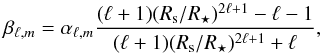 (4)which reduces to the condition βℓ,m ≈ αℓ,m when Rs ≫ R⋆.
Somewhat surprisingly, despite a wide-spread application of the PSSF extrapolations of ZDI results, almost all magnetic mapping studies (with the exception of Hussain et al. 2002) do not attempt to incorporate this constraint into the magnetic inversions themselves. As discussed by Jardine et al. (2013), this leads to an inconsistency between the poloidal horizontal field that is reconstructed by ZDI and the horizontal field that is calculated using the PSSF technique. The ZDI maps of τ Sco and corresponding field extrapolation presented by D06 also suffer from this inconsistency.
2.3. Application of magnetic inversions to τ Sco
The main goal of our study is to explore the sensitivity of the ZDI modelling of τ Sco to different forms of magnetic field parameterisation. To this end, we have carried out Stokes V magnetic inversions using the direct field parameterisation (Model 1), the general harmonic parameterisation (γℓ,m ≠ 0, βℓ,m ≠ αℓ,m, Model 2), and two constrained harmonic field representations. Specifically, we tested the feasibility of fitting the circular polarisation observations of τ Sco with a purely poloidal field (γℓ,m = 0, βℓ,m ≠ αℓ,m, Model 3) and with a mixture of toroidal and constrained poloidal fields (γℓ,m ≠ 0, βℓ,m = αℓ,m, Model 4). For the relatively complex field of τ Sco and its source surface radius of Rs = 1.8–2.0 R⋆ (D06, Petit et al. 2013), the latter parameterisation is essentially equivalent to the application of Eq. (4). In all inversions discussed below, the spherical-harmonic expansion was truncated to ℓ = 10. Similar to D06, we found that none of the models with ℓ ≤ 2 can produce an acceptable fit to the data.
Reconstruction of the magnetic field topology of τ Sco was carried out with the help of the InversLSD ZDI code described by Kochukhov et al. (2013). The Tikhonov regularisation (Tikhonov & Arsenin 1977) was applied for the direct inversion (Model 1); a penalty function minimising the energy of high-order modes (Kochukhov et al. 2013) was employed to constrain the harmonic inversions (Models 2−4). Since no detectable variability is seen in Stokes I, only the Stokes V LSD profiles were modelled.
We adopted a projected rotational velocity of vesini = 6 km s-1 and an inclination angle of i = 70° following D06. The local Stokes V profile shape was approximated with the Unno-Rachkovsky analytical solution of the polarised radiative transfer equation in the Milne-Eddington atmosphere (Landi Degl’Innocenti & Landolfi 2004). For these calculations the Zeeman splitting pattern of the average line was represented by a triplet with the same effective Landé factor g0 = 1.2 and wavelength λ0 = 500 nm, as were adopted for normalisation of the observed LSD profiles. The depth and width of the theoretical local profile were adjusted to match the observed Stokes I LSD line shape.
3. Results
Summary of ZDI inversions for τ Sco.
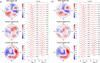 |
Fig. 1 Global magnetic field topology of τ Sco derived with ZDI inversions for the case of a) direct parameterisation of the magnetic maps (Model 1) and b) harmonic parameterisation with βℓ,m ≠ αℓ,m,γℓ,m ≠ 0 (Model 2). In each panel the left column shows the flattened polar projection of the radial, meridional, and azimuthal field components. The colour bar indicates the field strength in kG. The observed (thin black line) and computed (thick red line) LSD Stokes V profiles are compared on the right side of each panel. The profiles are offset vertically according to the rotational phase indicated next to each spectrum. |
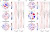 |
Fig. 2 Same as Fig. 1 for the harmonic ZDI inversions with a) βℓ,m ≠ αℓ,m,γℓ,m = 0 (Model 3) and b) βℓ,m = αℓ,m,γℓ,m ≠ 0 (Model 4). |
3.1. Magnetic field distributions
Results of the ZDI inversions based on different surface field parameterisations are summarised in Table 1. For each inversion, this table gives a measure of the quality of the final fit to the observed Stokes V LSD profiles, the rms values of the three magnetic field components, the total magnetic energy, and an estimate of the relative energy contributions of the poloidal/toroidal and axisymmetric/non-axisymmetric field components.
The resulting magnetic field maps and corresponding line profile fits are presented in Figs. 1 and 2. For each ZDI model, these figures illustrate the radial, meridional, and azimuthal field distributions over the surface of τ Sco in the flattened polar projection, which is similar to the presentation used by D06.
The inversions that correspond to Model 1 (direct ZDI) and 2 (general spherical-harmonic ZDI) are shown in Fig. 1. Evidently, these magnetic field maps are very similar in all three magnetic vector components. There is no evidence that reliance on a spherical-harmonic expansion leads to an appreciably different field distribution, despite an additional physical constraint. We conclude that for τ Sco the effective degrees of freedom in the direct and harmonic inversions are largely equivalent.
A comparison of Fig. 1 with the magnetic field distribution published by D06 and with an updated magnetic field map of τ Sco presented by Donati & Landstreet (2009) shows an excellent agreement. Both details of the surface distributions of the individual field components and their amplitudes agree well. Very small remaining differences may be related to a different local Stokes V profile shape that was adopted in the two studies.
Despite this encouraging concordance of the magnetic maps themselves, their interpretation is somewhat different. D06 reported that the potential field contribution clearly dominates, in terms of the magnetic energy, over the toroidal field, although both are required to fit the observations. Instead, we found that the toroidal field is slightly stronger than the poloidal contribution. The importance of the toroidal field is confirmed by Fig. 3, which presents the horizontal field maps separately for the poloidal and toroidal components of the field distribution that corresponds to Model 2. It is clear that the non-potential field components dominate for both the meridional and azimuthal field maps.
We cannot offer a definitive explanation for the discrepancy in the interpretation of essentially the same magnetic map obtained here and by D06. In our analysis the energy of each spherical-harmonic field component was established by the direct integration of the corresponding  maps over the stellar surface. The same approach was used by D06 (P. Petit, priv. comm.). We have verified that restricting the magnetic inversion to the same rotational phases as used by D06 does not change the inferred relative magnetic energy contributions of the poloidal and toroidal field components.
Results of the ZDI with the constrained spherical-harmonic expansions are presented in Fig. 2. Both Model 3 and 4 yield an acceptable fit to the observed Stokes V profiles, which is only marginally worse than the fits achieved by Models 1 and 2. In comparison, D06 reported a significantly worse fit with a purely poloidal field topology than with a poloidal plus toroidal field configuration. These authors did not consider the constrained harmonic field parameterisation equivalent to our Model 4.
In our inversions, a good fit with constrained harmonic expansions is achieved at the expense of making the field stronger and more complex. In particular, the ZDI inversion. which ignores the toroidal field (Model 3), recovers local field strengths of up to 1.2 kG and has a total energy 2.3–2.5 times that of Models 1 and 2. The radial field distribution seen in Fig. 2a is somewhat reminiscent of the field structure shown in Fig. 1. At the same time, the horizontal field topology is entirely different.
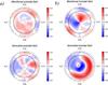 |
Fig. 3 Comparison of the a) poloidal and b) toroidal contributions to the horizontal magnetic field obtained in the general harmonic ZDI inversion (Model 2), illustrated in Fig. 1b. |
An even stronger field is required to obtain an adequate description of the observations when the toroidal field is present but the horizontal and radial poloidal fields are assumed to be linked (αℓ,m = βℓ,m, Model 4). Both the radial and horizontal components of the resulting field distribution are significantly different from those obtained before; the maximum local surface field strength exceeds 2.5 kG and the total magnetic energy is now almost 20 times higher, compared to Models 1 and 2.
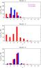 |
Fig. 4 Distribution of magnetic energy over different harmonic modes for ZDI inversions 2–4. The energy of poloidal components (light bars) is compared with toroidal contribution (dark bars) at different angular degree ℓ. |
3.2. Magnetic energy spectrum
In addition to the assessment of the total poloidal/toroidal component contributions, reported in Table 1, we analysed a distribution of the magnetic field energy over different ℓ-modes for all inversions based on the spherical-harmonic expansion. The fractional energy in different poloidal and toroidal modes is illustrated in Fig. 4. For Model 2 (general harmonic parameterisation), the poloidal field is spread over ℓ = 1–4, while the toroidal field peaks at ℓ = 2–3. For Model 3 (purely poloidal field), the energies are spread over the range ℓ = 1–6, with ℓ = 4 providing the maximum contribution. For Model 4 (linked horizontal and vertical components of the poloidal field), both the poloidal and toroidal fields are dominated by the contribution from ℓ = 3–4 modes. The lowest order, dipolar, contribution is also much smaller for Model 4 compared to other ZDI inversions. To summarise, the spatial magnetic energy spectrum inferred by the Stokes V ZDI depends sensitively on the harmonic parameterisation of the surface magnetic field.
3.3. Potential field extrapolation
As mentioned in Sect. 2.2.3, ZDI maps of the stellar surface magnetic fields are often used as the basis for studying the extended magnetospheric field topology with the help of the potential field extrapolation methods. Here we have applied the PSSF extrapolation technique, described by Jardine et al. (2002, 2013), to the radial field component of each ZDI map that we have derived for τ Sco. The same source surface radius of R = 2 R⋆ as used by D06 was adopted for all extrapolations. A 3D rendering of the magnetic field lines for the magnetospheric field structures, which correspond to different ZDI maps, is presented in Fig. 5. We omitted the extrapolation for Model 1 from this figure since it is very similar to Model 2.
Analysis of Fig. 5 suggests that excluding the toroidal field from ZDI reconstruction (Model 3) has a relatively small impact on the magnetospheric field topology. However, some difference is seen for the rotational phase 0.5: the field structure extrapolated from the ZDI map of Model 3 exhibits additional field loops at the disk centre.
On the other hand, the extended field topology, which corresponds to Model 4, is entirely different from the results obtained for Models 2 and 3. The extended field is more complex, especially at phases 0.50 and 0.75. One may expect that the variability of the X-ray emission, which is due to the material trapped in this particular magnetospheric geometry, will differ from the emission that corresponds to the magnetospheric structures of Models 2 and 3. We emphasise again that, unlike the other two PSSF extrapolations presented in Fig. 5, the extended field structure of Model 3 is self-consistent with the respective ZDI map.
4. Conclusions and discussion
In this study we have carried out a detailed investigation of the reliability of the Stokes V ZDI reconstruction of the surface magnetic field topology for the early-B star τ Sco. Specifically, we have fitted the observed circular polarisation profile time series, employing different forms of the surface magnetic map parameterisation, and have compared the resulting surface distributions in terms of their geometry, magnetic energy, and boundary condition for the potential field extrapolation. The main findings of our investigation are as follows:
-
The ZDI with general harmonic parametrisation gives a verysimilar result to the direct ZDI inversion constrained with theTikhonov regularisation. Thus, for the relatively complexmagnetic field topology of τ Sco, the harmonicparameterisation does not offer any advantages over the directinversion in terms of overcoming biases and cross-talks typical ofthe Stokes V ZDI reconstructions.
-
The magnetic field map obtained with the general harmonic ZDI inversion is fully consistent with the results published by Donati et al. (2006) and Donati & Landstreet (2009). At the same time, contrary to these authors, we found that the energy of the toroidal field component is comparable, if not larger, than the poloidal one.
-
We were able to successfully fit the available Stokes V time series with two types of restricted harmonic fields. On the one hand, the observations can be acceptably reproduced by ignoring the toroidal field altogether. On the other hand, a fit with the toroidal field plus a poloidal contribution with coupled vertical and horizontal vector components, as required by the potential field extrapolation technique, is also feasible.
-
The ZDI models derived in our study successfully reproduce the Stokes V profile variability with a static magnetic field geometry and no differential rotation. This implies that the field was stable on the time scale of five years that was covered by the available spectropolarimetric observations.
The three ZDI maps obtained using alternative forms of the harmonic field parameterisation are significantly different in terms of their topological details and the average field strength. They also yield somewhat different distributions of the magnetic energy as a function of the spherical-harmonic angular degree ℓ and a different extended magnetospheric field structure according to the PSSF extrapolation method. At the same time, these field maps yield essentially indistinguishable theoretical Stokes V profiles. We interpret this as another manifestation of the uniqueness problems, which have been discussed extensively by previous ZDI studies (Donati & Brown 1997; Kochukhov & Piskunov 2002; Rosén & Kochukhov 2012), and which are associated with the limited information content of the Stokes V time series.
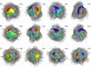 |
Fig. 5 Magnetospheric magnetic field topology of τ Sco obtained by extrapolating ZDI surface magnetic field maps. Each row shows results for a) Model 2; b) Model 3; and c) Model 4. In each case the star is shown at four rotational phases, as indicated above each panel. |
The noticeable increase of the reconstructed field strength and complexity from Model 3 (no toroidal field) to Model 4 (coupled vertical and horizontal poloidal field components) suggests that the latter degree of freedom is more important for ZDI than the mere presence or absence of the toroidal field. While many ZDI studies pondered the latter aspect, none has tried to physically interpret the fact that the best-fitting ZDI maps often require a different magnitude and even an opposite sign for the vertical and horizontal components of the same spherical-harmonic terms. At least in the case of stable, fossil magnetic fields of early-type stars, a physical motivation for such geometries is absent. The only existing detailed theoretical models of fossil field geometries (Braithwaite & Nordlund 2006; Braithwaite 2008) match the stellar field to the vacuum exterior condition, implying the same coupling of the vertical and horizontal harmonic terms as assumed in our ZDI Model 4.
It is obvious (e.g. see Table 1) that attaining the same fit quality with restricted harmonic field parameterisations requires a significantly stronger field than in the case of the ZDI with general spherical-harmonic expansion (Model 2). One can, therefore, insist that the latter map should be preferred based on the simplicity or minimum energy argument. However, this reasoning ignores the physical nature of the problem, which for early-type stars requires a consistent field topology all the way from the stellar surface to the circumstellar environment. This consistency is achieved by Model 4 but not by Models 2 or 3. Nevertheless, we emphasise that simplicity or physical arguments aside, the available Stokes V observational data by itself definitely excludes ℓ = 1−2 models but cannot provide a distinction between the three high-order harmonic field topologies.
Extending spectropolarimetric observations to linear polarisation (Stokes Q and U parameters) provides a promising way to distinguish degenerate harmonic field models. Figure 6 compares theoretical Stokes Q and U time series for all four ZDI magnetic maps that we derived in our paper. It is clear that the profiles of Models 1 and 2 are still virtually indistinguishable since they correspond to essentially identical surface maps. On the other hand, the predicted Q and U profiles of Models 2 and 3 are different in all but a few rotational phases. Furthermore, the strong-field Model 4 yields a high-amplitude linear polarisation signal that is straightforward to distinguish from Models 2 and 3. Thus, it appears that linear spectropolarimetry is critical for solving the problem of non-uniqueness in the Stokes V ZDI modelling of τ Sco. Unfortunately, a comparison of several Stokes Q and U observations of this star available in the ESPaDOnS archive with the ZDI model predictions is currently inconclusive: the observations do not have a sufficient S/N to test the models using single spectral lines, and the use of higher precision Stokes Q/U LSD profiles for such a test requires more sophisticated modelling (see Rosén et al. 2015), which is beyond the scope of this paper.
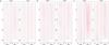 |
Fig. 6 Comparison of the synthetic LSD Stokes QU profiles predicted by different ZDI inversions. In each panel the dashed line shows the linear polarisation profiles for Model 2. The solid lines correspond to a) Model 1; b) Model 3; and c) Model 4. The Stokes QU spectra are shown for the same set of rotational phases as the Stokes V profiles in Figs. 1 and 2. |
Finally, we wish to comment that the Stokes V ZDI modelling of τ Sco is significantly complicated by the slow rotation of this star. In this case, the rotational Doppler broadening is comparable to the local line profile width and therefore the spatial Doppler resolution is ineffective when compared to fast rotators, which are usually targeted by Doppler imaging. As demonstrated by Fig. 7, if the projected rotational velocity of τ Sco were to be several times larger than its vesini = 6 km s-1, one could easily discern the Stokes V profiles of Model 4 from the time series of the two other harmonic maps. Models 2 and 3, however, still yield nearly identical Stokes V profiles for this fictitious fast-rotating τ Sco analog.
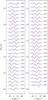 |
Fig. 7 Synthetic Stokes V profiles that correspond to the magnetic field distributions of Model 2 (solid line), Model 3 (dotted line), and Model 4 (dash-dotted line) for the projected rotational velocity of vesini = 50 km s-1. |
Details of the surface magnetic field geometry of τ Sco, in particular the relative strengths of its poloidal and toroidal field components, have important implications for the theoretical understanding of massive star magnetism. The fields in these stars are believed to be fossil remnants from an earlier evolutionary phase. Magnetohydrodynamical (MHD) simulations of the transition of an initially random fossil field to a stable configuration were carried out by Braithwaite & Nordlund (2006) and Braithwaite (2008). They demonstrated that, to maintain stability on stellar evolutionary time-scales, the interior field must have a mixed poloidal-toroidal configuration. However, these MHD models do not anticipate the presence of a significant toroidal field component at the stellar surface. In this context, the confirmation of these types of fields at the surface of τ Sco would represent a major challenge for the current theoretical models, which possibly hints at the operation of some physical mechanism other than a simple fossil field relaxation.
To summarise our study, a Stokes V ZDI inversion is significantly uncertain for a star that, like τ Sco, rotates slowly and exhibits a complex, non-dipolar surface magnetic field. Some key characteristics of the surface field topology (the presence of toroidal field, major geometrical features, typical field strength, degree of complexity, etc.) cannot be reliably ascertained from first principles. An assessment of these characteristics requires a strong assumption to be made (equivalently, choosing one of several possible surface field parameterisations) about the field without an overly compelling physical reason. Obtaining Stokes Q and U observations and incorporating these data in ZDI inversions represents the only generic solution to this problem.
Acknowledgments
O.K. acknowledges financial support from the Knut and Alice Wallenberg Foundation, the Swedish Research Council, and the Göran Gustafsson Foundation. G.A.W. is supported by a Discovery Grant from the Natural Science and Engineering Research Council (NSERC) of Canada.
References
- Bagnulo, S., Landi Degl’Innocenti, M., Landolfi, M., & Mathys, G. 2002, A&A, 394, 1023 [NASA ADS] [CrossRef] [EDP Sciences] [Google Scholar]
- Braithwaite, J. 2008, MNRAS, 386, 1947 [NASA ADS] [CrossRef] [Google Scholar]
- Braithwaite, J., & Nordlund, Å. 2006, A&A, 450, 1077 [NASA ADS] [CrossRef] [EDP Sciences] [Google Scholar]
- Brown, S. F., Donati, J.-F., Rees, D. E., & Semel, M. 1991, A&A, 250, 463 [NASA ADS] [Google Scholar]
- Donati, J.-F. 2001, in Astrotomography, Indirect Imaging Methods in Observational Astronomy, eds. H. M. J. Boffin, D. Steeghs, & J. Cuypers (Berlin: Springer Verlag), Lect. Notes Phys., 573, 207 [Google Scholar]
- Donati, J.-F., & Brown, S. F. 1997, A&A, 326, 1135 [NASA ADS] [Google Scholar]
- Donati, J.-F., & Landstreet, J. D. 2009, ARA&A, 47, 333 [NASA ADS] [CrossRef] [MathSciNet] [Google Scholar]
- Donati, J.-F., & Semel, M. 1990, Sol. Phys., 128, 227 [NASA ADS] [CrossRef] [Google Scholar]
- Donati, J.-F., Howarth, I. D., Jardine, M. M., et al. 2006, MNRAS, 370, 629 [NASA ADS] [CrossRef] [Google Scholar]
- Hussain, G. A. J., van Ballegooijen, A. A., Jardine, M., & Collier Cameron, A. 2002, ApJ, 575, 1078 [NASA ADS] [CrossRef] [Google Scholar]
- Ignace, R., Oskinova, L. M., Jardine, M., et al. 2010, ApJ, 721, 1412 [NASA ADS] [CrossRef] [Google Scholar]
- Jardine, M., Wood, K., Collier Cameron, A., Donati, J.-F., & Mackay, D. H. 2002, MNRAS, 336, 1364 [NASA ADS] [CrossRef] [Google Scholar]
- Jardine, M., Vidotto, A. A., van Ballegooijen, A., et al. 2013, MNRAS, 431, 528 [NASA ADS] [CrossRef] [Google Scholar]
- Khokhlova, V. L. 1976, Soviet. Astron., 19, 576 [Google Scholar]
- Kochukhov, O. 2004, ApJ, 615, L149 [NASA ADS] [CrossRef] [Google Scholar]
- Kochukhov, O., & Piskunov, N. 2002, A&A, 388, 868 [NASA ADS] [CrossRef] [EDP Sciences] [Google Scholar]
- Kochukhov, O., Makaganiuk, V., & Piskunov, N. 2010, A&A, 524, A5 [NASA ADS] [CrossRef] [EDP Sciences] [Google Scholar]
- Kochukhov, O., Mantere, M. J., Hackman, T., & Ilyin, I. 2013, A&A, 550, A84 [NASA ADS] [CrossRef] [EDP Sciences] [Google Scholar]
- Kochukhov, O., Lüftinger, T., Neiner, C., Alecian, E., & MiMeS Collaboration 2014, A&A, 565, A83 [NASA ADS] [CrossRef] [EDP Sciences] [Google Scholar]
- Kupka, F., Piskunov, N., Ryabchikova, T. A., Stempels, H. C., & Weiss, W. W. 1999, A&AS, 138, 119 [NASA ADS] [CrossRef] [EDP Sciences] [MathSciNet] [PubMed] [Google Scholar]
- Landi Degl’Innocenti, E., & Landolfi, M. 2004, Polarization in Spectral Lines (Kluwer Academic Publishers), Astrophys. Space Sci. Libr., 307 [Google Scholar]
- Landstreet, J. D., & Mathys, G. 2000, A&A, 359, 213 [NASA ADS] [Google Scholar]
- Petit, V., Owocki, S. P., Wade, G. A., et al. 2013, MNRAS, 429, 398 [NASA ADS] [CrossRef] [Google Scholar]
- Piskunov, N., & Kochukhov, O. 2002, A&A, 381, 736 [NASA ADS] [CrossRef] [EDP Sciences] [Google Scholar]
- Rice, J. B. 1991, A&A, 245, 561 [NASA ADS] [Google Scholar]
- Rice, J. B., & Strassmeier, K. G. 2000, A&AS, 147, 151 [NASA ADS] [CrossRef] [EDP Sciences] [Google Scholar]
- Rosén, L., & Kochukhov, O. 2012, A&A, 548, A8 [NASA ADS] [CrossRef] [EDP Sciences] [Google Scholar]
- Rosén, L., Kochukhov, O., & Wade, G. A. 2015, ApJ, 805, 169 [NASA ADS] [CrossRef] [Google Scholar]
- Tikhonov, A. N., & Arsenin, V. Y. 1977, Solution of Ill-posed Problems (New York: Wiley) [Google Scholar]
- Vogt, S. S., & Penrod, G. D. 1983, in IAU Colloq. 71: Activity in Red-Dwarf Stars, eds. P. B. Byrne, & M. Rodono, Astrophys. Space Sci. Libr., 102, 379 [Google Scholar]
All Tables
All Figures
|
Fig. 1 Global magnetic field topology of τ Sco derived with ZDI inversions for the case of a) direct parameterisation of the magnetic maps (Model 1) and b) harmonic parameterisation with βℓ,m ≠ αℓ,m,γℓ,m ≠ 0 (Model 2). In each panel the left column shows the flattened polar projection of the radial, meridional, and azimuthal field components. The colour bar indicates the field strength in kG. The observed (thin black line) and computed (thick red line) LSD Stokes V profiles are compared on the right side of each panel. The profiles are offset vertically according to the rotational phase indicated next to each spectrum. |
| In the text | |
|
Fig. 2 Same as Fig. 1 for the harmonic ZDI inversions with a) βℓ,m ≠ αℓ,m,γℓ,m = 0 (Model 3) and b) βℓ,m = αℓ,m,γℓ,m ≠ 0 (Model 4). |
| In the text | |
|
Fig. 3 Comparison of the a) poloidal and b) toroidal contributions to the horizontal magnetic field obtained in the general harmonic ZDI inversion (Model 2), illustrated in Fig. 1b. |
| In the text | |
|
Fig. 4 Distribution of magnetic energy over different harmonic modes for ZDI inversions 2–4. The energy of poloidal components (light bars) is compared with toroidal contribution (dark bars) at different angular degree ℓ. |
| In the text | |
|
Fig. 5 Magnetospheric magnetic field topology of τ Sco obtained by extrapolating ZDI surface magnetic field maps. Each row shows results for a) Model 2; b) Model 3; and c) Model 4. In each case the star is shown at four rotational phases, as indicated above each panel. |
| In the text | |
|
Fig. 6 Comparison of the synthetic LSD Stokes QU profiles predicted by different ZDI inversions. In each panel the dashed line shows the linear polarisation profiles for Model 2. The solid lines correspond to a) Model 1; b) Model 3; and c) Model 4. The Stokes QU spectra are shown for the same set of rotational phases as the Stokes V profiles in Figs. 1 and 2. |
| In the text | |
|
Fig. 7 Synthetic Stokes V profiles that correspond to the magnetic field distributions of Model 2 (solid line), Model 3 (dotted line), and Model 4 (dash-dotted line) for the projected rotational velocity of vesini = 50 km s-1. |
| In the text | |
Current usage metrics show cumulative count of Article Views (full-text article views including HTML views, PDF and ePub downloads, according to the available data) and Abstracts Views on Vision4Press platform.
Data correspond to usage on the plateform after 2015. The current usage metrics is available 48-96 hours after online publication and is updated daily on week days.
Initial download of the metrics may take a while.