| Issue |
A&A
Volume 586, February 2016
|
|
|---|---|---|
| Article Number | A151 | |
| Number of page(s) | 16 | |
| Section | Stellar structure and evolution | |
| DOI | https://doi.org/10.1051/0004-6361/201526944 | |
| Published online | 10 February 2016 | |
To Ba or not to Ba: Enrichment in s-process elements in binary systems with WD companions of various masses
1 Institut d’Astronomie et d’Astrophysique, Université Libre de Bruxelles, CP 226, Boulevard du Triomphe, 1050 Brussels, Belgium
e-mail: tmerle@ulb.ac.be
2 Institute of Astronomy, University of Cambridge, Madingley Road, Cambridge CB3 0HA, UK
3 Instituut voor Sterrenkunde, Katholieke Universiteit Leuven, Celestijnenlaan 200D, 3200 Heverlee, Belgium
Received: 12 July 2015
Accepted: 16 October 2015
Context. The enrichment in s-process elements of barium stars is known to be due to pollution by mass transfer from a companion formerly on the thermally pulsing asymptotic giant branch (AGB), now a carbon-oxygen white-dwarf (WD).
Aims. We are investigating the relationship between the s-process enrichment in the barium star and the mass of its WD companion. It is expected that helium WDs, which have masses lower than about 0.5 M⊙ and never reached the AGB phase, should not pollute their giant companion with s-process elements. Therefore the companion should never turn into a barium star.
Methods. Spectra with a resolution of R ~ 86 000 were obtained with the HERMES spectrograph on the 1.2 m Mercator telescope for a sample of 11 binary systems involving WD companions of various masses. We used standard 1D local thermodynamical equilibrium MARCS model atmospheres coupled with the Turbospectrum radiative-transfer code that is embedded in the BACCHUS pipeline to derive the atmospheric parameters through equivalent widths of Fe i and Fe ii lines. Least-squares minimization between the observed and synthetic line shape was used to derive the detailed chemical abundances of CNO and s-process elements.
Results. The abundances of s-process elements for the entire sample of 11 binary stars were derived homogeneously. The sample encompasses all levels of overabundances: from solar [s/ Fe] = 0 to 1.5 dex in the two binary systems with S-star primaries (for which dedicated MARCS model atmospheres were used). The primary components of binary systems with a WD more massive than 0.5 M⊙ are enriched in s-process elements. We also found a trend of increasing [s/Fe] with [C/Fe] or [(C+N)/Fe].
Conclusions. Our results confirm the expectation that binary systems with WD companions less massive than 0.5 M⊙ do not host barium stars.
Key words: stars: abundances / white dwarfs / stars: late-type / binaries: spectroscopic
© ESO, 2016
1. Introduction
The puzzle of the barium stars, a class of K giants with overabundances of heavy elements produced by the s-process of nucleosynthesis (Bidelman & Keenan 1951), has been solved by McClure et al. (1980), who unravelled the binary nature of these stars, and made it clear that the companion is responsible for the heavy-element synthesis. This solution of course requires the companion to be a carbon-oxygen white dwarf (WD), which synthesized the heavy elements while on the thermally pulsing asymptotic giant branch (TP-AGB). An indirect argument supporting this hypothesis has been provided by McClure & Woodsworth (1990) and Jorissen et al. (1998) in the form of the mass-function distribution, which is consistent with the companion masses peaking at 0.6 M⊙, as expected for carbon-oxygen WDs. It is only quite recently that a clear direct argument was presented by Gray et al. (2011) in the form of UV excess flux from these systems detected by GALEX that is attributable to a warm WD. Earlier studies by Schindler et al. (1982), Dominy & Lambert (1983), Böhm-Vitense et al. (1984, 2000), Jorissen et al. (1996), and Frankowski & Jorissen (2006) found similar evidence, although somewhat less convincingly or for a smaller set.
With the advent of sensitive far-UV and X-ray satellites such as EUVE, XMM-Newton, and ROSAT, many warm WDs were discovered from their X-ray or UV flux (see Bilíková et al. 2010, and references therein). Some of them are members of binary systems involving a late-type primary star (e.g. Landsman et al. 1993; Vennes et al. 1995, 1997, 1998; Jeffries & Smalley 1996; Jorissen et al. 1996; Christian et al. 1996; Burleigh et al. 1997, 1998; Hoard et al. 2007; Bilíková et al. 2010), with the latter thus being barium-star candidates. Of course, for this to occur, the progenitor of the current WD had to be a TP-AGB star with an atmosphere enriched in s-process elements. This in turn requires that the s-process nucleosynthesis operated in the H- and He-burning intershell region and that the s-process material was dredged up to the surface. The currently available sample of WDs in binary systems offers an interesting way to test the above paradigm, especially when the mass of the WD is known. By checking whether or not the current companion of the WD is enriched in s-process elements, we may trace the operation of s-process and dredge-up in the AGB progenitor of the current WD. Since its mass is equivalent to the AGB core mass at the end of its evolution, we may thus set constraints on models of AGB evolution by investigating whether there is a threshold on the WD mass for its companion to become a barium star. It is expected for instance that He WDs, which are less massive than CO WDs, had progenitors that did not ascend the AGB. Their companions should thus never be barium stars. This was recently proven to be true for the IP Eri system, whose K primary star, companion of a He WD, is not a barium star (Merle et al. 2014). The present paper addresses this question on a larger sample of binaries involving WDs covering a broad range of masses.
The paper is organized as follows. Section 2 describes the stellar sample and Sect. 3 the observations. Section 4 presents the method used for deriving the atmospheric parameters, and Sect. 5 the resulting abundances, separately for CNO and s-process elements. Sections 6 and 7 contain the discussion of these results and our conclusions.
2. Sample
The binary systems we selected have WD components orbiting a cool star (with Teff< 7000 K). The main selection criterion was the availability of the WD mass, which ranges from 0.3 to 1.0 M⊙. Our sample is listed in Table 1. The sample also covers a broad range of orbital periods and eccentricities. The WD masses are taken from the references listed in Table 1.
Sample of binary systems with a WD companion and known orbital elements.
Here follow remarks on some targets of our sample.
IP Eri (HD 18131) consists of a K0 IV star and a He WD companion. Its evolutionary history has been studied by Siess et al. (2014), and an abundance study was performed by Merle et al. (2014).
14 Aur C (HD 33959) is member of a quadruple system whose component A is a δ Scuti star. 14 Aur C is located 14.6 arcsec from A, at a distance of 104 ± 32 pc from the Sun (van Leeuwen 2007). Spectral types F2V+DA (Vennes et al. 1998) or F5V (Gray et al. 2003) have been proposed. It appears to be a fast rotator. We derived for this star vsini = 16 km s-1. No atmospheric parameters are available yet in the literature for that star. The orbital period of only 3 d makes the dwarf star 14 Aur C an outlier in the period distribution of giant barium stars, but not in that of dwarf carbon stars (if 14 Aur C is one such), where at least one star with a similar period is known (HE 0024-2523 has a period of 3.4 d; Lucatello et al. 2003).
V1261 Ori (HD 35155) is a symbiotic S star (Ake et al. 1991; Jorissen et al. 1996).
IT Vir (HD 121447) is a border case between barium and S stars, since it has been classified as SC2 (Ake 1979), K4Ba (Abia & Wallerstein 1998), K7Ba, and S0.
ζ Cap (HD 204075) is a prototype barium star.
DR Dra (HD 160538) and V1379 Aql (HD 185510) have strong emission cores in the Ca ii H and K lines (Fig. 1), indicative of chromospheric activity related to rapid rotation, as confirmed by our analysis (vsini = 8.5 km s-1 and 18 km s-1, respectively; see Fig. 3) in agreement with the results of Fekel et al. (1993). Emission is also visible in the IR Ca ii triplet.
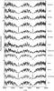 |
Fig. 1 Ca II H and K lines for the sample stars. For comparison, the spectra of the Sun and Arcturus are plotted at the bottom and top of the figure, respectively. Evidence of activity is present in 63 Eri, IP Eri, V1379 Aql, DR Dra, and 56 Peg. |
3. Observations
High-resolution spectra (R ~ 86000) were obtained using the HERMES spectrograph (Raskin et al. 2011) operating at the 1.2 m telescope Mercator at La Palma (Canary Islands, Spain). The HERMES spectrograph is a fiber-fed echelle spectrograph that provides a full spectral coverage from 377 to 900 nm. All the spectra were reduced using the HERMES pipeline software and have a typical signal-to-noise ratio of about 200. The observations were carried out between June 2009 and September 2014.
4. Atmospheric parameters
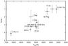 |
Fig. 2 Surface gravity vs. effective temperature for the sample stars. |
First guesses for the atmospheric parameters were determined from previous works (as listed in Sect. 2), from photometry or spectral classification. We assumed the metallicity to be solar to start with [the solar abundance set from Grevesse et al. (2007) is used throughout this paper, in particular with A⊙(Fe) = 7.451].
The atmospheric parameters were then determined iteratively using the pipeline BACCHUS developed by one of the authors (TMa; see also Jofre et al. 2014). This pipeline is based on the 1D local thermodynamical equilibrium (LTE) spectrum-synthesis code Turbospectrum (Alvarez & Plez 1998; Plez 2012) and the method for deriving the atmospheric parameters is based on the fit of the equivalent widths of Fe i and Fe ii lines. The code automatically derives the effective temperature Teff, the logarithmic surface gravity log g, the global metallicity [Fe/H], and the microturbulent velocity ξ by removing any trend in the [Fe/H] vs. χ and [Fe/H] vs. W/λ relations (where χ is the energy of the lower level of a line, W the measured equivalent width, and λ the wavelength of the considered line), and by forcing lines of Fe i and Fe ii to yield the same abundance. We used MARCS model atmospheres (Gustafsson et al. 2008) and a line list constructed from the VALD3 database (Kupka et al. 2011), complemented for Fe and V lines by data from Den Hartog et al. (2014b,a) and Ruffoni et al. (2014).
Spectroscopic stellar parameters derived with BACCHUS.
The synthetic spectra were convolved with a Gaussian function with a σ varying from 6 to 12 km s-1 to match the stellar macroturbulence and/or HERMES resolution. Only reduced equivalent widths (W/λ) of Fe i and Fe ii lines lower than 0.025 are retained in the analysis. For the fast rotators 14 Aur C (Vsini = 16 km s-1) and V1379 Aql (Vsini = 18 km s-1) we convolved the synthetic spectra with a rotational profile.
C, N, and O abundances.
Merle et al. (2014) performed an abundance analysis of IP Eri and obtained the following atmospheric parameters: Teff = 4960 ± 100 K, log g = 3.3 ± 0.3, and [Fe/H]= + 0.09 ± 0.08, which are used here as well.
The atmospheric parameters of the prototypical Ba star ζ Cap (Teff = 5397 ± 82 K, log g = 1.48 ± 0.16, and [Fe/H] = −0.14 ± 0.10) were derived by Prugniel et al. (2011). They were rederived in the present study, and the two parameter sets are similar to each other.
For the two S stars (IT Vir and V1261 Ori) the atmospheric parameters cannot be derived with BACCHUS because strong molecular lines blend many Fe lines and prevent using their equivalent widths. Instead, for V1261 Ori, we adopted the parameters derived by Neyskens et al. (2015), who took the specific chemical composition of S stars and its feedback on the model-atmosphere structure into account. A new grid of MARCS model atmospheres dedicated to S stars (Van Eck et al. 2011) has been used for that purpose. Neyskens et al. (2015) obtained Teff = 3600 K, log g = 1.0, [Fe/H] = −0.5, C/O = 0.5, and [s/Fe] = + 1.0. These parameters are adopted here.
For IT Vir, a border case between Ba and S stars, Abia & Wallerstein (1998) estimated the atmospheric parameters to be Teff = 4000 K, log g = 1.0, and [Fe/H] = −1.0 with ξ = 2 km s-1 and C/O = 0.95, while Smith (1984) had previously found Teff = 4200 K, log g = 0.8, [Fe/H] = 0.05, and C/O= 0.79. The V−K index (V−K = 3.65) combined with the calibration of Bessell et al. (1998) yields Teff = 3900 K. We adopted this value for the temperature combined with the gravity reported by Abia & Wallerstein (1998).
The resulting atmospheric parameters are shown in Table 2, sorted by increasing effective temperatures (as in all the following tables). The uncertainties on the atmospheric parameters provided by the BACCHUS pipeline are those resulting from the propagation of the line-to-line Fe-abundance scatter on the trends used to derive the atmospheric parameters, as explained above. Uncertainties on Teff lower than 50 K were arbitrarily set to a minimum value of 50 K.
5. Abundances
We have chosen to perform the abundance analysis using spectrum synthesis. The detailed abundance analysis was performed using the BACCHUS pipeline abundance module. Only the least blended lines were retained for the analysis. This selection was performed over the whole HERMES wavelength range (i.e. [370−890] nm). The atomic line list (Table A.1) includes the isotopic shifts for Ba ii (with an update for isotopes 130 and 132) and the hyperfine structure for La ii from Masseron (2006). The CH molecular line list was taken from Masseron et al. (2014) and CN from Sneden et al. (2014). The references for the other molecular line lists (TiO, SiO, VO, C2, NH, OH, MgH, SiH, CaH, and FeH) can be found in Gustafsson et al. (2008). Line fitting was based on a least-squares minimization method, and all lines were visually inspected to check for possible problems (caused by e.g. line blends or cosmic hits). Results are presented in Table 3 for CNO abundances and in Tables 4 and 5 for Sr, Y, Zr, Ba, La, and Ce. The uncertainties given in Tables 3 and 4 correspond to the standard deviation of the line-to-line dispersion, and in Table 5 we list the total uncertainties (including the effect of the uncertainties from the model parameters).
Absolute s-process element abundances A(X) (defined as A(X) = log [n(X) /n(H)] + 12, where n(X) and n(H) are the number densities of X and H).
5.1. C, N, O abundances
The C, N, and O abundances were derived in the following sequence: first O, then C, and finally N. To derive the oxygen abundance, we mainly used the [O i] 630.030 and 636.378 nm lines since the O i triplet resonance line at 777 nm is strongly affected by NLTE effects [see Asplund (2005) for a detailed discussion]. The O i triplet line yields an LTE abundance larger by about ~0.2–0.4 dex than the abundance derived from the forbidden lines. This is not the case for the star 63 Eri, however, since for that star the triplet and the strong doublet at 844.636 and 844.676 nm give consistent abundances within 0.04 dex, even though the [O i] 630.030 nm is blended with a telluric line in its blue wing (which has therefore not been considered in the fit procedure). This star has one of the highest gravities, leading to a decrease of the non-LTE effects on the 777 nm triplet. For 14 Aur C, the two forbidden lines are lost in the noise, so that we instead used the highly excited very weak line at 615.68 nm.
Abundances of s-process elements.
Although it is particularly difficult to find unblended atomic lines of C i, we found five useful weak lines (as listed in Table A.1), except in V1379 Aql, V1261 Ori, and IT Vir, where they are not visible or too blended to be useful. This is why we prefer to use lines of diatomic carbon C2 to derive carbon abundances. Lines of C2 appear roughly between 400 and 600 nm. In the molecular line lists, we first identified useful lines of C2 by comparing synthetic spectra (for typical values of the atmospheric parameters) including C2 lines alone and including all lines to identify the least blended C2 lines. Then we compared these with observed spectra and compiled a selection of ~20 lines (Table B.1) that are visible in at least two-thirds of the objects. The line at 513.56 nm used by Barbuy et al. (1992) is also included. Good fits of C2 bands are difficult to achieve, but the lines are so sensitive to the carbon abundance that the latter can be easily inferred even from rough fits. In 14 Aur C, rotation broadens the lines so much (see Fig. 3) that only three lines can be used to derive the carbon abundance, even though they are blended with others. Especially the C2 line at 468.427 nm appears useful for this star (it is not used for the other stars because the line position in the synthetic spectrum appears to be somewhat redder than observed). The C/O ratio was then calculated and is listed in Table 3.
We selected ten N i lines (Table A.1). For the range of atmospheric parameters under consideration, N i lines are always very weak and blended with CN lines. The N abundance thus combines N i and CN lines, using the carbon abundance from the previous step. The CN lines are numerous and span the full HERMES spectral range. We selected 121 unblended or weakly blended CN lines in the range 640 to 890 nm (Table B.1). All CN lines were checked by eye because many telluric lines are present in this wavelength range and can be strongly blended with CN lines. Below 500 nm, CN lines are too strongly blended by atomic and molecular features (mainly from CH, C2, MgH, and SiH) to be of any use. NH lines cannot be used because they are located beyond the violet edge of the spectrograph (370 nm). For the fast rotator 14 Aur C, almost no CN lines can be used, since weak lines are blended by rotational broadening. We nevertheless used two of the selected CN lines and two other weak lines that were not in the original selection (at ~871.15 and 871.88 nm). The N abundance in 14 Aur C is uncertain since the weak lines are at the limit of the spectral noise.
The S star V1261 Ori requires a specific way to derive its carbon abundance since atomic and C2 lines are immersed in TiO and ZrO bands. Infrared bands from CO, CN and OH around 2 μm must be used instead, as was done by Smith & Lambert (1990) (with atmospheric parameters Teff = 3650 K, log g = 0.8, [Fe/H] = −0.52). We therefore used their CNO values to determine the subsequent s-process elements.
The derivation of CNO abundances in IT Vir is particularly challenging and consistently leads to a [N/Fe] ratio above 1.0 dex. We proceeded as follows: we first estimated the O abundance through the [O i] 630.0 nm line using spectral syntheses computed from dedicated S-star model atmospheres with the parameters listed in Table 2 and three different values of the C/O ratio (0.50, 0.75 and 0.90). Basically, as the C/O ratio increases (for a given O abundance), the strength of the forbidden line decreases. This strength is well reproduced for [O/Fe] = + 0.20, + 0.40, and + 0.60 dex. Then, for each C/O ratio and the corresponding O abundance, a carbon abundance ensues. We determined which of these carbon abundances best fit the C2 lines (between 460 and 560 nm), but we could only exclude the value corresponding to C/O = 0.5; the other two possibilities led to similarly good fits, they could not be distinguished. From the above analysis, we can at least be confident that the C/O ratio is intermediate between the solar value and unity, which disqualifies the SC spectral type quoted in the literature. For each remaining pair of (C/O, [O/Fe]) values, we finally computed synthetic spectra for three different [N/Fe] values (0.0, + 1.0 and + 1.5 dex) and evaluated how well these synthetic spectra fit the observed spectrum in the three wavelength ranges [629–631], [776.5–778.5], and [843.5–845.5] nm that contain CN lines. Good fits are obtained for [N/Fe] = 1.5 dex when C/O = 0.75, [O/Fe] = 0.40 dex and for [N/Fe] = 1.0 dex when C/O = 0.90, [O/Fe] = 0.60. Again, we cannot distinguish between these two equally good fits. Therefore both possibilities are listed in Table 3. Nevertheless, whenever necessary in the remainder of the study, we adopt the former set.
We checked the sensitivity to gravity log g of our conclusion of a large N overabundance. Adopting log g = 0 instead of 1 as above, all other parameters being equal (with C/O = 0.75), we obtain a value of [N/Fe] still higher than 1.0. Similarly, increasing the temperature does not permit lowering the [N/Fe] value below 1.0 dex. This result is therefore probably robust.
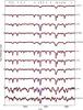 |
Fig. 3 Example of the observed and synthetic spectra around the Ba ii line at 585.36 nm. The solid blue line corresponds to [Ba/Fe] = 0. |
5.2. s-process abundances
Atomic lines were carefully selected over the whole HERMES spectral range using both synthetic and observed spectra. They are listed in Table A.1. Whenever possible, we tried to select lines for each species from both neutral and singly ionized states (excluding strong resonance lines of neutral species known to suffer from NLTE effects).
The only observable lines of Sr ii are the strong lines below 430.5 nm, which are too strongly blended to derive reliable abundances. We therefore only used Sr i lines. Of the eight selected Sr i lines, the line at 687.83 nm is often blended by telluric O2, the resonance line at 460.73 nm is known to suffer from NLTE effects and to give abundances lower than that from higher excitation lines. The line at 707.01 nm has been used in all the target stars except for 14 Aur C and V1261 Aur. In 14 Aur C, the two lines at 640.85 and 707.01 nm are not observable because they blend with other lines as a result of rapid rotation or are lost in the noise. Instead, the strong Sr ii line around 416 nm seems to provide a reliable estimate of the Sr abundance. In V1261 Ori, the two Sr i lines at 640.85 and 707.01 nm are too blended, and we used instead two Sr i lines at 687.83 and 689.26 nm, even though the continuum placement remains the largest uncertainty.
For Y, we mainly used clean lines of Y ii that are more numerous than Y i lines. The cleanest and most useful Y ii lines in our sample are located at 528.98, 540.28, 572.89, and 679.54 nm. The other lines used are listed in Appendix A.
For Zr, we mainly used lines of Zr i, since they are more numerous than Zr ii lines. Lines of Zr i between 800 and 850 nm, when useful, give abundances systematically stronger by about ~0.5 dex. For 14 Aur C, only Zr ii lines below 540 nm can be used for the abundance determination. Since V1261 Ori is veiled by ZrO molecular bands, we used the same lines (between 740 and 758 nm) as those used by Smith & Lambert (1990) to derive the Zr abundance. Lines above 800 nm are useable but give somewhat higher abundances, as already mentioned.
For s-process elements belonging to the second peak (Ba, La, and Ce), only neutral lines are available for Ba. We did not use the Ba ii resonance lines at 455.4 and 493.4 nm in the abundance analysis because of the known NLTE effects (see e.g. Olshevsky & Shchukina 2007), except in 14 Aur C, where too few other lines are available. We mainly used the Ba ii lines at 585.37, 614.17, and 649.69 nm and the Ba i line at 748.81 nm.
Many lines (about 30) are available for La and Ce in the HERMES wavelength range. The most useful La ii lines are located at 529.08, 530.20, 530.35, 617.27, 639.05, and 677.43 nm. The most useful Ce ii lines are located at 456.24, 533.06, 604.34, 802.56, 871.67, and 877.21 nm. The Ce ii lines are the strongest in V1261 Ori, which indeed has the largest Ce overabundance ([Ce/Fe] = 1.29 dex) in our sample.
To illustrate the good agreement between observed and synthetic spectra, we show in Fig. 3 the spectral region around the Ba ii 585.36 nm line, which is well visible in the entire sample. The synthetic spectra in blue are computed with [Ba/Fe] = 0, whereas the red ones are computed with the appropriate [Ba/Fe] abundances as listed in Table 5. The red synthetic spectra nicely reproduce the observed spectra, especially for the fast rotators V1379 Aql and 14 Aur C. The fit is slightly worse for the cooler S stars V1261 Ori and IT Vir because of the presence of numerous molecular lines, but it is nevertheless possible to derive the Ba abundance reliably.
5.3. Uncertainties on s-process abundances
We investigated the effect on the s-process abundances of the uncertainties from the atmospheric parameters, adopting as typical uncertainties on these parameters (Table 2) the values σTeff=± 50 K, σlog g = ± 0.3 dex, σ[Fe/H]=± 0.10 dex, and σξ = ± 0.10 km s-1.
The statistical uncertainty σstat listed in Table 6 is the line-to-line dispersion divided by  , where N is the number of lines used for a given element (Table 6). This statistical uncertainty takes not only uncertainties on atomic data into account, but also those on continuum location and line-profile mismatch problems.
Statistical (σstat) and model-induced (i.e. σTeff, σlog g, σ[Fe/H], and σξ) uncertainties were quadratically added (thus assuming independence between them, as is common practice, although in reality they may be correlated, as discussed by Johnson 2002) to obtain the total uncertainty σtot for each s-process element (which may thus be overestimated). We performed this analysis on ζ Cyg as it is representative of the whole sample (see Fig. 4). The estimated uncertainties are given in Table 6. We note that the uncertainties on the absolute s-process abundances given in Table 4 are only the line-by-line dispersion.
Uncertainties on the derived abundances in ζ Cyg.
To derive the uncertainties on the various [X/Fe] abundances (as listed in Table 5), we added the uncertainties on the absolute abundances A(Fe) and A(X) quadratically. The resulting uncertainties are expressed as  (1)where σ⊙(X) denotes the uncertainty on the solar abundance of species X as given by Grevesse et al. (2007). The corresponding σX uncertainties are listed in Table 5 and plotted in Figs. 4 and 5.
5.4. Comparison with previous studies
V1261 Ori (HD 35155). This star has been analysed by Smith & Lambert (1990), who found the second-peak s-process elements (Ba, La, Ce, Nd) to be enriched by more than 1 dex, as we do. However, Smith & Lambert (1990) found no overabundance in excess of 0.23 dex for Y and Zr, whereas we find these elements to be overabundant by more than 1 dex. We stress that both the models and the line data are very different between the two studies.
IT Vir. Smith (1984) derived the CNO abundances in IT Vir, but did not confirm the large N abundance that we obtain for that star ([N/Fe] = 1.1 to 1.4 dex – Table 3 –, as compared to 0.52 dex for Smith 1984). This large N overabundance is accompanied with a low 12C/13C ratio of 8 (Smith 1984), which could hint at CN processing. However, similarly low 12C/13C ratios are a common feature among barium stars (Smith 1984; Barbuy et al. 1992), without being associated with N overabundances as large as the one we found for IT Vir. We found that regardless of the effective temperature or gravity adopted for this star (Teff = 3900 or 4200 K, log g = 0 or 1 dex; see Sect. 4), the large [N/Fe] overabundance remains. Even after carefully rederiving O and C abundances, [N/Fe] is still larger than 1 dex. Formerly, the largest N abundances observed in barium stars were [N/Fe] = 0.7 dex in HD 27271 and 0.65 dex in HD 60197 (Barbuy et al. 1992). It may be relevant here to note that IT Vir has one of the largest Roche-lobe filling factors of barium stars, since it has a moderately short orbital period (186 d), but a comparatively large radius (~55 R⊙; Jorissen et al. 1995). As a consequence, Jorissen and collaborators reported ellipsoidal variations for this star. The associated faster rotation, tidal deformations, and departure from spherical symmetry will trigger meridional currents and deep mixing, and the observed large N abundance in IT Vir could perhaps be related to such processes currently occurring in the red giant (see for instance Decressin et al. 2009, for a discussion of rotation-induced mixing and the resulting surface enhancement in nitrogen).
The s-process abundances agree well for Sr, Y, and Ce, but Zr, Ba, and La are found to be more abundant by about 1 dex in our study than the values reported by Smith (1984).
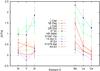 |
Fig. 4 First-peak (Sr, Y, Zr) and second-peak (Ba, La, Ce) s-process abundances relative to Fe. |
56 Peg. It is the first time that an s-process abundance analysis is performed for 56 Peg, and it confirms its barium nature. Because of the high luminosity of 56 Peg (it is classified as K0Iab – confirmed by the low gravity of log g = 1.3; Table 2), the increased strength of the Ba ii lines, which led to its classification as a barium star, might have been caused by the low atmospheric pressure, a consequence of Saha equation. But our abundance analysis reveals a weak albeit clear s-process enhancement.
ζ Cap and ζ Cyg. These stars were analysed by Smiljanic et al. (2007). The agreement between the two studies on the s-process abundances is reasonable (in particular, both studies find large overabundances in ζ Cap and much milder ones in ζ Cyg), except for Sr in ζ Cap: Smiljanic et al. (2007) obtained [Sr/Fe] = 2.21, as compared to 1.02 in the present study. Smiljanic et al. (2007) used the single Sr i resonance line at 460.73 nm, whereas we used that line and a line at 707.01 nm. Based solely on the 460.73 nm line, we find [Sr/Fe] = 0.99, and this value agrees well with the value 1.07 based on the 707.01 nm line. The reason for the discrepancy between the Sr abundances derived from the Sr i resonance line at 460.73 nm here and in Smiljanic et al. (2007) must partly reside in the different log gf values used [0.069 by Smiljanic et al. (2007) against 0.283 in our work, from NIST with the AA accuracy – see Appendix A], and partly in the different atmospheric parameters adopted.
DR Dra. Berdyugina (1994), Zacs et al. (1997), and Barisevičius et al. (2010) concluded, like we do, that DR Dra does not exhibit any s-process overabundance.
IP Eri. This star has been analysed by Merle et al. (2014). We rederived the s-process abundances with the same pipeline and methodology, but with a refined line selection for each element. The rederived s-process abundances agree with our previous work within the error bars, and we here obtain lower statistical uncertainties.
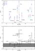 |
Fig. 5 Upper panel: first- (Sr, Y, Zr) and second-peak (Ba, La, Ce) s-process abundances relative to Fe as a function of the WD mass. Lower panel: same as upper panel, but with mean s-process abundances relative to Fe. To guide the eye, the grey zone shows the ±0.25 dex zone without significant enhancement in s-process abundances. |
6. Discussion
The s-process abundance distribution is presented in Fig. 4, which clearly shows that our sample contains both normal stars and stars enriched in s-process elements (and the latter also exhibit enhanced carbon and sometimes nitrogen overabundances; Fig. 6). The origin of the difference between these two stellar categories is clearly revealed when plotting the average s-process abundance, as listed in the last column of Table 5, as a function of the mass of the WD companion (Fig. 5). The expected trend is indeed obtained: s-process overabundances are found in binary stars with a companion WD mass higher than about 0.5 M⊙, that is, the progenitor of the WD went through the thermally pulsing AGB (TP-AGB) phase, was able to synthesize s-process elements in the intershell zone, and these were subsequently dredged up to the surface. Indeed, Hurley et al. (2000) (their Eq. (66)) predicted the minimum CO core mass at the base of the AGB (just at the end of core He-burning) to be at least 0.51 M⊙ (for a star of initial mass 0.9 M⊙). Conversely, when the WD mass is lower than 0.51 M⊙, the s-process synthesis did not occur (because the progenitor did not reach the TP-AGB): s-process overabundances are not observed. There are two marginal cases, namely DR Dra and 14 Aur C, whose WD mass qualifies them for being polluted by s-process material, but which are not. For 14 Aur C, apart from the difficulty imprinted on the analysis by the rapid stellar rotation, the cause for the absence of s-process enrichment could be its unusually short period of three days, which is likely the result of a common-envelope evolution (Han et al. 1995). It is believed that this channel does not lead to substantial accretion during the common-envelope process (Ricker & Taam 2008)2. Nevertheless, the recent occurrence of binary interaction is revealed by the rapid rotation of the star. The same holds true for DR Dra, whose absence of s-process overabundance is slightly more puzzling, however. The long period of DR Dra (904 d) suggests that the rapid rotation responsible for the chromospheric activity be due to spin accretion (Theuns et al. 1996) rather than to tidal coupling, which requires a closer system (Fekel et al. 1993). Thus there has been some binary interaction in the recent past of DR Dra. The absence of s-process overabundance in this star suggests that with a mass estimated at 0.55 M⊙ (Fekel & Simon 1985), either the WD does not originate from a TP-AGB star (Hurley et al. 2000), there was no dredge-up in the TP-AGB star, or there was simply no s-process nucleosynthesis operating.
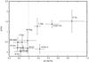 |
Fig. 6 Correlation between the s-process abundances and the carbon + nitrogen abundances. |
The level of s-process overabundances of barium stars varies greatly, from the marginal level of HR 5692, ζ Cyg, and 56 Peg, to the highest level of IT Vir. Two co-existing causes for these variations are readily identified in the literature: on the one hand, the efficiency of the s-process nucleosynthesis in AGB stars varies with metallicity (Clayton 1988; Käppeler et al. 2011), and on the other hand, the efficiency of mass accretion varies with orbital separation (Jorissen & Boffin 1992; Han et al. 1995; Pols et al. 2003). Thus, orbital separation and metallicity could directly control the level of s-process overabundances in barium stars. But all previous studies have concluded that if it exists at all, the correlation between orbital periods and s-process overabundances is weak, and the present study is no exception. For instance, 56 Peg has one of the shortest orbital periods3 of all barium stars (111 d; Griffin 2006), and yet its s-process overabundance level is very moderate. A search for additional parameters (besides metallicity) that might blur the relationship between orbital periods and s-process pollution levels is therefore of interest. Here we suggest that the WD mass, tracing the maximum luminosity reached on the AGB (through the core-mass – luminosity relationship; Herwig et al. 1998), could also play a role in this respect. Indeed, the AGB luminosity is a proxy for the number of thermal pulses experienced by the AGB star (although the initial AGB mass must play a role as well), which in turn governs the s-process level attained in its atmosphere. However, too few stars are available at present to be able to draw any firm conclusion, apart from the observation that large s-process overabundance levels are found at both ends of the CO WD mass range: around 0.6 M⊙ (IT Vir, V1261 Ori) and around 1 M⊙ (ζ Cap).
7. Conclusion
We have analysed a sample of 11 binary systems comprising WD of known masses. High-resolution and high signal-to-noise spectra were collected from the HERMES spectrograph installed at the Mercator 1.2 m telescope. The atmospheric parameters and the CNO and s-process abundances were derived using LTE models. We derived for the first time atmospheric parameters for 14 Aur C (HD 33959C) and s-process element abundances for 56 Peg (HR 8796). The sample includes two S stars that were analysed with new dedicated S-star MARCS model atmospheres. One of them, IT Vir (HD 121447), has the largest overabundance of s-process elements in the sample and has been identified as highly N-enriched. Such a high level of N overabundance could perhaps be related to the photometric variations exhibited by this star and is attributed to ellipsoidal variations as the red giant has a large Roche-filling factor. The ensuing faster rotation could trigger deep mixing, which is known to bring nitrogen to the surface.
Finally, from our homogeneous study of s-process abundances in the primary components of binary systems involving a WD companion, we find that there is a clear relationship between s-process enrichment and WD mass: as expected, primary components in binary systems involving He WDs (thus with a mass lower than about 0.5 M⊙) never show s-process overabundances, as the WD progenitor never reached the TP-AGB.
The low-metallicity carbon dwarf HE 0024-2523, with its 3.4 d orbital period and its strong Pb overabundance, is a noticeable counter-example of this statement, however (Lucatello et al. 2003).
Acknowledgments
This research has been funded by the Belgian Science Policy Office under contract BR/143/A2/STARLAB. T.M. is supported by the FNRS-F.R.S. as temporary post-doctoral researcher under grant No. 2.4513.11. This work was supported by the Fonds de la Recherche Scientifique FNRS under Grant n° T.0198.13. The Mercator telescope is operated thanks to grant number G.0C31.13 of the FWO under the “Big Science” initiative of the Flemish governement. Based on observations obtained with the HERMES spectrograph, supported by the Fund for Scientific Research of Flanders (FWO), the Research Council of K.U.Leuven, the Fonds National de la Recherche Scientifique (F.R.S.-FNRS), Belgium, the Royal Observatory of Belgium, the Observatoire de Genève, Switzerland and the Thüringer Landessternwarte Tautenburg, Germany. This work has made use of the VALD database, operated at Uppsala University, the Institute of Astronomy RAS in Moscow, and the University of Vienna.
References
- Abia, C., & Wallerstein, G. 1998, MNRAS, 293, 89 [NASA ADS] [CrossRef] [Google Scholar]
- Ake, T. B. 1979, ApJ, 234, 538 [NASA ADS] [CrossRef] [Google Scholar]
- Ake, III, T. B., Johnson, H. R., & Ameen, M. M. 1991, ApJ, 383, 842 [NASA ADS] [CrossRef] [Google Scholar]
- Alvarez, R., & Plez, B. 1998, A&A, 330, 1109 [NASA ADS] [Google Scholar]
- Asplund, M. 2005, ARA&A, 43, 481 [NASA ADS] [CrossRef] [Google Scholar]
- Böhm-Vitense, E., Carpenter, K., Robinson, R., Ake, T., & Brown, J. 2000, ApJ, 533, 969 [NASA ADS] [CrossRef] [Google Scholar]
- Barbuy, B., Jorissen, A., Rossi, S. C. F., & Arnould, M. 1992, A&A, 262, 216 [NASA ADS] [Google Scholar]
- Barisevičius, G., Tautvaišienė, G., Berdyugina, S., Chorniy, Y., & Ilyin, I. 2010, Balt. Astron., 19, 157 [NASA ADS] [Google Scholar]
- Berdyugina, S. V. 1994, Astron. Lett., 20, 796 [NASA ADS] [Google Scholar]
- Bessell, M. S., Castelli, F., & Plez, B. 1998, A&A, 333, 231 [NASA ADS] [Google Scholar]
- Bidelman, W. P., & Keenan, P. C. 1951, ApJ, 114, 473 [NASA ADS] [CrossRef] [Google Scholar]
- Bilíková, J., Chu, Y.-H., Gruendl, R. A., & Maddox, L. A. 2010, AJ, 140, 1433 [NASA ADS] [CrossRef] [Google Scholar]
- Böhm-Vitense, E. 1980, ApJ, 239, L79 [NASA ADS] [CrossRef] [Google Scholar]
- Böhm-Vitense, E., Nemec, J., & Proffitt, C. 1984, ApJ, 278, 726 [NASA ADS] [CrossRef] [Google Scholar]
- Burleigh, M. R., Barstow, M. A., & Fleming, T. A. 1997, MNRAS, 287, 381 [NASA ADS] [CrossRef] [Google Scholar]
- Burleigh, M. R., Barstow, M. A., & Holberg, J. B. 1998, MNRAS, 300, 511 [NASA ADS] [CrossRef] [Google Scholar]
- Christian, D. J., Vennes, S., Thorstensen, J. R., & Mathioudakis, M. 1996, AJ, 112, 258 [NASA ADS] [CrossRef] [Google Scholar]
- Clayton, D. D. 1988, MNRAS, 234, 1 [NASA ADS] [CrossRef] [Google Scholar]
- Decressin, T., Charbonnel, C., Siess, L., et al. 2009, A&A, 505, 727 [NASA ADS] [CrossRef] [EDP Sciences] [Google Scholar]
- Den Hartog, E. A., Lawler, J. E., & Wood, M. P. 2014a, ApJS, 215, 7 [NASA ADS] [CrossRef] [Google Scholar]
- Den Hartog, E. A., Ruffoni, M. P., Lawler, J. E., et al. 2014b, ApJS, 215, 23 [NASA ADS] [CrossRef] [Google Scholar]
- Dominy, J. F., & Lambert, D. L. 1983, ApJ, 270, 180 [NASA ADS] [CrossRef] [Google Scholar]
- Fekel, F. X., & Simon, T. 1985, AJ, 90, 812 [NASA ADS] [CrossRef] [Google Scholar]
- Fekel, F. C., Henry, G. W., Busby, M. R., & Eitter, J. J. 1993, AJ, 106, 2370 [NASA ADS] [CrossRef] [Google Scholar]
- Frankowski, A., & Jorissen, A. 2006, The Observatory, 126, 25 [NASA ADS] [Google Scholar]
- Gray, R. O., Corbally, C. J., Garrison, R. F., McFadden, M. T., & Robinson, P. E. 2003, AJ, 126, 2048 [NASA ADS] [CrossRef] [Google Scholar]
- Gray, R. O., McGahee, C. E., Griffin, R. E. M., & Corbally, C. J. 2011, AJ, 141, 160 [NASA ADS] [CrossRef] [Google Scholar]
- Grevesse, N., Asplund, M., & Sauval, A. J. 2007, Space Sci. Rev., 130, 105 [Google Scholar]
- Griffin, R. F. 2006, The Observatory, 126, 1 [NASA ADS] [Google Scholar]
- Griffin, R. F., & Keenan, P. C. 1992, The Observatory, 112, 168 [Google Scholar]
- Gustafsson, B., Edvardsson, B., Eriksson, K., et al. 2008, A&A, 486, 951 [NASA ADS] [CrossRef] [EDP Sciences] [Google Scholar]
- Han, Z., Eggleton, P. P., Podsiadlowski, P., & Tout, C. A. 1995, MNRAS, 277, 1443 [NASA ADS] [CrossRef] [Google Scholar]
- Herwig, F., Schoenberner, D., & Bloecker, T. 1998, A&A, 340, L43 [NASA ADS] [Google Scholar]
- Hoard, D. W., Wachter, S., Sturch, L. K., et al. 2007, AJ, 134, 26 [NASA ADS] [CrossRef] [Google Scholar]
- Holweger, H. 1979, in Liege International Astrophysical Colloquia 22, eds. A. Boury, N. Grevesse, & L. Remy-Battiau, 117 [Google Scholar]
- Hurley, J. R., Pols, O. R., & Tout, C. A. 2000, MNRAS, 315, 543 [NASA ADS] [CrossRef] [Google Scholar]
- Jeffries, R. D., & Smalley, B. 1996, A&A, 315, L19 [NASA ADS] [Google Scholar]
- Jofre, P., Heiter, U., Soubiran, C., et al. 2014, A&A, 564, A133 [NASA ADS] [CrossRef] [EDP Sciences] [Google Scholar]
- Johnson, J. A. 2002, ApJS, 139, 219 [NASA ADS] [CrossRef] [Google Scholar]
- Jorissen, A., & Boffin, H. M. J. 1992, in Binaries as Tracers of Stellar Formation, eds. A. Duquennoy, & M. Mayor (Cambridge: Cambridge University Press), 110 [Google Scholar]
- Jorissen, A., Mayor, M., Manfroid, J., & Sterken, C. 1992, Information Bulletin on Variable Stars, 3730, 1 [NASA ADS] [Google Scholar]
- Jorissen, A., Hennen, O., Mayor, M., Bruch, A., & Sterken, C. 1995, A&A, 301, 707 [NASA ADS] [Google Scholar]
- Jorissen, A., Schmitt, J. H. M. M., Carquillat, J. M., Ginestet, N., & Bickert, K. F. 1996, A&A, 306, 467 [NASA ADS] [Google Scholar]
- Jorissen, A., Van Eck, S., Mayor, M., & Udry, S. 1998, A&A, 332, 877 [NASA ADS] [Google Scholar]
- Käppeler, F., Gallino, R., Bisterzo, S., & Aoki, W. 2011, Rev. Mod. Phys., 83, 157 [NASA ADS] [CrossRef] [EDP Sciences] [Google Scholar]
- Kovacs, N. 1983, A&A, 120, 21 [NASA ADS] [Google Scholar]
- Kupka, F., Dubernet, M.-L., & VAMDC Collaboration. 2011, Balt. Astron., 20, 503 [Google Scholar]
- Landsman, W., Simon, T., & Bergeron, P. 1993, PASP, 105, 841 [NASA ADS] [CrossRef] [Google Scholar]
- Lucatello, S., Gratton, R., Cohen, J. G., et al. 2003, AJ, 125, 875 [NASA ADS] [CrossRef] [Google Scholar]
- Masseron, T. 2006, Ph.D. Thesis, Observatoire de Paris, France [Google Scholar]
- Masseron, T., Plez, B., Van Eck, S., et al. 2014, A&A, 571, A47 [NASA ADS] [CrossRef] [EDP Sciences] [Google Scholar]
- McClure, R. D., & Woodsworth, A. W. 1990, ApJ, 352, 709 [NASA ADS] [CrossRef] [Google Scholar]
- McClure, R. D., Fletcher, J. M., & Nemec, J. M. 1980, ApJ, 238, L35 [NASA ADS] [CrossRef] [Google Scholar]
- Merle, T., Jorissen, A., Masseron, T., et al. 2014, A&A, 567, A30 [NASA ADS] [CrossRef] [EDP Sciences] [Google Scholar]
- Neyskens, P., van Eck, S., Jorissen, A., et al. 2015, Nature, 517, 174 [NASA ADS] [CrossRef] [PubMed] [Google Scholar]
- Olshevsky, V. L., & Shchukina, N. G. 2007, in Modern solar facilities – advanced solar science, eds. F. Kneer, K. G. Puschmann, & A. D. Wittmann (Göttingen: Universitäts Verlag), 307 [Google Scholar]
- Plez, B. 2012, Astrophysics Source Code Library, 5004 [Google Scholar]
- Pols, O. R., Karakas, A. I., Lattanzio, J. C., & Tout, C. A. 2003, in Symbiotic Stars Probing Stellar Evolution, eds. R. L. M. Corradi, J. Mikolajewska, & T. J. Mahoney, ASP Conf. Ser., 303, 290 [Google Scholar]
- Prugniel, P., Vauglin, I., & Koleva, M. 2011, A&A, 531, A165 [NASA ADS] [CrossRef] [EDP Sciences] [Google Scholar]
- Raskin, G., van Winckel, H., Hensberge, H., et al. 2011, A&A, 526, A69 [NASA ADS] [CrossRef] [EDP Sciences] [Google Scholar]
- Ricker, P. M., & Taam, R. E. 2008, ApJ, 672, L41 [NASA ADS] [CrossRef] [Google Scholar]
- Ruffoni, M. P., Den Hartog, E. A., Lawler, J. E., et al. 2014, MNRAS, 441, 3127 [NASA ADS] [CrossRef] [Google Scholar]
- Schindler, M., Stencel, R. E., Linsky, J. L., Basri, G. S., & Helfand, D. J. 1982, ApJ, 263, 269 [Google Scholar]
- Siess, L., Davis, P. J., & Jorissen, A. 2014, A&A, 565, A57 [NASA ADS] [CrossRef] [EDP Sciences] [Google Scholar]
- Smiljanic, R., Porto de Mello, G. F., & da Silva, L. 2007, A&A, 468, 679 [NASA ADS] [CrossRef] [EDP Sciences] [Google Scholar]
- Smith, V. V. 1984, A&A, 132, 326 [NASA ADS] [Google Scholar]
- Smith, V. V., & Lambert, D. L. 1990, ApJS, 72, 387 [NASA ADS] [CrossRef] [Google Scholar]
- Sneden, C., Lucatello, S., Ram, R. S., Brooke, J. S. A., & Bernath, P. 2014, ApJS, 214, 26 [Google Scholar]
- Stefanik, R. P., Torres, G., Latham, D. W., et al. 2011, AJ, 141, 144 [NASA ADS] [CrossRef] [Google Scholar]
- Theuns, T., Boffin, H. M. J., & Jorissen, A. 1996, MNRAS, 280, 1264 [NASA ADS] [CrossRef] [Google Scholar]
- Van Eck, S., Neyskens, P., Plez, B., et al. 2011, J. Phys. Conf. Ser., 328, 012009 [NASA ADS] [CrossRef] [Google Scholar]
- van Leeuwen, F. 2007, A&A, 474, 653 [NASA ADS] [CrossRef] [EDP Sciences] [Google Scholar]
- Vennes, S., Mathioudakis, M., Doyle, J. G., Thorstensen, J. R., & Byrne, P. B. 1995, A&A, 299, L29 [NASA ADS] [Google Scholar]
- Vennes, S., Christian, D. J., Mathioudakis, M., & Doyle, J. G. 1997, A&A, 318, L9 [NASA ADS] [Google Scholar]
- Vennes, S., Christian, D. J., & Thorstensen, J. R. 1998, ApJ, 502, 763 [NASA ADS] [CrossRef] [Google Scholar]
- Zacs, L., Musaev, F. A., Bikmaev, I. F., & Alksnis, O. 1997, A&AS, 122, 31 [NASA ADS] [CrossRef] [EDP Sciences] [Google Scholar]
Appendix A: Atomic linelist
Atomic line list.
Appendix B: Molecular line list
Molecular line list.
All Tables
Absolute s-process element abundances A(X) (defined as A(X) = log [n(X) /n(H)] + 12, where n(X) and n(H) are the number densities of X and H).
All Figures
|
Fig. 1 Ca II H and K lines for the sample stars. For comparison, the spectra of the Sun and Arcturus are plotted at the bottom and top of the figure, respectively. Evidence of activity is present in 63 Eri, IP Eri, V1379 Aql, DR Dra, and 56 Peg. |
| In the text | |
|
Fig. 2 Surface gravity vs. effective temperature for the sample stars. |
| In the text | |
|
Fig. 3 Example of the observed and synthetic spectra around the Ba ii line at 585.36 nm. The solid blue line corresponds to [Ba/Fe] = 0. |
| In the text | |
|
Fig. 4 First-peak (Sr, Y, Zr) and second-peak (Ba, La, Ce) s-process abundances relative to Fe. |
| In the text | |
|
Fig. 5 Upper panel: first- (Sr, Y, Zr) and second-peak (Ba, La, Ce) s-process abundances relative to Fe as a function of the WD mass. Lower panel: same as upper panel, but with mean s-process abundances relative to Fe. To guide the eye, the grey zone shows the ±0.25 dex zone without significant enhancement in s-process abundances. |
| In the text | |
|
Fig. 6 Correlation between the s-process abundances and the carbon + nitrogen abundances. |
| In the text | |
Current usage metrics show cumulative count of Article Views (full-text article views including HTML views, PDF and ePub downloads, according to the available data) and Abstracts Views on Vision4Press platform.
Data correspond to usage on the plateform after 2015. The current usage metrics is available 48-96 hours after online publication and is updated daily on week days.
Initial download of the metrics may take a while.