| Issue |
A&A
Volume 585, January 2016
|
|
|---|---|---|
| Article Number | A102 | |
| Number of page(s) | 8 | |
| Section | Stellar atmospheres | |
| DOI | https://doi.org/10.1051/0004-6361/201527491 | |
| Published online | 23 December 2015 | |
Research Note
Non-LTE analysis of copper abundances for the two distinct halo populations in the solar neighborhood⋆
1
Key Laboratory of Optical Astronomy, National Astronomical Observatories,
Chinese Academy of Sciences,
20A Datun Road, Chaoyang District,
100012
Beijing,
PR China
e-mail:
This email address is being protected from spambots. You need JavaScript enabled to view it.
2
University of Chinese Academy of Sciences,
No.19A Yuquan Road, 100049,
Beijing, PR
China
3
Stellar Astrophysics Centre, Department of Physics and Astronomy,
Aarhus University, 8000
Aarhus C,
Denmark
e-mail:
This email address is being protected from spambots. You need JavaScript enabled to view it.
Received: 1 October 2015
Accepted: 23 October 2015
Abstract
Context. Two distinct halo populations were found in the solar neighborhood by a series of works. They can be clearly separated by [α/Fe] and several other elemental abundance ratios including [Cu/Fe]. Very recently, a non-local thermodynamic equilibrium (non-LTE) study revealed that relatively large departures exist between LTE and non-LTE results in copper abundance analysis. The study also showed that non-LTE effects of neutral copper vary with stellar parameters and thus affect the [Cu/Fe] trend.
Aims. We aim to derive the copper abundances for the stars from the sample of Nissen & Schuster (2010) with both LTE and non-LTE calculations. Based on our results, we study the non-LTE effects of copper and investigate whether the high-α population can still be distinguished from the low-α population in the non-LTE [Cu/Fe] results.
Methods. Our differential abundance ratios are derived from the high-resolution spectra collected from VLT/UVES and NOT/FIES spectrographs. Applying the MAFAGS opacity sampling atmospheric models and spectrum synthesis method, we derive the non-LTE copper abundances based on the new atomic model with current atomic data obtained from both laboratory and theoretical calculations.
Results. The copper abundances determined from non-LTE calculations are increased by 0.01 to 0.2 dex depending on the stellar parameters compared with the LTE results. The non-LTE [Cu/Fe] trend is much flatter than the LTE one in the metallicity range −1.6 < [ Fe / H ] < −0.8. Taking non-LTE effects into consideration, the high- and low-α stars still show distinguishable copper abundances, which appear even more clear in a diagram of non-LTE [Cu/Fe] versus [Fe/H].
Conclusions. The non-LTE effects are strong for copper, especially in metal-poor stars. Our results confirmed that there are two distinct halo populations in the solar neighborhood. The dichotomy in copper abundance is a peculiar feature of each population, suggesting that they formed in different environments and evolved obeying diverse scenarios.
Key words: Galaxy: evolution / Galaxy: halo / line: formation / line: profiles / stars: abundances / stars: atmospheres
Based on observations made with the FIbre fed Echelle Spectrograph (FIES) at the Nordic Optical Telescope (NOT) on La Palma, and on data from the European Southern Observatory ESO/ST-ECF Science Archive Facility (programs 65.L-0507, 67.D-0086, 67.D-0439, 68.D-0094, 68.B-0475, 69.D-0679, 70.D-0474, 71.B-0529, 72.B-0585, 76.B-0133 and 77.B-0507).
© ESO, 2015
1. Introduction
To understand how the Milky Way formed and evolved is one of the key and fundamental questions of modern astrophysics. The stellar populations and the substructures in the Galaxy are the most natural indicators of the processes that the Milky Way experienced. Much effort has been invested into revealing the composition of the stellar populations in the Galactic halo. The classic work of Eggen et al. (1962) implies that the stars in the Galactic halo belong to one population, which originated from the material that accumulated during the collapse of the protogalaxy. This single-component halo was considered to be plausible for a long time, yet different scenarios were raised in the following decades. Searle & Zinn (1978) found clues from globular clusters indicating that there are two halo populations that can be divided according to their horizontal branch morphology. Since then, evidence from different works continued to challenge the single-component halo model (e.g., Zinn 1993; Carney et al. 1996; Wilhelm et al. 1996; Kinman et al. 2007; Lee et al. 2007; Miceli et al. 2008). Recent data from large survey programs also prefer a more complex Galactic halo that consists of at least two populations (Carollo et al. 2007; Jofré & Weiss 2011; Hawkins et al. 2015).
The variation of relative abundances as a function of stellar [Fe/H] is a powerful tool for identifying different populations because various species of elements may have been synthesized on different timescales and in various environments (Tinsley 1979). The α-elements (e.g., Mg, Si, Ca, and Ti) are very important. In contrast to iron, which is mainly synthesized in type Ia supernovae (SNe Ia) on a relatively long timescale, the dominate source of α-elements is the shorter-lived type II supernovae (SNe II), therefore the [α/Fe] can represent an ideal cosmos-clock to trace the history of chemical evolution. If the halo is composed of more than one component, it would be reasonable to expect that systematic differences in the stellar properties also exist for the halo stars in the solar neighborhood, where the α-element abundances can be measured precisely based on high-resolution spectra. Previous studies have found variations in [α/Fe] between the inner- and outer-halo stars, but it is unclear whether there is a dichotomy in the [α/Fe] pattern or not (see discussion in Nissen & Schuster 2011). In a series of works, Nissen & Schuster (2010, 2011; hereafter cited as NS10 and NS11, respectively), Schuster et al. (2012) and Nissen & Schuster (2012) detected two distinct halo populations with dual [α/Fe] distributions in the solar neighborhood. The two populations also show differences in other properties, including [Cu/Fe]. NS11 found that the high-α stars have a tight [Cu/Fe] trend that is similar to that of the thick-disk population, while the low-α stars have a much looser [Cu/Fe] trend and a systematic [Cu/Fe] deficiency compared to the high-α stars, presenting a clear distinction in the [Cu/Fe] versus [Fe/H] diagram.
However, the abundance analysis in NS11 was based on LTE assumption. Previous works on non-LTE effects have demonstrated the importance of its effect, especially for metal-poor stars (e.g., Zhao & Gehren 2000; Gehren et al. 2004; Bergemann & Gehren 2008; Shi et al. 2009). Copper is thought to be one of the elements that may suffer strong non-LTE effects. Several studies have reported that the abundances derived from some of the Cu i or Cu ii lines are inconsistent with each other (Bihain et al. 2004; Bonifacio et al. 2010; Roederer et al. 2012, 2014). Very recently, Yan et al. (2015) proposed a non-LTE analysis for the copper abundance in late-type metal-poor stars, showing that the value of [Cu/Fe] can be underestimated by up to 0.2 dex in LTE analysis. The underestimation is correlated with stellar parameters, especially with the metallicity. It is therefore interesting to investigate whether the separation in [Cu/Fe] reported in NS11 still exists when non-LTE effects are taken into consideration.
To derive a reliable [Cu/Fe] trend and reveal the non-LTE effect on distinguishing different populations, we reanalyzed the copper abundances for the sample stars that were used in NS10 and NS11. The results are given with both LTE and non-LTE calculations. In Sect. 2 we describe how we obtained the LTE and non-LTE copper abundances, including the details of non-LTE calculations. Section 3 describes the results and error analysis. The conclusions are presented in Sect. 4.
2. Methods
2.1. Non-LTE calculations
We have presented the details of copper atomic model in our previous work (Shi et al. 2014). In general, our final atomic model consists of 96 energy levels of Cu i plus the ground state of Cu ii. Laboratory data from NIST1 and Sugar & Musgrove (1990) were used for the 51 levels with low-excitation energy, while for the rest of the levels with higher excitation energy, we applied the theoretical work of Liu et al. (2014), which is based on the R-matrix approach (Burke et al. 1971; Liu et al. 2011). Fine structures were considered to the level of  . Probabilities for all the 1089 bound-bound transitions applied for Cu i and the photoionization cross-sections were also calculated by Liu et al. (2014). In addition, the excitation and ionization caused by inelastic collisions with electrons and hydrogen atoms were taken into account based on a series of theoretical works (see details in Shi et al. 2014). We scaled the collisional rates with neutral hydrogen by a factor of SH = 0.1 to avoid the overestimation (Barklem et al. 2011) from the Drawin fomula (Drawin 1968, 1969) following Shi et al. (2014). A revised version of the DETAIL program (Butler & Giddings 1985) with accelerated lambda iteration was employed to carry out the calculations.
Figure 1 shows the calculated departure coefficients (bi) of the selected levels as a function of the continuum optical depth at 5000 Å (log τ5000) for the model atmosphere of G05-40, which has a temperature and metallicity representative of the sample stars. Here bi represents the ratio between the number densities given by non-LTE calculations ( ) and LTE (
 ) calculations. The departure coefficients for the most important levels of Cu i and the ground state of Cu ii are shown in the figure. The overionization becomes significant outside the layers with log τ5000≃ 0.5, depopulating the lower energy levels such as
  and
and  , and thus leading to an underestimation of the copper abundance from the LTE analysis.
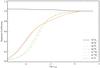 |
Fig. 1 Departure coefficients bi of the selected energy levels (listed in the figure) as a function of continuum optical depth at 5000 Å for the model atmosphere of G05-40. The collision with neutral hydrogen was scaled by a factor of 0.1 following Shi et al. (2014). |
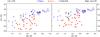 |
Fig. 2 Abundance ratios [Cu/Fe] as a function of [Fe/H] for the program stars, where LTE and non-LTE results are represented in the left and right panel, respectively. The high-α (open blue circles), low-α (filled red circles) and thick-disk populations (black crosses) are indicated (see the online version for color copies of the figures). G112-42 and G112-43 are connected with a straight line. |
2.2. Copper abundance analysis
We investigated 94 dwarfs with effective temperatures between 5200 K and 6300 K and a metallicity range from −1.6 to −0.4, of which 78 belong to the halo population and the remaining 16 are from the thick disk. The stars were observed using either the ESO/VLT UVES spectrograph (with a resolution R ≃ 55 000 and a signal-to-noise ratio S/N ~ 250−500) or the NOT/FIES spectrograph (R ≃ 40 000, S/N ≃ 140−200). Details about the sample and observations are reported in NS10 and Schuster et al. (2006). In addition, we also directly employed the stellar parameters from NS10.
In our copper abundance analysis, we applied the MAFAGS opacity sampling (OS) model atmosphere developed and updated by Grupp (2004) and Grupp et al. (2009). This is a one-dimensional plane-parallel model that is in hydrostatic equilibrium with chemical homogeneity throughout all the atmospheric layers. The turbulent convection is treated with the improved model presented by Canuto & Mazzitelli (1992). 86 000 frequency points are randomly sampled, including both continuous opacities and line opacities which are calculated based on the line list of Kurucz (2009). The model was also employed in several previous non-LTE works (Mashonkina et al. 2011; Shi et al. 2014; Yan et al. 2015). The differences between MAFAGS and MARCS OS model have been discussed in Shi et al. (2014), and no significant departure was found.
For the fully differential abundance evaluation with respect to the Sun, three lines are employed to perform the spectrum synthesis, which are 5105.5 Å, 5218.2 Å, and 5782.1 Å. The λ5782.1 is not available in the UVES spectra as mentioned in NS11, so it only takes a part in the analysis of the FIES spectra. The oscillator strengths (log gf) used in this work were calibrated with respect to the Sun as described by Shi et al. (2014). The transitions of hyperfine structure (HFS) were computed based on the Russell-Saunders (RS) coupling method, with the input parameters being adopted according to Biehl (1976). The van der Waals damping constants (log C6) for Cu i lines were obtained based on Anstee & O’Mara (1991, 1995). The transitions and the relevant line data are presented in Table 1 of Yan et al. (2015).
We used the Spectrum Investigation Utility (SIU) developed by Reetz (1991) to perform the line formation. In the program, the external broadening mechanisms are combined together as one Gauss profile to be convolved with the synthetic spectrum during the line profile fitting. In addition, the isotope ratio of copper (63Cu and 65Cu) was set to be 0.69:0.31 following Asplund et al. (2009) (see Fig. A.1 for an example of the fitting of the 5105.5 Å line). We adopted log ε⊙(Cu) = 4.25 (Lodders et al. 2009) as the “absolute” solar copper abundance, which is measured from meteorites.
3. Results
Similar to NS11, the copper abundances were derived for 78 stars of the sample. The remaining 16 stars do not have recognizable or clear enough Cu i line profiles in their spectra. We present our detailed results in Tables A.1 and A.2, which include both LTE and non-LTE copper abundances derived from individual lines for each star. The stellar [Cu/Fe] was assigned by computing the arithmetical mean value of all the valid line results for each star, and the error given in the tables is derived from line-to-line scatter. As seen from Tables A.1 and A.2, there is no large line-to-line scatter for the copper abundance (see also Fig. A.2). Figure 2 shows our final stellar [Cu/Fe] obtained from LTE (left panel) and non-LTE calculations (right panel) as a function of [Fe/H]. For a better comparison, the coordinate scales in Fig. 2 are exactly the same in both panels. The high-α, low-α, and thick-disk populations are indicated by different symbols. G112-42 and G112-43 are probably components of a binary system, therefore we connect them with a straight line in the figure the same as NS11.
Our LTE [Cu/Fe] trend (Fig. 2 left panel) agrees quite well with that in NS11. The stars that have higher [α/Fe] tend to have higher [Cu/Fe] compared to the low-α stars in the same metallicity range. The high-α stars also show a tightly increasing [Cu/Fe] trend toward higher metallicity, which overlaps with the thick-disk stars. In contrast, the low-α stars lie below the other two populations in the figure, and they present a much looser relation between [Cu/Fe] and [Fe/H], showing large scatters at a given metallicity. The consistency of the two works is expected because we adopted the same stellar parameters and similar log gf values. Still, the agreement is remarkable (see Fig. A.3) considering that NS11 applied equivalent widths to derive Cu abundances, whereas we used profile fitting.
When considering the non-LTE results (Fig. 2 right panel), it is still tenable that high- and low-α stars can be separated by their [Cu/Fe] values, suggesting they may have different origins and evolution histories, as discussed in NS10 and NS11. This separation is even clearer in the lower metallicity range for non-LTE results, namely from −1.6 to −1.1. The clearer separation is mainly because the non-LTE effects for copper are more sensitive to low metallicity, which significantly reduces the number density of the free electrons in the stellar atmosphere, leading to a lower collisional rate that is not efficient enough for the environment to reach the LTE state.
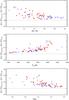 |
Fig. 3 Differences in [Cu/Fe] between non-LTE and LTE as a function of metallicity (top panel), effective temperature (middle panel), and surface gravity (bottom panel). The symbols are the same as in Fig. 2. |
The non-LTE corrections are dominated by the properties of the energy levels and the transitions between them, and consequently, they differ from line to line. In general, the non-LTE effects tend to increase the copper abundances when [Fe/H] < 0 (Tables A.1 and A.2). Yan et al. (2015) found that the LTE analyses underestimated the copper abundances by 0.01 to 0.2 dex depending on the stellar parameters; similar results can be seen in this work. In addition, the departure from LTE changes the [Cu/Fe] trend significantly at the low-metallicity end. A much flatter [Cu/Fe] distribution in the metallicity range −1.6 < [ Fe / H ] < −0.8 is shown in Fig. 2 (compared with the left panel) for thick-disk and halo stars, a linear least-squares fitting gives a slope of 0.54 to LTE results and 0.33 to non-LTE results. The non-LTE departures as functions of stellar [Fe/H], Teff, and log g are shown in Fig. 3 (top, middle, and bottom panel, respectively). The top panel shows an increasing trend toward the lower metallicity, which is also presented by Yan et al. (2015). This dependence affects the [Cu/Fe] values in metal-poor stars much more than that in metal-rich stars and thus flattens the [Cu/Fe] versus [Fe/H] relation. The non-LTE effects tend to be strong for hot stars with two outsiders whose temperatures are the highest in our sample (middle panel). At higher temperature, Cu i starts to become a minority species, thus small corrections from statistical equilibrium to the neutral copper can lead to large abundance deviations, but this is not the case if the temperature continues to increase because the Cu i lines become weak; they form in a much deeper layer of a stellar atmosphere, where non-LTE effects are weaker (see Fig. 1). The non-LTE departure seems loosely dependent on the surface gravities (bottom panel), while this relation is not seen in our previous work (Yan et al. 2015). The dependence is probably spurious because the three stars with the lowest surface gravities are all metal-poor stars (see Fig. A.4).
4. Conclusions
We analyzed the copper abundances for the 94 stars from Nissen & Schuster (2010) with Teff between 5200 K and 6300 K and [Fe/H] from −1.6 to −0.4 using both LTE and non-LTE calculations. Based on the results, we summarize our conclusions as follows.
-
1.
Two distinct halo populations separated by[α/Fe] still show distinguishable[Cu/Fe] in our non-LTE results. The separation of[Cu/Fe] between high- andlow-α stars is even clearer, especially for themetal-poor stars. The deficient copper abundances in thelow-α sample suggests that they may originate fromdwarf galaxies that were accreted into the Milky Way.
-
2.
The non-LTE effects are strong for copper, especially in the metal-poor stars. The copper abundances can be underestimated by up to 0.2 dex by LTE analysis.
-
3.
The non-LTE corrections differ from line to line. The departure from LTE shows clear dependence on the stellar metallicity, leading to a much flatter distribution with [Fe/H] in the metallicity range −1.6 to −0.8 for the high-α and thick-disk stars, with a slope of 0.54 for LTE results and 0.33 for non-LTE results.
Acknowledgments
This research was supported by National Key Basic Research Program of China 2014CB845700, and by the National Natural Science Foundation of China under grant Nos. 11321064, 11233004, 11390371, 11473033, U1331122. P.E.N. acknowledges a visiting professorship at the National Astronomical Observatories in Beijing granted by the Chinese Academy of Sciences (Contract No. 6-1309001). Funding for the Stellar Astrophysics Centre is provided by the Danish National Research Foundation (Grant agreement No.: DNRF106).
References
- Anstee, S. D., & O’Mara, B. J. 1991, MNRAS, 253, 549 [Google Scholar]
- Anstee, S. D., & O’Mara, B. J. 1995, MNRAS, 276, 859 [NASA ADS] [CrossRef] [Google Scholar]
- Asplund, M., Grevesse, N., Sauval, A. J., & Scott, P. 2009, ARA&A, 47, 481 [NASA ADS] [CrossRef] [Google Scholar]
- Barklem, P. S., Belyaev, A. K., Guitou, M., et al. 2011, A&A, 530, A94 [NASA ADS] [CrossRef] [EDP Sciences] [Google Scholar]
- Bergemann, M., & Gehren, T. 2008, A&A, 492, 823 [NASA ADS] [CrossRef] [EDP Sciences] [Google Scholar]
- Biehl, D. 1976, Ph.D. Thesis, [Google Scholar]
- Bihain, G., Israelian, G., Rebolo, R., Bonifacio, P., & Molaro, P. 2004, A&A, 423, 777 [NASA ADS] [CrossRef] [EDP Sciences] [Google Scholar]
- Bonifacio, P., Caffau, E., & Ludwig, H.-G. 2010, A&A, 524, A96 [NASA ADS] [CrossRef] [EDP Sciences] [Google Scholar]
- Burke, P. G., Hibbert, A., & Robb, W. D. 1971, J. Phys. B, 4, 153 [Google Scholar]
- Butler, K., & Giddings, 1985, J. Newsletter on the analysis of astronomical spectra No. 9 (University of London) [Google Scholar]
- Canuto, V. M., & Mazzitelli, I. 1992, ApJ, 389, 724 [NASA ADS] [CrossRef] [Google Scholar]
- Carney, B. W., Laird, J. B., Latham, D. W., & Aguilar, L. A. 1996, AJ, 112, 668 [NASA ADS] [CrossRef] [Google Scholar]
- Carollo, D., Beers, T. C., Lee, Y. S., et al. 2007, Nature, 450, 1020 [NASA ADS] [CrossRef] [PubMed] [Google Scholar]
- Drawin, H.-W. 1968, Z. Phys., 211, 404 [Google Scholar]
- Drawin, H. W. 1969, Z. Phys., 225, 483 [Google Scholar]
- Eggen, O. J., Lynden-Bell, D., & Sandage, A. R. 1962, ApJ, 136, 748 [NASA ADS] [CrossRef] [Google Scholar]
- Gehren, T., Liang, Y. C., Shi, J. R., Zhang, H. W., & Zhao, G. 2004, A&A, 413, 1045 [NASA ADS] [CrossRef] [EDP Sciences] [Google Scholar]
- Grupp, F. 2004, A&A, 420, 289 [NASA ADS] [CrossRef] [EDP Sciences] [Google Scholar]
- Grupp, F., Kurucz, R. L., & Tan, K. 2009, A&A, 503, 177 [NASA ADS] [CrossRef] [EDP Sciences] [Google Scholar]
- Hawkins, K., Jofré, P., Masseron, T., & Gilmore, G. 2015, MNRAS, 453, 758 [NASA ADS] [CrossRef] [Google Scholar]
- Jofré, P., & Weiss, A. 2011, A&A, 533, A59 [NASA ADS] [CrossRef] [EDP Sciences] [Google Scholar]
- Kinman, T. D., Cacciari, C., Bragaglia, A., Buzzoni, A., & Spagna, A. 2007, MNRAS, 375, 1381 [NASA ADS] [CrossRef] [Google Scholar]
- Kurucz, R. L. 2009, http://kurucz.harvard.edu/atoms/2600/, http://kurucz.harvard.edu/atoms/2601/, http://kurucz.harvard.edu/atoms/2602/ [Google Scholar]
- Lee, Y.-W., Gim, H. B., & Casetti-Dinescu, D. I. 2007, ApJ, 661, L49 [NASA ADS] [CrossRef] [Google Scholar]
- Liu, Y. P., Gao, C., Zeng, J. L., & Shi, J. R. 2011, A&A, 536, A51 [NASA ADS] [CrossRef] [EDP Sciences] [Google Scholar]
- Liu, Y. P., Gao, C., Zeng, J. L., Yuan, J. M., & Shi, J. R. 2014, ApJS, 211, 30 [NASA ADS] [CrossRef] [Google Scholar]
- Lodders, K., Palme, H., & Gail, H.-P. 2009, Landolt Börnstein, 44 [Google Scholar]
- Mashonkina, L., Gehren, T., Shi, J.-R., Korn, A. J., & Grupp, F. 2011, A&A, 528, A87 [NASA ADS] [CrossRef] [EDP Sciences] [Google Scholar]
- Miceli, A., Rest, A., Stubbs, C. W., et al. 2008, ApJ, 678, 865 [NASA ADS] [CrossRef] [Google Scholar]
- Nissen, P. E., & Schuster, W. J. 2010, A&A, 511, L10 [NASA ADS] [CrossRef] [EDP Sciences] [Google Scholar]
- Nissen, P. E., & Schuster, W. J. 2011, A&A, 530, A15 [NASA ADS] [CrossRef] [EDP Sciences] [Google Scholar]
- Nissen, P. E., & Schuster, W. J. 2012, A&A, 543, A28 [NASA ADS] [CrossRef] [EDP Sciences] [Google Scholar]
- Reetz, J. K. 1991, Diploma Thesis, Universität München [Google Scholar]
- Roederer, I. U., Lawler, J. E., Sobeck, J. S., et al. 2012, ApJS, 203, 27 [NASA ADS] [CrossRef] [Google Scholar]
- Roederer, I. U., Schatz, H., Lawler, J. E., et al. 2014, ApJ, 791, 32 [NASA ADS] [CrossRef] [Google Scholar]
- Schuster, W. J., Moitinho, A., Márquez, A., Parrao, L., & Covarrubias, E. 2006, A&A, 445, 939 [NASA ADS] [CrossRef] [EDP Sciences] [Google Scholar]
- Schuster, W. J., Moreno, E., Nissen, P. E., & Pichardo, B. 2012, A&A, 538, A21 [NASA ADS] [CrossRef] [EDP Sciences] [Google Scholar]
- Searle, L., & Zinn, R. 1978, ApJ, 225, 357 [NASA ADS] [CrossRef] [Google Scholar]
- Shi, J. R., Gehren, T., Mashonkina, L., & Zhao, G. 2009, A&A, 503, 533 [NASA ADS] [CrossRef] [EDP Sciences] [Google Scholar]
- Shi, J. R., Gehren, T., Zeng, J. L., Mashonkina, L., & Zhao, G. 2014, ApJ, 782, 80 [NASA ADS] [CrossRef] [Google Scholar]
- Sugar, J., & Musgrove, A. 1990, J. Phys. Chem. Ref. Data, 19, 527 [NASA ADS] [CrossRef] [Google Scholar]
- Tinsley, B. M. 1979, ApJ, 229, 1046 [NASA ADS] [CrossRef] [Google Scholar]
- Wilhelm, R., Beers, T. C., Kriessler, J. R., et al. 1996, in Formation of the Galactic Halo...Inside and Out, ASP Conf. Ser., 92, 171 [Google Scholar]
- Yan, H. L., Shi, J. R., & Zhao, G. 2015, ApJ, 802, 36 [NASA ADS] [CrossRef] [Google Scholar]
- Zhao, G., & Gehren, T. 2000, A&A, 362, 1077 [NASA ADS] [Google Scholar]
- Zinn, R. 1993, in The Globular Cluster-Galaxy Connection, ASP Conf. Ser., 48, 38 [Google Scholar]
Appendix A: Additional material
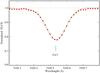 |
Fig. A.1 Synthetic profile of the Cu i5105 Å line for G05-40 from UVES spectra. The observed spectrum and theoretical synthesis are represented by red filled circles and the solid line, respectively. |
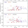 |
Fig. A.2 Distribution of line-to-line scatter as a function of metallicity for LTE abundances (bottom panel) and non-LTE abundances (top panel). The stars whose copper abundances were derived by only one line are not plotted in the figure. The symbols are as same as in Fig. 2. |
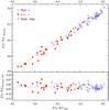 |
Fig. A.3 Comparison between this work and NS11 for the LTE results. The symbols are the same as in Fig. 2. |
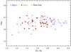 |
Fig. A.4 Distribution of surface gravity as a function of metallicity. The symbols are as same as in Fig. 2. |
LTE and non-LTE copper abundance ratios [Cu/Fe] for stars with VLT/UVES spectra.
LTE and non-LTE copper abundance ratios [Cu/Fe] for stars with NOT/FIES spectra.
All Tables
LTE and non-LTE copper abundance ratios [Cu/Fe] for stars with VLT/UVES spectra.
LTE and non-LTE copper abundance ratios [Cu/Fe] for stars with NOT/FIES spectra.
All Figures
|
Fig. 1 Departure coefficients bi of the selected energy levels (listed in the figure) as a function of continuum optical depth at 5000 Å for the model atmosphere of G05-40. The collision with neutral hydrogen was scaled by a factor of 0.1 following Shi et al. (2014). |
| In the text | |
|
Fig. 2 Abundance ratios [Cu/Fe] as a function of [Fe/H] for the program stars, where LTE and non-LTE results are represented in the left and right panel, respectively. The high-α (open blue circles), low-α (filled red circles) and thick-disk populations (black crosses) are indicated (see the online version for color copies of the figures). G112-42 and G112-43 are connected with a straight line. |
| In the text | |
|
Fig. 3 Differences in [Cu/Fe] between non-LTE and LTE as a function of metallicity (top panel), effective temperature (middle panel), and surface gravity (bottom panel). The symbols are the same as in Fig. 2. |
| In the text | |
|
Fig. A.1 Synthetic profile of the Cu i5105 Å line for G05-40 from UVES spectra. The observed spectrum and theoretical synthesis are represented by red filled circles and the solid line, respectively. |
| In the text | |
|
Fig. A.2 Distribution of line-to-line scatter as a function of metallicity for LTE abundances (bottom panel) and non-LTE abundances (top panel). The stars whose copper abundances were derived by only one line are not plotted in the figure. The symbols are as same as in Fig. 2. |
| In the text | |
|
Fig. A.3 Comparison between this work and NS11 for the LTE results. The symbols are the same as in Fig. 2. |
| In the text | |
|
Fig. A.4 Distribution of surface gravity as a function of metallicity. The symbols are as same as in Fig. 2. |
| In the text | |
Current usage metrics show cumulative count of Article Views (full-text article views including HTML views, PDF and ePub downloads, according to the available data) and Abstracts Views on Vision4Press platform.
Data correspond to usage on the plateform after 2015. The current usage metrics is available 48-96 hours after online publication and is updated daily on week days.
Initial download of the metrics may take a while.