| Issue |
A&A
Volume 585, January 2016
|
|
|---|---|---|
| Article Number | A111 | |
| Number of page(s) | 8 | |
| Section | Stellar structure and evolution | |
| DOI | https://doi.org/10.1051/0004-6361/201527315 | |
| Published online | 05 January 2016 | |
The long-period variables in ω Centauri⋆
1
Institute for Astrophysics (IfA), University of Vienna,
Türkenschanzstrasse 17,
1180
Vienna,
Austria
e-mail: This email address is being protected from spambots. You need JavaScript enabled to view it.
2
Australian National University, 0200
Canberra,
Australia
e-mail: This email address is being protected from spambots. You need JavaScript enabled to view it.
Received:
5
September
2015
Accepted:
22
October
2015
Abstract
Context. Recent studies have detected multiple populations in globular clusters. The massive globular cluster ω Cen hosts at least three populations of different metallicity. The most metal-rich one is thought to show also an overabundance of He. These differences should become visible in the structure, evolution, and pulsation of its stars.
Aims. We aim to study the effects of the different starting compositions of the three populations in ω Cen on the most luminous red giants in this cluster.
Methods. The long-periodic variability of evolved stars in ω Cen opens a comparably easy access window to the structure and composition of these objects. We made a detailed search for long-period variables (LPVs) in ω Cen leading to the detection of many new variables and period determinations for a significant number of them. Periods and luminosities were then compared with the most recent pulsation models for these kinds of stars.
Results. Some of the LPVs belong to each of the main metallicity sub-groups of ω Cen. Almost all detected variables with periods are fundamental mode pulsators. For the metal-rich group, our comparison with pulsation models favours a high He abundance of Y = 0.4.
Conclusions. Our study can be considered an independent piece of evidence supporting a high helium abundance among the metal-rich stars in ω Cen.
Key words: stars: AGB and post-AGB / stars: variables: general / globular clusters: individual: ωCentauri
Tables 3 and 4 are only available at the CDS via anonymous ftp to cdsarc.u-strasbg.fr (130.79.128.5) or via http://cdsarc.u-strasbg.fr/viz-bin/qcat?J/A+A/585/A111
© ESO, 2016
1. Introduction
Highly evolved stars on the upper part of the red giant branch (RGB) and the asymptotic giant branch (AGB) show a characteristic variability with a large amplitude light change at periods between approximately 30 to several hundred days. These stars are known as long-period variables (LPVs). The periodic pattern of variability is modified by variations in period length, multiple periods, and phases of irregular behaviour. Studies of field stars in the Magellanic Clouds (MCs) show that these pulsating stars fall on at least five major parallel period-luminosity (PL) relations, each relation corresponding to a different dominant pulsation mode. For recent discussions of the PL relations of LPVs we refer to Soszyński et al. (2013) and Wood (2015). Because of the diverse masses and compositions of MC field stars, it is difficult to understand exactly which modes occur at which luminosity for a given mass and metallicity. One way around this problem is to study red variables in clusters where all AGB stars have similar ages and usually similar metallicities as well.
We have used this approach in several earlier studies. In Lebzelter & Wood (2005), we investigated giant branch variables in the relatively metal-rich Galactic cluster 47 Tuc, showing that a switch occurs from higher to lower order modes as the stars increase in luminosity during their evolution on the giant branch. This finding was confirmed for the intermediate-age MC clusters NGC 1846 (Lebzelter & Wood 2007), NGC 1978, and NGC 419 (Kamath et al. 2010). Furthermore, using pulsation theory, Lebzelter & Wood (2005) and Kamath et al. (2010) showed that the red giants lost a substantial amount of mass as they evolved up the giant branch. In our most recent study (Lebzelter & Wood 2011) of the two clusters NGC 362 and NGC 2808, we investigated the effect of an increased helium abundance on the pulsation periods. Together with further studies on other clusters (Sahay et al. 2014a,b), we have collected an extensive sample of well characterized LPVs of different chemical composition. In total, the study of the PL diagrams in these clusters has provided an independent indicator of mass loss on the giant branch and potentially of He enrichment.
As an extension of this study we selected the peculiar Galactic globular cluster ω Cen (NGC 5139). This massive (D’Souza & Rix 2013) and well studied cluster became famous as one of the first ones showing a widened giant branch due to a wide spread in metallicity (e.g. Persson et al. 1980; Suntzeff & Kraft 1996). This indicated a complex history of the cluster, which is the product of either a merger event (Lee et al. 1999) or self-enrichment (Smith et al. 2000). Norris et al. (1997) showed a relation between kinematics and metallicity of the stars in ω Cen without being able to solve the mystery of the origin of the cluster’s multiple populations. Further studies (Bedin et al. 2004) have revealed a similar complexity on the subgiant branch and the main sequence. Norris (2004) suggests that there is a significant spread in the helium abundance among the various populations identified on the basis of metallicity. Studies of the main sequence show a dominant population with a normal helium abundance Y ≈ 0.25 and metallicity [Fe/H] ≈−1.6 and a smaller population with a high helium abundance Y ≈ 0.39 and metallicity [Fe/H] ≈−1.3 (Piotto et al. 2005; King et al. 2012). A first direct evidence for a He enhancement in ω Cen stars with [Fe/H] >−1.8 has been provided by observations of the prominent He I line near 1 μm by Dupree et al. (2011).
At least three different metallicity groups have been identified in ω Cen, a metal-rich one, a group with intermediate metallicity, and a metal poor population, where the latter two might show further substructure (Sollima et al. 2005; Gratton et al. 2011). The intermediate group includes the majority of the cluster stars and is very centrally concentrated. About one third of the stars belongs to the metal-poor group. The metal-rich group seems to be the smallest group within ω Cen.
The recent study by Villanova et al. (2014) distinguishes five different groups on the subgiant branch. These authors propose that ω Cen started with two populations, the high and the low metallicity group, likely resulting from a merger event and separated in age by several Gyr. Further evolution of each of the two initial populations then led to the situation observed today.
The interest in solving the mystery of ω Cen’s complex history resulted in an extensive set of stellar parameter and abundance determinations for red giants in this cluster. The most extensive abundance studies have been presented by Suntzeff & Kraft (1996), Johnson & Pilachowski (2010), and Simpson & Cottrell (2013). A large fraction of the cluster’s giants can thus be easily attributed to one of the three main groups based on the abundance pattern. In this paper we inspect the three groups in the light of their variability behaviour. A particular interest is seeing if pulsation properties can be used as an independent test for a high He abundance in any of the three metallicity groups.
Due to its brightness and prominence, ω Cen has been the target for various searches for variable stars in the past. However, a conclusive study dedicated to the variables on the upper giant branch is still missing. While various definitions for long-time variability are found in the searches for variable stars in this cluster, we will exclusively focus here on stars with periods exceeding 25 d and colours identifying them as red stars.
One of the oldest searches for variables is the work by Martin (1938) which includes also several red variables in the field of this cluster, among them the large amplitude variable V2 which is, however, probably a field star (van Leeuwen et al. 2000). Several of these objects have been further studied by Dickens et al. (1972), including velocity measurements to study their cluster membership. van Leeuwen et al. (2000), from a study of 100 plates obtained over several years, derived periods for 16 variables with periods longer than 25 d and gave membership probabilities based on proper motion. A more recent search, leading also to the detection of several candidates for long-period variability, was done by Kaluzny et al. (2004). In total, the Catalogue of Variable Stars in Galactic Globular Clusters (Clement et al. 2001)1 lists 14 long-period variables (classes SR and M), three of which are likely field stars. In addition, there are two stars listed as “L?” with unknown light curve parameters which may be seen as candidates for long-period variability (V394 and V396). The catalogue of Clement et al. (2001) does not include five stars listed as slowly varying stars by van Leeuwen et al. (2000): V53 and V162 have been reported as non-variable by Dickens et al. (1972). V165 is classified as an RR Lyr star in Clement et al. (2001) while van Leeuwen et al. (2000) give a period of 86.8 d. Finally, LEID 37110 (P = 68 d) and LEID 39105 (P = 71.5 d) are mentioned only as candidates in the catalogue (LEID is the Leiden number used by van Leeuwen et al. 2000).
2. Observations and data analysis
We obtained time series photometry of the red giants in ω Cen using the 2.0 m Faulkes Telescope South (Siding Spring Observatory), which is part of the Las Cumbres Observatory Global Telescope Network (Brown et al. 2013). Our time series covers almost two years starting in January 2011. The sampling rate varied over the year between three times per week to two times per month. This sampling ensured appropriate coverage for periods between 30 and 300 days. Observations were done in service mode. In total we were able to get 62 frames of sufficient quality in two filters, Bessell V and I. The images were taken with the Spectral Camera which gives a 10.5 × 10.5 arcmin field of view centred at the cluster centre with 0.3 arcsec pixels (double binned). Integration times were set to 30 s in V and 6 s in I. This allowed to us to study stars down to about V = 15.5 mag which corresponds to the lower brightness end of the horizontal branch. Photometric calibration was done using a set of standard stars in the field of RU 147 (Landolt 1992). In Fig. 1 we present a colour-magnitude diagram derived from our observations with the horizontal branch, the RGB, and the AGB clearly visible.
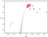 |
Fig. 1 V vs. V − I colour–magnitude diagram for stars in our observed field of ω Cen, using our values of V and I. LPVs (from Table 1) are marked by solid red squares. LPVs outside our observed field (from Table 2) are shown as open squares, using V and I values from Bellini et al. (2009). |
LPVs observed in ω Cen.
As in previous studies of this series, we used the image subtraction code ISIS 2.2 (Alard 2000) to search for variable stars in our V band time series. For a more detailed description we refer to Lebzelter & Wood (2005). Since we could not solve problems with applying ISIS 2.2. to the I band data, we decided to do PSF fitting photometry frame by frame using a code written by Ch. Alard and described in Schuller et al. (2003). For the V band, from consecutive nights we estimate a typical measurement error of ±0.01 magnitudes for LPVs. The uncertainty in I is slightly larger. Therefore, we defined our detection threshold for variability at a minimum amplitude of 0.05 mag in V. We selected only those variables that varied on time scales of 25 d or more. Period searches on the extracted light curves were done using the Fourier analysis code Period04 (Lenz & Breger 2005). Typically, periods derived from V band data were found in excellent agreement with periods from I band data. As a consequence of this and considering our sampling rate, we estimate a period uncertainty of less than 5% during the time span of the observations.
Data for LPVs in ω Cen outside our field of observation.
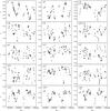 |
Fig. 2 V light curves of the LPVs in Table 1 for which a period could be determined. The lines show the fits to the light curves. Note that V129 is not a member of the cluster. |
3. Results
3.1. Variables
We detected 26 new long-period variables and confirmed the variability of eight previously known variables. All variables measured by our monitoring are listed in Table 1. In Table 2 we summarize the information about the previously-known LPVs in ω Cen (see Sect. 1) that are outside our field of observation. For the new detections we used the same naming scheme as in Lebzelter & Wood (2005). Since many variables showed significant irregularities or multiperiodicity in their light curves, the time span covered by our monitoring turned out to be too short to determine a clear periodicity for them. We have given only the well-determined periods in Table 1. The V magnitudes and V − I colours are mean values derived from our light curve data. Δ V is defined as the maximum peak-to-peak amplitude observed (rounded to the tenth of a magnitude). This amplitude includes variability due to the long secondary periods notable in some of our stars (e.g. LW16). The V light curves of all variables for which a period could be determined are presented in Fig. 2 together with the fit to the light curves. The V light curves of the stars for which no period could be determined are shown in Fig. 3. The epoch photometry in the V-band has been made available at the CDS2.
For five stars we can do a comparison of our period determination with the values given in the literature: There is an excellent agreement for V42, V138, and LEID 37110. For V152, our period is about 13% shorter than the value determined by van Leeuwen et al. (2000). The period given by Martin (1938) is 124 d. This might indicate that V152 is changing its pulsation period, maybe due to an evolutionary effect. The difference seen for V6 is quite large (154 d now, 110 d previously). However, the fit to our data is very convincing and does not allow for a period of 110 d. Testing our period of 154 d on the Kaluzny et al. (2004) light curve gave an acceptable fit as well. Therefore, we think that 154 d is the correct period for V6. Finally, we mention the star V129. According to the proper motion study of van Leeuwen et al. (2000), this star does not belong to ω Cen. Its colour, period and brightness make a classification as a foreground LPV very likely. Interestingly, the star shows also a long secondary period of approximately 470 d.
3.2. Additional data for the LPVs in ω Cen
In this section we discuss additional data available in the literature for the LPVs in ω Cen, starting with membership information. The most extensive search for ω Cen cluster members is probably the one by van Leeuwen et al. (2000). They used two sets of photographic plates from the 1930s and the 1970s to measure proper motions for stars down to 16th photographic magnitude. The resulting membership probability is listed in column 13 of Table 1. As noted previously, V129 is likely a non-member but all other variables detected in our survey have a high membership probability based on proper motion. In the case of ω Cen, stellar radial velocity is also an excellent indicator of membership since the cluster’s velocity is very high at ~233 km s-1, e.g. Sollima et al. (2009). In the extensive studies of Reijns et al. (2006) and van Loon et al. (2007) we find velocity measurements for 24 of the stars listed in Table 1, all in agreement with the cluster velocity except the non-member V129. Among them are LW7 and LW23 which show a slightly lower membership probability from the proper motion study, but they can safely be assumed to be cluster members based on their radial velocities. The membership of V42, doubted in Clement et al. (2001, see Table 2, seems to be confirmed both by proper motion and velocity measurements by Dickens et al. (1972) and van Loon et al. (2007). The latter paper also provides support for the membership of V6, V17, V53, V162, and V164. For the variables V186, V293, and V391 from Table2, the velocity measurements of Reijns et al. (2006) support their cluster membership.
Metallicity measurements are available for a large sample of ω Cen stars including all the variables listed in Table 1. We focused on two of the more recent literature sources, namely the papers by Johnson & Pilachowski (2010) and Simpson & Cottrell (2013) in order to get metallicity estimates for the variables. Their findings are given in Cols. 12 and 11 of Table 1, respectively. For the ω Cen LPVs outside our field of observations, we give the [Fe/H] values from these two surveys in Table 2.
Simpson & Cottrell (2013) based their [Fe/H] measurements on spectra from van Loon et al. (2007) with a resolution of R = 1600. They give a typical uncertainty of ±0.2 dex. The [Fe/H] values presented by Johnson & Pilachowski (2010) were derived from R = 18 000 spectra, and these authors give a maximum error of ±0.2 dex. While a comparison of the two metallicity measurements for our target stars reveals some differences between the two studies, there is an agreement within the error bars in most cases (Table 1). Since the work by Johnson & Pilachowski (2010) includes a larger fraction of our LPVs and since their study is based on spectra with the higher spectral resolution, we have used their metallicity values preferentially in our later analysis and we use the Simpson & Cottrell (2013) values only in cases where we have no measurements from Johnson & Pilachowski (2010) (LEID 39105 does not have a metallicity measurements from either Johnson & Pilachowski (2010) or Simpson & Cottrell (2013) so we use the [Fe/H] value from Norris & Da Costa (1995) for this star). Inspection of the [Fe/H] values in Tables 1 and 2 reveals that our LPVs include representatives of the three main metallicity groups detected in this cluster (see Sect. 1).
4. The ω Cen LPVs in the (Ks, J – Ks) diagram
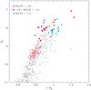 |
Fig. 4 Ks vs. J − Ks colour–magnitude diagram of stars on the upper giant branch of ω Cen. Known LPVs from Tables 1 and 2 are marked by large circles while smaller points are stars in a box of side 500 arcsec centred on the cluster and corresponding approximately to the field we monitored for LPVs. For the LPVs, values of [Fe/H] from Tables 1 and 2 were used to colour the circles according to the key shown on the figure. For stars not known to be variable, when an estimate of [Fe/H] existed from Suntzeff & Kraft (1996), this metallicity was used to colour the smaller circle. |
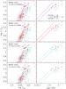 |
Fig. 5 (log Teff, log L) and (log P, log L) diagrams for stars in ω Cen (points) along with model fits to the diagrams (lines). The point colours are as in Fig. 4 and the abundances used to compute the model lines are shown in the panels at each vertical level. Solid lines are for stars on the RGB and dotted lines are for stars on the AGB. Note that models with abundances given in the bottom panels do not reach the AGB. In the right panels, lines corresponding to the radial fundamental and first-overtone modes are shown. |
Although a large number of studies exist on the various parts of ω Cen’s colour–magnitude diagram, little is known about the LPV population at the tip of the giant branch. In Fig. 4 we plot a Ks vs. (J − Ks) diagram based on 2MASS data (Skrutskie et al. 2006) for stars on the upper part of the giant branch. The points indicating each of the known LPVs are coloured according to the range of [Fe/H] to which they belong. For each non-variable star, when a metallicity estimate exists in Suntzeff & Kraft (1996), it is used to colour its point in the plot. We note that the [Fe/H] estimates of Johnson & Pilachowski (2010) and Suntzeff & Kraft (1996) agree quite well on average for non-variable red giants, with [Fe/H](Johnson & Pilachowski 2010)−[Fe/H] (Suntzeff & Kraft 1996) = 0.076 ± 0.155.
There is a general increase in (J − Ks) with increasing metallicity in Fig. 4, as expected from evolutionary tracks. The one very deviant point is LW23 (the purple point at (J − Ks) = 0.97 and Ks = 8.48) for which Simpson & Cottrell (2013) give [Fe/H] = −1.9, slightly below the metallicity limit of [Fe/H] = −1.8 for the red points. In fact, van Loon et al. (2007) give [Fe/H] = −1.75 for this star, which would make it a red point.
The most common stars on the luminous part of the giant branch above Ks = 10 have −1.8< [Fe/H] <−1.4. We note that the range −1.8< [Fe/H] <−1.4 corresponds to the most common population of ω Cen stars in general, and these stars form the red part of the main sequence below the turnoff. The next most common abundance group on the giant branch has [Fe/H] >−1.4 which corresponds to the stars belonging to the blue component of the main sequence. The main sequence position in the HR–diagram of this latter group of stars can only be explained by a very high helium abundance of Y ≈ 0.39 (e.g. King et al. 2012). The stars on the giant branch having [Fe/H] >−1.4 might also be expected to have a very high helium abundance.
5. Modelling the period–luminosity diagram
Figure 5 shows the (log Teff, log L) and (log P, log L) diagrams for stars in ω Cen. The 2MASS J − Ks and Ks values for each star were used to compute log Teff and log L. We adopted a mean reddening to ω Cen of E(B − V) = 0.11 (Calamida et al. 2005), the interstellar extinction law of Cardelli et al. (1989) and a true distance modulus of 13.7 (Del Principe et al. 2006). The transformations and bolometric corrections given in Houdashelt et al. (2000a,b) were then used to convert the de-reddened J − Ks and Ks to log Teff and log L.
Pulsation models designed to match the observations were computed with the code described in Wood (2015) using a mixing-length of 1.6 pressure scale heights. Metal abundances of Z = 0.00025, 0.0005 and 0.001 were used to approximately match the three observed metallicity groups [Fe/H] <−1.8, −1.8 < [Fe/H] <−1.4 and [Fe/H] >−1.4. Models were made with a helium mass fraction of Y = 0.25 for each of the three metal abundances and at the high metal abundance they were also made with a high helium abundance of Y = 0.40. Opacities at low temperatures were generated for each abundance using the online code of Marigo & Aringer (2009) and at high temperatures using the online OPAL codes (Iglesias & Rogers 1996). Scaled solar mixtures were used in all opacity tables. Masses of the models were computed assuming an age for ω Cen of 12 Gyr and a Reimers mass loss law (Reimers 1975) with multiplicative factor η = 0.33. The stellar evolution calculations of Bertelli et al. (2008) were used to estimate the mass at low luminosities on the RGB for an age of 12 Gyr, as well as to estimate the rate of evolution up the RGB and AGB, and to give the core mass during evolution. For the models with Y = 0.25, the mass of stars at low luminosities on the RGB is close to 0.8 M⊙ while for the models with Y = 0.40 this mass is close to 0.65 M⊙. For the latter models, mass loss on the RGB and a relatively large core mass means that the stars do not ascend the AGB after core helium burning.
The observational points in the HR-diagram (left panels of Fig. 5) show a decrease in Teff with increased metallicity, as also seen in Fig. 4. The model tracks for each abundance fit the corresponding observational points quite well, although at the highest luminosities the (purple) track for the lowest metallicity lies on the cool edge of the observational points. Note that for both Z = 0.00025 and 0.0005, one of the variables lies above the RGB tip for that metallicity suggesting that the most luminous variable lies on the AGB. For Z = 0.001, one of the variables lies above the tip of the RGB track for Y = 0.40. Since for Y = 0.40 there is no AGB, we conclude that this luminous variable must have a lower helium abundance since the evolutionary track for Y = 0.25 and Z = 0.001 can explain the most luminous variable as either an RGB or AGB star. This star shows that not all the stars belonging to the metal-rich population in ω Cen are He-enhanced. This result is consistent with the study of RR Lyrae variables in ω Cen by Marconi et al. (2011) which suggested that the He-enhanced population in the cluster cannot be larger than 20% of the horizontal branch population.
The observed periods of the LPVs in ω Cen are shown in the right panels of Fig. 5, with colour coding according to the observed metallicity. All the variables with periods in Tables 1 and 2 are plotted (except the likely non-member V129). Where periods are available from multiple sources, we use our own period as the first preference and the period from van Leeuwen et al. (2000) otherwise. The two variables V164 and V391 are omitted due to their very uncertain periods.
The model fundamental mode periods seem to fit the observed periods quite well at each metallicity. There appears to be only one variable with a determined period which is consistent with first-overtone pulsation: this is the shortest period variable (LW20) in the most metal-rich group with [Fe/H] >−1.4.
For the variables with [Fe/H] >−1.4, models were made with helium mass fractions of both Y = 0.25 and Y = 0.4. Increasing the helium abundance shifts the PL relation for LPVs to longer periods and the Y = 0.4 relation clearly fits the observations better than the Y = 0.25 relation. This suggests at least some of the metal-rich stars in ω Cen are indeed helium rich, as suggested by main-sequence isochrones. The longest period LPVs at a given luminosity are the most likely to be He-enhanced.
6. Summary and conclusions
We have monitored the globular cluster ω Cen over nearly 600 days with the aim of finding long-period variables and determining their periods of pulsation. We detected 26 new long-period variables, determined periods for nine of them, confirmed the variability of eight previously known variables and derived new periods for six of the previously known variables. Some of the LPVs belong to each of the main metallicity sub-groups of ω Cen viz. [Fe/H] <−1.8, −1.8 < [Fe/H] <−1.4 and [Fe/H] >−1.4. We made pulsation models for variables with abundances appropriate for each of the metallicity sub-groups. The model PL relations for radial fundamental mode pulsation fit the observed PL relations quite
well for each abundance sub-group. Only one star among those for which periods have been determined is a likely first-overtone pulsator. For the metal-rich group, the PL relation for stars with a high He abundance of Y = 0.4 is a better fit to the observations than the PL relation for stars with a normal helium abundance of Y = 0.25. This result can be considered an independent piece of evidence supporting a high helium abundance among the metal-rich stars in ω Cen.
See updates to this catalogue at http://www.astro.utoronto.ca/~cclement/read.html
Table 3 at the CDS includes the data for the stars shown in Fig. 2, and Table 4 the ones presented in Fig. 3. The first column of each table gives the Julian Date and the following columns give the V photometry for the variables in the same order as shown in the figures – see the ReadMe file at the CDS.
Acknowledgments
The work of T.L. has been supported by the Austrian Science Fund FWF under project number P23737. This publication makes use of data products from the Two Micron All Sky Survey, which is a joint project of the University of Massachusetts and the Infrared Processing and Analysis Center/California Institute of Technology, funded by the National Aeronautics and Space Administration and the National Science Foundation.
References
- Alard, C. 2000, A&AS, 144, 363 [NASA ADS] [CrossRef] [EDP Sciences] [Google Scholar]
- Bedin, L. R., Piotto, G., Anderson, J., et al. 2004, ApJ, 605, L125 [NASA ADS] [CrossRef] [Google Scholar]
- Bellini, A., Piotto, G., Bedin, L. R., et al. 2009, A&A, 493, 959 [NASA ADS] [CrossRef] [EDP Sciences] [Google Scholar]
- Bertelli, G., Girardi, L., Marigo, P., & Nasi, E. 2008, A&A, 484, 815 [NASA ADS] [CrossRef] [EDP Sciences] [Google Scholar]
- Brown, T. M., Baliber, N., Bianco, F. B., et al. 2013, PASP, 125, 1031 [NASA ADS] [CrossRef] [Google Scholar]
- Calamida, A., Stetson, P. B., Bono, G., et al. 2005, ApJ, 634, L69 [NASA ADS] [CrossRef] [Google Scholar]
- Cardelli, J. A., Clayton, G. C., & Mathis, J. S. 1989, ApJ, 345, 245 [NASA ADS] [CrossRef] [Google Scholar]
- Clement, C. M., Muzzin, A., Dufton, Q., et al. 2001, AJ, 122, 2587 [NASA ADS] [CrossRef] [Google Scholar]
- Del Principe, M., Piersimoni, A. M., Storm, J., et al. 2006, ApJ, 652, 362 [NASA ADS] [CrossRef] [Google Scholar]
- Dickens, R. J., Feast, M. W., & Lloyd Evans, T. 1972, MNRAS, 159, 337 [NASA ADS] [CrossRef] [Google Scholar]
- D’Souza, R., & Rix, H.-W. 2013, MNRAS, 429, 1887 [NASA ADS] [CrossRef] [Google Scholar]
- Dupree, A. K., Strader, J., & Smith, G. H. 2011, ApJ, 728, 155 [NASA ADS] [CrossRef] [MathSciNet] [Google Scholar]
- Gratton, R. G., Johnson, C. I., Lucatello, S., D’Orazi, V., & Pilachowski, C. 2011, A&A, 534, A72 [NASA ADS] [CrossRef] [EDP Sciences] [Google Scholar]
- Houdashelt, M. L., Bell, R. A., & Sweigart, A. V. 2000a, AJ, 119, 1448 [Google Scholar]
- Houdashelt, M. L., Bell, R. A., Sweigart, A. V., & Wing, R. F. 2000b, AJ, 119, 1424 [NASA ADS] [CrossRef] [Google Scholar]
- Iglesias, C. A., & Rogers, F. J. 1996, ApJ, 464, 943 [NASA ADS] [CrossRef] [Google Scholar]
- Johnson, C. I., & Pilachowski, C. A. 2010, ApJ, 722, 1373 [NASA ADS] [CrossRef] [Google Scholar]
- Kaluzny, J., Olech, A., Thompson, I. B., et al. 2004, A&A, 424, 1101 [NASA ADS] [CrossRef] [EDP Sciences] [Google Scholar]
- Kamath, D., Wood, P. R., Soszyński, I., & Lebzelter, T. 2010, MNRAS, 408, 522 [NASA ADS] [CrossRef] [Google Scholar]
- King, I. R., Bedin, L. R., Cassisi, S., et al. 2012, AJ, 144, 5 [NASA ADS] [CrossRef] [Google Scholar]
- Landolt, A. U. 1992, AJ, 104, 340 [NASA ADS] [CrossRef] [Google Scholar]
- Lebzelter, T., & Wood, P. R. 2005, A&A, 441, 1117 [NASA ADS] [CrossRef] [EDP Sciences] [Google Scholar]
- Lebzelter, T., & Wood, P. R. 2007, A&A, 475, 643 [NASA ADS] [CrossRef] [EDP Sciences] [Google Scholar]
- Lebzelter, T., & Wood, P. R. 2011, A&A, 529, A137 [NASA ADS] [CrossRef] [EDP Sciences] [Google Scholar]
- Lee, Y.-W., Joo, J.-M., Sohn, Y.-J., et al. 1999, Nature, 402, 55 [NASA ADS] [CrossRef] [Google Scholar]
- Lenz, P., & Breger, M. 2005, Comm. Asteroseismol., 146, 53 [Google Scholar]
- Marconi, M., Bono, G., Caputo, F., et al. 2011, ApJ, 738, 111 [NASA ADS] [CrossRef] [Google Scholar]
- Marigo, P., & Aringer, B. 2009, A&A, 508, 1539 [NASA ADS] [CrossRef] [EDP Sciences] [Google Scholar]
- Martin, W. C. 1938, Annalen van de Sterrewacht te Leiden, 17, B1 [Google Scholar]
- Norris, J. E. 2004, ApJ, 612, L25 [NASA ADS] [CrossRef] [Google Scholar]
- Norris, J. E., & Da Costa, G. S. 1995, ApJ, 447, 680 [NASA ADS] [CrossRef] [Google Scholar]
- Norris, J. E., Freeman, K. C., Mayor, M., & Seitzer, P. 1997, ApJ, 487, L187 [NASA ADS] [CrossRef] [Google Scholar]
- Persson, S. E., Cohen, J. G., Matthews, K., Frogel, J. A., & Aaronson, M. 1980, ApJ, 235, 452 [Google Scholar]
- Piotto, G., Villanova, S., Bedin, L. R., et al. 2005, ApJ, 621, 777 [NASA ADS] [CrossRef] [Google Scholar]
- Reijns, R. A., Seitzer, P., Arnold, R., et al. 2006, A&A, 445, 503 [NASA ADS] [CrossRef] [EDP Sciences] [Google Scholar]
- Reimers, D. 1975, in Circumstellar envelopes and mass loss of red giant stars, eds. B. Baschek, W. H. Kegel, & G. Traving, 229 [Google Scholar]
- Sahay, A., Lebzelter, T., & Wood, P. 2014a, IBVS, 6107, 1 [NASA ADS] [Google Scholar]
- Sahay, A., Lebzelter, T., & Wood, P. R. 2014b, PASA, 31, 12 [NASA ADS] [CrossRef] [Google Scholar]
- Schuller, F., Ganesh, S., Messineo, M., et al. 2003, A&A, 403, 955 [NASA ADS] [CrossRef] [EDP Sciences] [Google Scholar]
- Simpson, J. D., & Cottrell, P. L. 2013, MNRAS, 433, 1892 [NASA ADS] [CrossRef] [Google Scholar]
- Skrutskie, M. F., Cutri, R. M., Stiening, R., et al. 2006, AJ, 131, 1163 [NASA ADS] [CrossRef] [Google Scholar]
- Smith, V. V., Suntzeff, N. B., Cunha, K., et al. 2000, AJ, 119, 1239 [NASA ADS] [CrossRef] [Google Scholar]
- Sollima, A., Pancino, E., Ferraro, F. R., et al. 2005, ApJ, 634, 332 [NASA ADS] [CrossRef] [Google Scholar]
- Sollima, A., Bellazzini, M., Smart, R. L., et al. 2009, MNRAS, 396, 2183 [NASA ADS] [CrossRef] [Google Scholar]
- Soszyński, I., Wood, P. R., & Udalski, A. 2013, ApJ, 779, 167 [NASA ADS] [CrossRef] [Google Scholar]
- Suntzeff, N. B., & Kraft, R. P. 1996, AJ, 111, 1913 [NASA ADS] [CrossRef] [Google Scholar]
- van Leeuwen, F., Le Poole, R. S., Reijns, R. A., Freeman, K. C., & de Zeeuw, P. T. 2000, A&A, 360, 472 [NASA ADS] [Google Scholar]
- van Loon, J. T., van Leeuwen, F., Smalley, B., et al. 2007, MNRAS, 382, 1353 [NASA ADS] [CrossRef] [Google Scholar]
- Villanova, S., Geisler, D., Gratton, R. G., & Cassisi, S. 2014, ApJ, 791, 107 [NASA ADS] [CrossRef] [Google Scholar]
- Wood, P. R. 2015, MNRAS, 448, 3829 [NASA ADS] [CrossRef] [Google Scholar]
All Tables
All Figures
|
Fig. 1 V vs. V − I colour–magnitude diagram for stars in our observed field of ω Cen, using our values of V and I. LPVs (from Table 1) are marked by solid red squares. LPVs outside our observed field (from Table 2) are shown as open squares, using V and I values from Bellini et al. (2009). |
| In the text | |
|
Fig. 2 V light curves of the LPVs in Table 1 for which a period could be determined. The lines show the fits to the light curves. Note that V129 is not a member of the cluster. |
| In the text | |
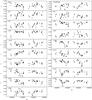 |
Fig. 3 V light curves of the LPVs in Table 1 for which a period could not be determined. |
| In the text | |
|
Fig. 4 Ks vs. J − Ks colour–magnitude diagram of stars on the upper giant branch of ω Cen. Known LPVs from Tables 1 and 2 are marked by large circles while smaller points are stars in a box of side 500 arcsec centred on the cluster and corresponding approximately to the field we monitored for LPVs. For the LPVs, values of [Fe/H] from Tables 1 and 2 were used to colour the circles according to the key shown on the figure. For stars not known to be variable, when an estimate of [Fe/H] existed from Suntzeff & Kraft (1996), this metallicity was used to colour the smaller circle. |
| In the text | |
|
Fig. 5 (log Teff, log L) and (log P, log L) diagrams for stars in ω Cen (points) along with model fits to the diagrams (lines). The point colours are as in Fig. 4 and the abundances used to compute the model lines are shown in the panels at each vertical level. Solid lines are for stars on the RGB and dotted lines are for stars on the AGB. Note that models with abundances given in the bottom panels do not reach the AGB. In the right panels, lines corresponding to the radial fundamental and first-overtone modes are shown. |
| In the text | |
Current usage metrics show cumulative count of Article Views (full-text article views including HTML views, PDF and ePub downloads, according to the available data) and Abstracts Views on Vision4Press platform.
Data correspond to usage on the plateform after 2015. The current usage metrics is available 48-96 hours after online publication and is updated daily on week days.
Initial download of the metrics may take a while.