| Issue |
A&A
Volume 585, January 2016
|
|
|---|---|---|
| Article Number | A25 | |
| Number of page(s) | 8 | |
| Section | Extragalactic astronomy | |
| DOI | https://doi.org/10.1051/0004-6361/201526071 | |
| Published online | 09 December 2015 | |
On the detectability of Lorentz invariance violation through anomalies in the multi-TeV γ-ray spectra of blazars
INAF–Osservatorio Astronomico di Brera, via E. Bianchi 46, 23807 Merate, Italy
e-mail: This email address is being protected from spambots. You need JavaScript enabled to view it.
Received: 11 March 2015
Accepted: 4 October 2015
Abstract
Context. Cosmic opacity for very high energy γ rays (E> 10 TeV) that result from the interaction with the extragalactic background light can be strongly reduced. This is because of possible Lorentz-violating terms in the dispersion relations for particles expected for several versions of quantum gravity theories.
Aims. We discuss the possibility of using very high-energy observations of blazars to detect anomalies in the cosmic opacity that are induced by Lorentz invariance violation (LIV), taking the possibility of using extreme BL Lacertae (BL Lac) objects into particular consideration, as well as the bright and nearby BL Lac Mkn 501.
Methods. We derive the modified expression for the optical depth of γ rays by also taking redshift dependence into consideration and, by applying this, we derive the expected high-energy spectrum above 10 TeV of Mkn 501, in high and low states, and of the extreme BL Lac 1ES 0229+200.
Results. Along with the nearby and well studied BL Lac Mkn 501 especially in high state, other suitable targets are extreme BL Lac objects, characterized by quite hard TeV intrinsic spectra which probably extend at the energies relevant when detecting LIV features.
Key words: BL Lacertae objects: individual: Mkn 501 / gamma rays: general / BL Lacertae objects: individual: 1ES 0229+200 / astroparticle physics
© ESO, 2015
1. Introduction
Both the standard model of particle physics and general relativity are thought to be the low-energy limits of a more fundamental physical theory. Efforts to build a comprehensive theory often lead to schemes in which the Lorentz invariance is violated at very high energies (e.g., Mattingly 2005; Liberati 2013). The effects related to Lorentz invariance violation (LIV) are likely to be greatly suppressed at low energy by terms of the order of (E/ELIV)n. In this instance, E is the considered energy and ELIV is the relevant energy scale, which is commonly assumed to be of the order of the Planck energy,  GeV. Although the effects induced by LIV are likely to be quite small at energies that are attainable by most of the current experiments, they can result in observable anomalies in processes that are characterized by well-defined energy thresholds. Indeed, LIV terms modify the standard energy-momentum relation and can induce variations in the kinematics of scattering and decay processes (e.g., Coleman & Glashow 1999; Jacobson et al. 2003). This allows for reactions that are forbidden by standard physics (e.g. photon decay) and can change energy thresholds, as in the case the γγ → e+e− pair production reaction (e.g. Kifune 1999; 2014; Protheroe & Meyer 2000).
The modification of the γγ → e+e− scattering can be probed effectively by observations of blazars at very high energy. Indeed, LIV effects in this reaction become relevant at energies 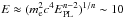 TeV for n = 3, i.e., the lowest order that is interesting for deviations in the high-energy regime. Gamma rays of these energies are effectively absorbed through the interaction with the low-energy radiation of the extragalactic background light (EBL). Deviations in the scattering kinematics that is induced by LIV can lead to the reduction of cosmic opacity, thus allowing high-energy photons (E> 10 TeV) to evade absorption and reach the Earth. The detection of such anomalies in opacity is still difficult since the performance of current TeV observatories do not allow us to obtain good quality spectra of blazars at energies above 10 TeV. The upcoming Cherenkov Telescope Array (CTA; Acharya et al. 2013) and its precursors, such as the proposed ASTRI/CTA mini array (Di Pierro et al. 2013), will greatly improve the sensitivity above 10 TeV, and provide ideal instruments to probe and constrain LIV scenarios1. The search for LIV effects based on the modification of the cosmic opacity is complementary to the method based on measuring energy-dependent photon time of flight from cosmic sources (Amelino-Camelia et al. 1998; Ellis & Mavromatos 2013). These were recently applied to GRB and blazars and already provide interesting lower limits for the LIV energy scale of photons, ELIV> 9.3 × 10¹⁹ GeV for n = 1 and ELIV> 1.3 × 10¹¹ GeV for n = 2 (Vasileiou et al. 2013). In fact, not all scenarios, including LIV, predict the same effects and thus different methods can probe LIV in different frameworks. Furthermore, while time-of-flight measurements only test LIV with photons, the method that is based on the modification of the kinematics of the γγ → e+e− reaction also involves Lorentz violating terms for the dispersion relations of the resulting leptons (Kifune 1999).
Recently, Fairbairn et al. (2014) performed a feasibility study on the possible detection of spectral LIV effects with high-energy observations of blazars by CTA, which was based on the expected opacity for different values of the LIV energy scale for photons. In this paper we extend their treatment to include the redshift dependence of the EBL and we compare this treatment to the one previously presented by Jacob & Piran (2008). We further proceed to discuss the targets most suitable for this study and propose that LIV effects could be constrained effectively through deep observations of the so-called extreme BL Lacs (EHBL; e.g. Costamante et al. 2001; Tavecchio et al. 2011; Bonnoli et al. 2015) that are located at relatively large redshift (z ~ 0.1−0.2). In Sect. 2, we review the calculation of the modified optical depth, extending the Fairbairn et al. (2014) treatment. In Sect. 3 we then discuss the best instances of blazars to use to probe for LIV using the opacity anomaly, and finally in Sect. 4, we draw our conclusions.
Throughout the paper, the following cosmological parameters are assumed: H0 = 70 km s-1 Mpc-1, ΩM = 0.3, ΩΛ = 0.7.
2. Gamma-ray absorption with LIV
Inspired by effective field theories and quantum gravity theories, the modifications that LIV introduces to reaction thresholds at high energy are commonly studied using phenomenological dispersion relations for the involved particles. Here the effects of LIV are expressed with the addition of terms in the form of  , where E is the particle energy (e.g., Kifune 1999). We limit the following treatment to the n = 1 case, for which the modified relation for photons reads
 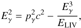 (1)where pγ is the photon momentum. The term
  acts as an effective mass term for photons and induces modifications of the threshold of the γγ → e+e− scattering for values of the energy for which the term becomes comparable to the threshold energy ≈ mec2. In principle, the LIV terms can assume different values for different particle species2 and can be both positive or negative. The sign assumed above is one where an interesting anomaly (i.e. decreasing opacity for increasing energy) is displayed for every value of ELIV. The ELIV term in the denominator – related to the energy scale of LIV effects – is generally assumed to be of the order of the Planck energy.
Calculating the modified optical depth, including LIV effects, is quite a delicate process since, in the LIV framework, even basic standard assumptions (e.g., energy-momentum conservation) could be invalid. In the literature, expressions for the optical depth, derived with two alternative assumptions, are given by Jacob & Piran (2008) and Fairbairn et al. (2014). In both works, the modified dispersion relation that is given in Eq. (1) is assumed, and the same modified expression for the minimum energy of the soft target photons that allow the pair-production reaction is found (see also Kifune 1999): 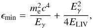 (2)where the last term is introduced by LIV effects. This expression can be obtained solely on the minimal assumption that the standard energy-momentum conservation still holds in a Lorentz-violating framework. (Note, however, that this may not be true in some LIV schemes, most notably in the so-called double special relativity, Amelino-Camelia et al. 2005.)
The resulting energy, ϵmin,, of target photons at the threshold for the reaction with γ rays with energy Eγ is shown in Fig. 1. The black solid line shows the standard value 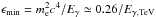 eV. The other lines indicate the modified threshold energy for different values of ELIV, normalized to the expected characteristic energy for LIV, ELIV = 1019 GeV. The common feature of the curves, including LIV effects, is the existence of a minimum for ϵmin, which corresponds to energies of the incoming γ ray around Ec = 30−50 TeV. The existence of the minimum implies a progressive reduction of the resulting optical depth above Ec. The curves, which correspond to the increasing value of ELIV (from ELIV = 1019 GeV to 2 × 10²⁰ GeV), track the progressive shift of Ec to higher energies.
The treatments of Jacob & Piran (2008) and Fairbairn et al. (2014) differ from the assumptions made to further derive the expression for the optical depth τγγ (see the Appendix for more details). Jacob & Piran (2008) assume the standard formula (e.g., Dweck & Krennrich 2012) and that the functional form of the cross-section, which in the standard case can be expressed as a function of the ratio ϵ/ϵmin, still holds at energies where LIV effects begin to be significant. It is worth noting that their procedure avoids any change of reference frame since any quantity is evaluated in the observer frame. The optical depth can thus be calculated with the standard expression.
Fairbairn et al. (2014), instead, used a modified expression for the square of the center-of-mass energy s, including the effective mass for the photon  ,
,  , in which θ is the angle between the two photon directions. They assumed that s continues to be a good invariant (see Jacob et al. 2010 for a justification of this assumption). They calculate the expected modification of the cosmic opacity for γ rays for close-by sources, for which the redshift and the EBL evolution can be safely neglected. In the following calculation of the optical depth, we use a redshift-dependent EBL density, which allows us to consider sources at arbitrary distances.
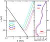 |
Fig. 1 Left: photon target energy at threshold ϵmin for the pair-production reaction as a function of the γ-ray energy Eγ. The black solid line shows the standard case. The other lines indicate the modified threshold, which result from the LIV-modified kinematics, for different values of the parameter ELIV (in units of 1019 GeV). Right: EBL (Dominguez et al. 2011, solid red; Kneiske & Dole 2010, solid blue) and CMB (dashed red) local density ϵn(ϵ) (horizontal axis) as a function of the energy ϵ (vertical axis), to be compared with the energy threshold in the left panel. |
The standard relation for optical depth at the energy Eγ and for a source at redshift zs (e.g., Dwek & Krennrich 2013) is modified as (Fairbairn et al. 2014) ![Mathematical equation: \begin{eqnarray} \tau_{\gamma\gamma}(E_{\gamma},z_{\rm s})&=&\frac{c}{8E_{\gamma}^2}\int_0^{z_{\rm s}} \frac{{\rm d}z}{H(z)(1+z)^3}\, \int_{\epsilon_{\rm min}(z)}^{\infty} \frac{n(\epsilon,z)}{\epsilon^2}{\rm d}\epsilon \nonumber \\ &&\times \int_{s_{\rm min}(z)}^{s_{\rm max}(z)} [s-m^2_{\gamma}(z)] \, \sigma _{\gamma\gamma}(s)\, {\rm d}s, \label{eq:tau} \end{eqnarray}](/articles/aa/full_html/2016/01/aa26071-15/aa26071-15-eq44.png) (3)where H(z) = H0 [ΩΛ + ΩM(1 + z)3] 1/2, ϵ is the target photon energy, n(ϵ,z) is the redshift-dependent differential EBL photon number density, and σγγ(s) is the total pair production cross section as a function of the modified square of the center of mass energy . The limits of the last integral reads
(3)where H(z) = H0 [ΩΛ + ΩM(1 + z)3] 1/2, ϵ is the target photon energy, n(ϵ,z) is the redshift-dependent differential EBL photon number density, and σγγ(s) is the total pair production cross section as a function of the modified square of the center of mass energy . The limits of the last integral reads 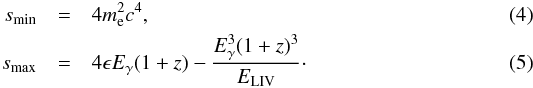 Standard relations are clearly recovered for ELIV → ∞. In Eq. (5) we neglect the energy-dependent speed of light βγ(Eγ) since, for the energies that are relevant here, βγ(Eγ) ≃ 1. The (1 + z) terms in Eqs. (4) and (5) take into account the progressive redshift of the γ rays while they propagate from the source to the Earth.
For the EBL density n(ϵ,z) we use two models, namely the state-of-the art model by Dominguez et al. (2011, D11 hereafter) and the model by Kneiske & Dole (2010, KD10). The latter model predicts a somewhat lower level of IR radiation, determining a smaller optical depth at energies above a few TeV. The local photon densities predicted by the two models are reported in the right hand panel of Fig. 1.
In Figs. 2 and 3 we report the absorption coefficient exp [−τγγ(Eγ)] (calculated with Eq. (3)) for two values of the redshift, z = 0.03 (upper panel) and 0.14 (lower panel) and the values of ELIV considered above, and the two different EBL models. The drastic reduction in the opacity above few tens of TeV induced by the LIV effect is clearly visible. In the top panel of Fig. 2 we also report the curves that correspond to optical depths that were evaluated using the method of Jacob & Piran (2008). Clearly, the results of the two methods differ only at the highest energies and the ratio between the two absorption coefficients is always less then a factor of two. For simplicity, hereafter we only report the results obtained with the Fairbairn et al. (2014) treatment. See the Appendix for more details.
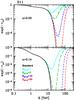 |
Fig. 2 Absorption coefficient e− τγγ as a function of energy for γ rays that propagate from a source at z = 0.03 (upper panel) and z = 0.14 (lower panel), using the EBL model of Dominguez et al. (2011). The black solid line indicates the standard case, the other lines show the modified coefficient for different values of ELIV (with the color code reported in the caption). Thick lines have been obtained using the treatment of Fairbairn et al. (2014). For comparison, thin lines show the results of the calculations that were based on the assumptions of Jacob & Piran (2008). |
3. Application to blazar spectra
An ideal source to test possible modifications of the γ-ray opacity induced by LIV should be a bright emitter above 20−30 TeV, at which the LIV effects become fully appreciable. Unfortunately, this requirement is in conflict with the typical characteristics of the VHE-emitting blazars. These commonly display (intrinsic) spectra softening with energy as a result of the decreasing inverse Compton scattering, particle acceleration efficiencies and, possibly, internal opacity. However, given the extreme variability that characterizes blazars, it is likely that some sources may display hard and bright TeV emission, which is particularly suitable for the present analysis. It is also becoming clear that a class of peculiar BL Lacs, known as “extreme” BL Lacs (Costamante 2001; Tavecchio et al. 2011; Bonnoli et al. 2015), are characterized by a very hard and stable TeV continuum, possibly extending above 10 TeV. The relatively high redshift of these sources (z> 0.1) implies a relatively large absorption, which is, however, greater than compensated for by the expected intrinsic flux above 20−30 TeV, where LIV effects become significant.
On this basis, in the following we investigate the prospects of probing LIV spectral effects using observations of high-states of Mkn 501, a classical TeV BL Lac object, as well as the prototype extreme, BL Lac 1ES 0229+200.
3.1. Mkn 501
Early studies (e.g., Kifune 1999; Protheroe & Meyer 2000) focus on the nearby and luminous BL Lac objects Mkn 501. The spectrum of this source during quiescent states has been also considered by Fairbairn et al. (2014) when investigating the CTA potential of detecting LIV. A problem with this and similar sources (e.g., Mkn 421) is the typical steep spectrum, which implies that the value of the intrinsic flux above 20−30 TeV is expected to be quite low. Moreover, current observations, limited to E ≲ 20 TeV, do not ensure that the emission continues at the required energies without breaks. A steepening or a cut-off of the emitted spectrum could indeed hamper or strongly limit the application of the method.
Interestingly, Mkn 501 occasionally shows active states in which the spectrum becomes remarkably hard (photon index ΓVHE ~ 2) and extends at least up to ~20 TeV. The most studied high state occurred in 1997 and for this state there is a superb quality spectrum recorded by HEGRA (Aharonian et al. 1999). Two other similar states were observed in 2009 and 2011, and VHE spectra were obtained by VERITAS (Abdo et al. 2011) and ARGO (Bartoli et al. 2012). As shown by Neronov et al. (2012) the hard TeV spectrum in 2009 was also accompanied by an exceptionally hard spectrum above 10 GeV that was detected by LAT (ΓLAT ~ 1). These active phases lasted for several weeks. Clearly, the spectral hardness and the high flux during these flaring states are ideal for studying LIV effects. Consequently, in the following we use the HEGRA 1997 spectrum.
In Fig. 4 we show our predictions for the observed spectrum at high energy during this activity state for the two EBL models. The choice of the spectral shape (a power law with exponential cut-off) is constrained by the requirement to reproduce the observed data points, assuming no LIV. In all cases, in the presence of LIV effects, the spectrum is predicted to show quite a narrow upturn, where the observed spectrum would recover to the intrinsic one. Clearly the predicted spectra for the D11 EBL model and the cases with ELIV = 1019 GeV and 3 × 10¹⁹ GeV are inconsistent with the observed data. Therefore, these data for Mkn 501 already suggest ELIV ≳ 3 × 10¹⁹ GeV.
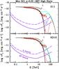 |
Fig. 4 Observed γ-ray spectrum of Mkn 501 during the 1997 active state recorded HEGRA (red symbols). The black solid and dotted orange lines show the observed and the intrinsic spectrum, assuming standard absorption with the D11 (upper panel) and KD10 (lower panel) EBL models. Grey points indicate the observed data points corrected for absorption. Other lines show the predicted spectrum with LIV effects (line styles and colors as in Fig. 2). The violet lines show the 5σ sensitivity curves for CTA (5 h, dashed and 50 h exposure, solid). |
By way of comparison, in Fig. 4 we show the expected differential 5σ sensitivity curves for CTA with an exposure time of 50 h (from Bernlöhr et al. 2013, model “SAM” in Fig. 14) and 5 h (derived from Fig. 8 in Bernlöhr et al. 2013). With the longest assumed exposure, in the D11 case, CTA should be able to reveal the LIV upturn easily, even for the largest assumed value of the photon LIV parameter, ELIV = 2 × 10²⁰ GeV. In the case of the KD10 EBL model, the required intrinsic spectrum has a cut-off at an energy lower than that found for the D11 case, since the absorption around 10 TeV is lower. In turn, a lower energy cut-off implies that the LIV upturn is much less pronounced, making it difficult to probe values of ELIV larger than ~ 1020 GeV
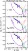 |
Fig. 5 Observed γ-ray spectrum of Mkn 501 during a quiescent phase (Acciari et al. 2011). The three panels report the received γ-ray spectrum for different assumed intrinsic spectra (from top to bottom: a simple power law with energy index α = 0.52; a power law with energy index α = 0.52 and an exponential cut-off with e-folding energy Ecut = 50 TeV; a cut-offed power law with α = 0.52 and Ecut = 15 TeV) and values of ELIV (color code as in Fig. 2). The HAWC and CTA sensitivity curves (as in Fig. 3) are displayed for an exposure time of one year and 50 h, respectively. |
In comparison, Figs. 5 and 6 report the case that corresponds to a low state, as assumed by Fairbairn et al. (2014). We note in passing that they incorrectly assume that the intrinsic spectral slope is that traced by the observed spectrum. On the contrary, as noted above, the optical depth cannot be neglected and, indeed, the intrinsic spectrum is harder than the observed one, with Δα ≃ 0.2. This is valid for both EBL models, since the observed datapoints cover an energy range for which the two models basically provide the same opacity. Once extrapolated at high-energy, the flux is thus larger than that which was assumed in Fairbairn et al. (2014): their results should thus be considered somewhat pessimistic. This is particularly important for the KD10 model, which provides a lower opacity, and thus a large flux, at energies where LIV effects are significant. We note the difference with the previous case of the high state, for which the observed spectrum extends up to energies where the KD10 opacity is lower and thus the predicted flux for LIV effects is lower than the D11 case.
Even with 50 h of observations, CTA can easily detect the spectral upturn for all parameters assumed here for the case in which the intrinsic emission follows an unbroken power law. If the spectrum exponentially drops with Ecut> 50 TeV, the upturn can still be detected in the most favorable cases. For smaller values of Ecut, the detection of the anomalous transparency is challenging. By way of comparison, we also report the differential sensitivity curve for an exposure of one year with HAWC (Abeysekara et al. 2013). In fact, quiescent states are likely to last for a long time and, thus, we can assume relatively long exposure times, which are also suitable for HAWC and other instruments (see Discussion).
3.2. Extreme highly peaked BL Lacs: 1ES 0229-200
As clearly seen in the last example, the effective investigation of LIV spectral anomalies benefits from hard spectra and large maximum energies. In view of these requirements, EHBL, characterized by quite hard TeV spectra that extend up to at least 10 TeV, should make good targets. However, the peculiar emission properties of these sources are still not clearly understood. EHBL are characterized by extremely low-radio luminosity, together with luminous and hard X-ray emission, which often locates the peak of the synchrotron emission above 10 keV (e.g. Bonnoli et al. 2015). The hardness of the VHE spectrum after correction for EBL absorption is challenging for the standard one-zone leptonic model, in which the inverse Compton scattering of multi-TeV electrons (which in this framework is responsible for the γ-ray emission) becomes quite inefficient (Katarzyński et al. 2006; Tavecchio et al. 2009; 2011; Kaufmann et al. 2011). Another peculiarity is related to the absent or very weak variability displayed by the VHE emission (e.g., Aliu et al. 2014), which is at odds with the typical extreme behavior of the bulk of the BL Lac population. Possible alternative explanations include hadronic emission (Cerutti et al. 2015; Murase et al. 2012), internal absorption (Zacharopoulou et al. 2011), or quasi-Maxwellian energy distribution of the emitting leptons (Lefa et al. 2011).
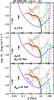 |
Fig. 7 Observed high-energy SED of 1ES 0229+200. Black symbols are LAT measurements from the 3FGL catalogue. Orange triangles indicate the HESS spectrum (Aharonian et al. 2007) while the gray triangles indicate fluxes that are obtained after correction for the absorption with EBL. The dotted line indicates the assumed intrinsic spectrum. The three panels report the received γ-ray spectrum for different assumed intrinsic spectra (from top to bottom: a simple power law with energy index α = 0.4; a broken power law with high-energy index α2 = 2 and break energy Eb = 10 TeV; an exponential cut-off with e-folding energy Ecut = 15 TeV) and values of ELIV (color code as in Fig. 2). The HAWC and CTA sensitivity curves (as in Fig. 3) are displayed for an exposure time of five years and 50 h, respectively. |
As a benchmark case, we consider 1ES 0229-200 (z = 0.14), which is a prototype for this class of sources (Tavecchio et al. 2009; Bonnoli et al. 2015). The relatively large redshift of 1ES 0229-200 implies an important absorption of the VHE spectrum. The observed spectrum is indeed soft (Γ ≃ 2.5) but, when corrected for (standard) absorption, results in very hard continuum that remains apparently unbroken up to 10 TeV (Aharonian et al. 2007). In Figs. 7 and 8, together with the observed data points and those with the correction for absorption within, for? the two EBL models, we present the prediction for the high-energy spectrum based on three possible intrinsic spectral shapes that are compatible with the observed data, namely a power law with α = 0.4 (with D11) or α = 0.5 (with KD10), a broken power law with α1 = α, α2 = 2 and Eb = 10 TeV (the minimum compatible with the data), and a power law with exponential cut-off at Ecut = 15 TeV. As for the case of Mkn 501, for the last two models we assume the lowest value of break- and cut-off energy that is compatible with the data, thus providing a conservative estimate.
As above, we compare the predicted fluxes with the sensitivity curves for HAWC and CTA. We note that the γ-ray spectrum of 1ES 0229+200 appears to be quite stable, showing only marginal variations on timescales of a few weeks (Aliu et al. 2014). In this respect it is an ideal source for prolonged exposures, since the signal can be accumulated over long periods without problems that relate to important spectral changes. The exposure time for CTA could thus even be larger than the one that is assumed here (50 h). Since the flux limit at the highest energies, i.e., at which the cosmic-ray background is almost negligible, is expected to scale linearly with time (e.g., Bernlöhr et al. 2013), even a doubling of the exposure can lead to an significant improvement in the constraints.
However, even with expected improvements, taking the LIV parameters in the range that is investigated in the present work, CTA is only expected to reveal excess flux at high energy for either the power law or a broken power law. An exponential cut-off at Ecut = 15 TeV would imply a large suppression of the flux in the relevant band and only for the smaller LIV parameters (possibly ruled out by the 1997 HEGRA spectrum) could the upturn be detected. Note that the predictions made with the two EBL models are quite similar, and are only slightly more pessimistic with KD10.
4. Discussion and conclusions
We have revisited the possibility of detecting anomalies induced by LIV in TeV spectra of blazars. We have modeled the anomalous absorption by extending the treatment used by Fairbairn et al. (2014) to sources where redshift is not negligible. We have also compared the resulting absorption coefficient with that obtained by the alternative approach of Jacob & Piran (2008). Fairbairn et al. (2014) assume that the square of the center-of-mass energy s – modified to include the effective mass of the high-energy photon induced by LIV – is still an invariant quantity, even in the presence of LIV. On the contrary, Jacob & Piran (2008) do not make any assumption on the behavior of s, but assume that the functional form of the cross-section of the pair production as a function of the ratio ϵ/ϵmin also holds in the LIV regime. In spite of the two different assumptions, the resulting absorption coefficients only differ by a small factor in the energy range under consideration. We note that a limitation with these approaches is that both only consider the modification of the kinematics of the scattering that is caused by the modified dispersion relations, while they do not adopt any real dynamical scenario to consider the LIV effects on the cross section (e.g. Colladay & Kostelecký 2001; Rubtsov et al. 2012) and they only use educated guesses to extrapolate the cross section in the LIV regime.
While previous studies focus on nearby classical TeV BL Lacs, whose prototype is Mkn 501, here we have emphasized the possible role of extreme BL Lacs, whose intrinsic hard spectra seem ideal for such studies. We further note that these sources are also interesting VHE targets in themselves for several other reasons, in particular the hard spectrum that makes them ideal for probing the EBL deep in the far IR band. Moreover, observations at 20−30 TeV could definitely prove or rule out the intriguing hypothesis that the peculiar TeV emission could be the result of cosmic rays that are beamed by the jet toward the Earth (Essey et al. 2011; Murase et al. 2012), or to prove the existence of axion-like particles mixing with photons (e.g. De Angelis et al. 2011). Observations of these sources can thus address a large spectrum of physical topics.
We have shown that CTA can be effectively used to put strong constraints to LIV for energy scales ELIV = 1019−1021 GeV. The existing HEGRA data that was taken during the major outburst of 1997 already seems to exclude ELIV< 2−3 × 10¹⁹ GeV (see also Biteau & Williams 2015). Some of the lowest values of ELIV, resulting in quite high fluxes at 20−30 TeV, can also, potentially, be already ruled out by available data from HESS or MILAGRO. We have shown the results for two different EBL models, with the one by Kneiske & Dole (2010) predicting a reasonably low opacity above 10 TeV.
The comparison made in this work between the predicted spectrum and the expected differential sensitivity curves can be achieved more precisely by means of dedicated simulations. Simulations along these lines are already in progress for the ASTRI mini array (Di Pierro et al. 2013; Vercellone et al. 2013). We note that a number of factors could improve the sensitivity at the highest energies where possible LIV effects can appear. An interesting point is that prolonged observations tend to favor the highest energies. In fact, while the flux limit increases as  for low energies, at high energy, where the background is strongly reduced (E ≳ 10 TeV), the sensitivity is expected to increase linearly with t. Another parameter that is likely to impact on the sensitivity at the highest energies is the zenith angle of the observation: high ZA, translating into large effective areas, could be particularly favorable for LIV studies.
We would also like to highlight that other instruments besides CTA and HAWC could provide interesting results in the search for LIV effects in the γ-ray spectra of cosmic sources. In particular, HiSCORE (Tluczykont et al. 2014) will extend the energy range above 100 TeV with good sensitivity (but with quite prolonged observations). LAAHSO appears even more promising and is expected to provide an excellent covering above E ≳ 10 TeV, reaching (integral) fluxes as low as a few 10-14 erg cm-2 s-1 around 50−100 TeV for one year of exposure (Cui et al. 2014). This study could benefit from instruments with good spectral resolution (like CTA and HiSCORE), since the LIV spectral signatures are quite narrow.
Finally, we note that the approach that is based on the detection of spectral anomalies is complementary to the method based on energy-dependent delays of photons (Amelino-Camelia et al. 1998). The use of this method can be hampered by the possible energy-dependent variability of the intrinsic emission that is induced by acceleration/cooling processes, which act on the emitting particles in the jet (e.g., Chiaberge & Ghisellini 1999; Bednarek & Wagner 2008).
Appendix A: Comparison between the Fairbairn et al. and Jacob & Piran treatments
In the standard framework, the optical depth for γ rays of energy E propagating from a source at distance ds which interact with the soft EBL photons through the γγ → e+e− reaction can be written as  (A.1)in which the second integral is performed over the soft photon energies starting from ϵmin, dictated by the energy threshold, and the third integral is performed over all the incident angles θ (μ = cosθ). The total cross section has the expression
 ![Mathematical equation: \appendix \setcounter{section}{1} \begin{equation} \sigma_{\gamma \gamma}(\beta) \!= \! \frac{\pi r_{\rm e}^2}{2}\left(1-\beta^2 \right) \left[2 \beta \left( \beta^2 -2 \right) + \left( 3 - \beta^4 \right) \, {\rm ln} \left( \frac{1+\beta}{1-\beta} \right) \right], \label{eq.sez.urto} \end{equation}](/articles/aa/full_html/2016/01/aa26071-15/aa26071-15-eq93.png) (A.2)which depends upon E, ϵ, and μ only through the dimensionless parameter
(A.2)which depends upon E, ϵ, and μ only through the dimensionless parameter ![Mathematical equation: \appendix \setcounter{section}{1} \begin{equation} \beta(s) \equiv \left[1 - \frac{4 \, m_{\rm e}^2 \, c^4}{s} \right]^{1/2}, \label{beta} \end{equation}](/articles/aa/full_html/2016/01/aa26071-15/aa26071-15-eq95.png) (A.3)where s is the invariant square of the center-of-momentum energy which, using lab quantities is s = 2ϵE(1−μ).
(A.3)where s is the invariant square of the center-of-momentum energy which, using lab quantities is s = 2ϵE(1−μ).
The introduction of a LIV framework leads to change Eq. (A.1), taking the modification of the threshold energy ϵmin and the parameter β into consideration.
Generally, the modified value of the threshold can be derived by resorting to conservation of energy and momentum in the observer frame which leads to Eq. (2). The modifications to the cross-section are not so straightforward to evaluate, see e.g., Colladay & Kostelecký (2001) and Rubtsov et al. (2012). The treatments of Jacob & Piran (2008) and Fairbairn et al. (2014) differ from the different approaches to this point.
Jacob & Piran (2008) exploit the fact that, in the standard framework, in which  , β can be re-written as
 ![Mathematical equation: \appendix \setcounter{section}{1} \begin{equation} \beta(\epsilon/\epsilon_{\rm min}) = \left[1 - \frac{\epsilon_{\rm min}}{\epsilon} \right]^{1/2} \cdot \label{betajp} \end{equation}](/articles/aa/full_html/2016/01/aa26071-15/aa26071-15-eq99.png) (A.4)Then, they make the basic assumption that the same expression is still valid in the LIV framework,assuming that ϵmin is given by the modified LIV expression, see Eq. (2). We note that in this way the cross section can be evaluated without any change of reference frame, using only observer-measured quantities.
(A.4)Then, they make the basic assumption that the same expression is still valid in the LIV framework,assuming that ϵmin is given by the modified LIV expression, see Eq. (2). We note that in this way the cross section can be evaluated without any change of reference frame, using only observer-measured quantities.
The alternative approach adopted by Fairbairn et al. (2014) is based, instead, upon the assumption that a modified expression of the center-of-mass energy squared s is still a good invariant quantity even in the LIV framework. In particular they define  , formally treating as an effective mass of the high-energy photon, where βγ ≲ 1 is the high-energy photon velocity. To apply their scheme, Fairbairn et al. (2014) then express the integral over the incident angle in Eq. (A.1) as an integral over s. Making the approximation βγ = 1, we arrive at
  and dμ = −ds/ 2ϵE, and thus the new expression is
  (A.5)where
  ,
,  (which corresponds to the previous limit μ = −1) and βF is evaluated according to Eq. (A.3).
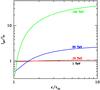 |
Fig. A.1 Ratio of the two integrals IJP(ϵ) and IF(ϵ) as a function of ϵ for ELIV = 1019 GeV and for different values of the γ ray energy, E = 1 TeV (black), 10 TeV (red), 30 TeV (blue) and 100 TeV (green). |
It is possible to check that the two different approaches result in different values of the optical depth. In particular, the Fairbairn et al. treatment provides smaller optical depths for energies above the onset of LIV effects. This can be seen by recasting Eq. (A.1), as used by JP, in the same form of Eq. (A.5), then making the formal change of variable 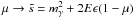 (we note that we are not attributing any physical meaning to this quantity), while maintaining Eq. (A.4) for the argument of σγγ. By doing so, we obtain
 ![Mathematical equation: \appendix \setcounter{section}{1} \begin{eqnarray} \tau_{\rm JP}(E)&=&\int_{0}^{d_{\rm s}} \int _{\epsilon_{\rm min}} \frac{n(\epsilon)}{8E^2\epsilon^2}\int _{\tilde{s}_{\rm min}}^{\tilde{s}_{\rm max}} (\tilde{s}-m^2_{\rm \gamma}) \, \sigma_{\gamma\gamma}(\beta_{\rm JP}) \,{\rm d}\tilde{s} \, {\rm d}\epsilon \, {\rm d}l \nonumber \\[2mm] &=& \int_{0}^{d_{\rm s}} \int _{\epsilon_{\rm min}} \frac{n(\epsilon)}{8E^2\epsilon^2}\, I_{\rm JP}(\epsilon) \, {\rm d}\epsilon \, {\rm d}l \label{tauappjp}, \end{eqnarray}](/articles/aa/full_html/2016/01/aa26071-15/aa26071-15-eq115.png) (A.6)where, using Eq. (2) for ϵmin to expand Eq. (A.4),
(A.6)where, using Eq. (2) for ϵmin to expand Eq. (A.4), ![Mathematical equation: \appendix \setcounter{section}{1} \begin{equation} \beta_{\rm JP}(\tilde{s}) = \left[1 - \frac{\epsilon_{\rm min}}{\epsilon} \right]^{1/2} = \left[1 - \frac{4m_{\rm e}^2c^4-m_{\gamma}^2}{\tilde{s}-m^2_{\gamma}} \right]^{1/2}\cdot \end{equation}](/articles/aa/full_html/2016/01/aa26071-15/aa26071-15-eq116.png) (A.7)Clearly βJP ≠ βF (Eq. (A.3)), determining a different value of the third integrals in Eq. (A.5) and Eq. (A.6), IF(ϵ) and IJP(ϵ).
(A.7)Clearly βJP ≠ βF (Eq. (A.3)), determining a different value of the third integrals in Eq. (A.5) and Eq. (A.6), IF(ϵ) and IJP(ϵ).
The ratio of the two functions IF(ϵ) and IJP(ϵ) for different values of E and ELIV = 1019 GeV appear in Fig. A.1. For energies above the onset of LIV effects IJP(ϵ) >IF(ϵ) for any ϵ (except for a small range around ϵ ~ ϵth), resulting in τJP(E) <τF(E).
Recently, Kifune (2014) stressed the fact that LIV effects can also influence the formation of showers in the atmosphere through which TeV photons are detected.
In fact, we neglect possible LIV terms for electrons.
Acknowledgments
We thank A. Giuliani for input into discussions. We thank the referee for an insightful review that helped us to improve the paper significantly. This work has been partly founded by a PRIN-INAF 2014 grant. The authors acknowledge joint financial support by the CaRiPLo Foundation and the Regional Government of Lombardia for the project ID 2014-1980 “Science and technology at the frontiers of γ-ray astronomy with imaging atmospheric Cherenkov Telescopes”.
References
- Abdo, A. A., Ackermann, M., Ajello, M., et al. 2011, ApJ, 727, 129 [NASA ADS] [CrossRef] [Google Scholar]
- Abeysekara, A. U., Alfaro, R., Alvarez, C., et al. 2013, Astropart. Phys., 50, 26 [NASA ADS] [CrossRef] [Google Scholar]
- Acciari, V. A., Arlen, T., Aune, T., et al. 2011, ApJ, 729, 2 [NASA ADS] [CrossRef] [Google Scholar]
- Acharya, B. S., Actis, M., Aghajani, T., et al. 2013, Astropart. Phys., 43, 3 [Google Scholar]
- Aharonian, F. A., Akhperjanian, A. G., Barrio, J. A., et al. 1999, A&A, 349, 11 [NASA ADS] [Google Scholar]
- Aharonian, F., Akhperjanian, A. G., Barres de Almeida, U., et al. 2007, A&A, 475, L9 [NASA ADS] [CrossRef] [EDP Sciences] [Google Scholar]
- Aliu, E., Archambault, S., Arlen, T., et al. 2014, ApJ, 782, 13 [Google Scholar]
- Amelino-Camelia, G., Ellis, J., Mavromatos, N. E., Nanopoulos, D. V., & Sarkar, S. 1998, Nature, 395, 525 [NASA ADS] [CrossRef] [Google Scholar]
- Amelino-Camelia, G., Mandanici, G., Procaccini, A., & Kowalski-Glikman, J. 2005, Int. J. Mod. Phys. A, 20, 6007 [NASA ADS] [CrossRef] [Google Scholar]
- Bartoli, B., Bernardini, P., Bi, X. J., et al. 2012, ApJ, 758, 2 [NASA ADS] [CrossRef] [Google Scholar]
- Bednarek, W., & Wagner, R. M. 2008, A&A, 486, 679 [NASA ADS] [CrossRef] [EDP Sciences] [Google Scholar]
- Bernlöhr, K., Barnacka, A., Becherini, Y., et al. 2013, Astropart. Phys., 43, 171 [NASA ADS] [CrossRef] [Google Scholar]
- Biteau, J., & Williams, D. A. 2015, ApJ, 812, 60 [NASA ADS] [CrossRef] [Google Scholar]
- Bonnoli, G., Tavecchio, F., Ghisellini, G., & Sbarrato, T. 2015, MNRAS, 451, 611 [NASA ADS] [CrossRef] [Google Scholar]
- Coleman, S., & Glashow, S. L. 1999, Phys. Rev. D, 59, 116008 [NASA ADS] [CrossRef] [Google Scholar]
- Colladay, D., & Kostelecký, V. A. 2001, Phys. Lett. B, 511, 209 [NASA ADS] [CrossRef] [Google Scholar]
- Costamante, L., Ghisellini, G., Giommi, P., et al. 2001, A&A, 371, 512 [NASA ADS] [CrossRef] [EDP Sciences] [Google Scholar]
- Cui, S., Liu, Y., Liu, Y., & Ma, X. 2014, Astropart. Phys., 54, 86 [NASA ADS] [CrossRef] [Google Scholar]
- de Angelis, A., Galanti, G., & Roncadelli, M. 2011, Phys. Rev. D, 84, 105030 [NASA ADS] [CrossRef] [Google Scholar]
- Di Pierro, F., Bigongiari, C., Morello, C., et al. 2013, ArXiv e-prints [arXiv:1307.3992] [Google Scholar]
- Domínguez, A., Primack, J. R., Rosario, D. J., et al. 2011, MNRAS, 410, 2556 [NASA ADS] [CrossRef] [Google Scholar]
- Dwek, E., & Krennrich, F. 2013, Astropart. Phys., 43, 112 [NASA ADS] [CrossRef] [Google Scholar]
- Ellis, J., & Mavromatos, N. E. 2013, Astropart. Phys., 43, 50 [NASA ADS] [CrossRef] [Google Scholar]
- Essey, W., Kalashev, O., Kusenko, A., & Beacom, J. F. 2011, ApJ, 731, 51 [NASA ADS] [CrossRef] [Google Scholar]
- Fairbairn, M., Nilsson, A., Ellis, J., Hinton, J., & White, R. 2014, J. Cosmol. Astropart. Phys., 6, 005 [Google Scholar]
- Jacob, U., & Piran, T. 2008, Phys. Rev. D, 78, 124010 [NASA ADS] [CrossRef] [Google Scholar]
- Jacob, U., Mercati, F., Amelino-Camelia, G., & Piran, T. 2010, Phys. Rev. D, 82, 084021 [NASA ADS] [CrossRef] [Google Scholar]
- Jacobson, T., Liberati, S., & Mattingly, D. 2003, Phys. Rev. D, 67, 124011 [NASA ADS] [CrossRef] [Google Scholar]
- Katarzyński, K., Ghisellini, G., Tavecchio, F., Gracia, J., & Maraschi, L. 2006, MNRAS, 368, L52 [NASA ADS] [CrossRef] [Google Scholar]
- Kaufmann, S., Wagner, S. J., Tibolla, O., & Hauser, M. 2011, A&A, 534, A130 [NASA ADS] [CrossRef] [EDP Sciences] [Google Scholar]
- Kifune, T. 1999, ApJ, 518, L21 [NASA ADS] [CrossRef] [Google Scholar]
- Kifune, T. 2014, ApJ, 787, 4 [NASA ADS] [CrossRef] [Google Scholar]
- Lefa, E., Rieger, F. M., & Aharonian, F. 2011, ApJ, 740, 64 [NASA ADS] [CrossRef] [Google Scholar]
- Liberati, S. 2013, Class. Quant. Grav., 30, 133001 [NASA ADS] [CrossRef] [Google Scholar]
- Mattingly, D. 2005, Liv. Rev. Relat., 8, 5 [Google Scholar]
- Murase, K., Dermer, C. D., Takami, H., & Migliori, G. 2012, ApJ, 749, 63 [Google Scholar]
- Neronov, A., Semikoz, D., & Taylor, A. M. 2012, A&A, 541, A31 [NASA ADS] [CrossRef] [EDP Sciences] [Google Scholar]
- Protheroe, R. J., & Meyer, H. 2000, Phys. Lett. B, 493, 1 [NASA ADS] [CrossRef] [Google Scholar]
- Rubtsov, G., Satunin, P., & Sibiryakov, S. 2012, Phys. Rev. D, 86, 085012 [NASA ADS] [CrossRef] [Google Scholar]
- Tavecchio, F., Ghisellini, G., Ghirlanda, G., Costamante, L., & Franceschini, A. 2009, MNRAS, 399, L59 [NASA ADS] [CrossRef] [Google Scholar]
- Tavecchio, F., Ghisellini, G., Bonnoli, G., & Foschini, L. 2011, MNRAS, 414, 3566 [NASA ADS] [CrossRef] [Google Scholar]
- Tluczykont, M., Hampf, D., Horns, D., et al. 2014, Astropart. Phys., 56, 42 [NASA ADS] [CrossRef] [Google Scholar]
- Vasileiou, V., Jacholkowska, A., Piron, F., et al. 2013, Phys. Rev. D, 87, 122001 [NASA ADS] [CrossRef] [Google Scholar]
- Vercellone, S., Agnetta, G., Antonelli, L. A., et al. 2013, ArXiv e-prints [arXiv:1307.5671] [Google Scholar]
- Zacharopoulou, O., Khangulyan, D., Aharonian, F. A., & Costamante, L. 2011, ApJ, 738, 157 [NASA ADS] [CrossRef] [Google Scholar]
All Figures
|
Fig. 1 Left: photon target energy at threshold ϵmin for the pair-production reaction as a function of the γ-ray energy Eγ. The black solid line shows the standard case. The other lines indicate the modified threshold, which result from the LIV-modified kinematics, for different values of the parameter ELIV (in units of 1019 GeV). Right: EBL (Dominguez et al. 2011, solid red; Kneiske & Dole 2010, solid blue) and CMB (dashed red) local density ϵn(ϵ) (horizontal axis) as a function of the energy ϵ (vertical axis), to be compared with the energy threshold in the left panel. |
| In the text | |
|
Fig. 2 Absorption coefficient e− τγγ as a function of energy for γ rays that propagate from a source at z = 0.03 (upper panel) and z = 0.14 (lower panel), using the EBL model of Dominguez et al. (2011). The black solid line indicates the standard case, the other lines show the modified coefficient for different values of ELIV (with the color code reported in the caption). Thick lines have been obtained using the treatment of Fairbairn et al. (2014). For comparison, thin lines show the results of the calculations that were based on the assumptions of Jacob & Piran (2008). |
| In the text | |
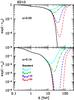 |
Fig. 3 As Fig. 2, but using the EBL model of Kneiske & Dole (2010). |
| In the text | |
|
Fig. 4 Observed γ-ray spectrum of Mkn 501 during the 1997 active state recorded HEGRA (red symbols). The black solid and dotted orange lines show the observed and the intrinsic spectrum, assuming standard absorption with the D11 (upper panel) and KD10 (lower panel) EBL models. Grey points indicate the observed data points corrected for absorption. Other lines show the predicted spectrum with LIV effects (line styles and colors as in Fig. 2). The violet lines show the 5σ sensitivity curves for CTA (5 h, dashed and 50 h exposure, solid). |
| In the text | |
|
Fig. 5 Observed γ-ray spectrum of Mkn 501 during a quiescent phase (Acciari et al. 2011). The three panels report the received γ-ray spectrum for different assumed intrinsic spectra (from top to bottom: a simple power law with energy index α = 0.52; a power law with energy index α = 0.52 and an exponential cut-off with e-folding energy Ecut = 50 TeV; a cut-offed power law with α = 0.52 and Ecut = 15 TeV) and values of ELIV (color code as in Fig. 2). The HAWC and CTA sensitivity curves (as in Fig. 3) are displayed for an exposure time of one year and 50 h, respectively. |
| In the text | |
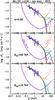 |
Fig. 6 As Fig. 5 but with the KD10 EBL model. |
| In the text | |
|
Fig. 7 Observed high-energy SED of 1ES 0229+200. Black symbols are LAT measurements from the 3FGL catalogue. Orange triangles indicate the HESS spectrum (Aharonian et al. 2007) while the gray triangles indicate fluxes that are obtained after correction for the absorption with EBL. The dotted line indicates the assumed intrinsic spectrum. The three panels report the received γ-ray spectrum for different assumed intrinsic spectra (from top to bottom: a simple power law with energy index α = 0.4; a broken power law with high-energy index α2 = 2 and break energy Eb = 10 TeV; an exponential cut-off with e-folding energy Ecut = 15 TeV) and values of ELIV (color code as in Fig. 2). The HAWC and CTA sensitivity curves (as in Fig. 3) are displayed for an exposure time of five years and 50 h, respectively. |
| In the text | |
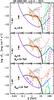 |
Fig. 8 As Fig. 7, but with the KD10 EBL model and α = 0.5. |
| In the text | |
|
Fig. A.1 Ratio of the two integrals IJP(ϵ) and IF(ϵ) as a function of ϵ for ELIV = 1019 GeV and for different values of the γ ray energy, E = 1 TeV (black), 10 TeV (red), 30 TeV (blue) and 100 TeV (green). |
| In the text | |
Current usage metrics show cumulative count of Article Views (full-text article views including HTML views, PDF and ePub downloads, according to the available data) and Abstracts Views on Vision4Press platform.
Data correspond to usage on the plateform after 2015. The current usage metrics is available 48-96 hours after online publication and is updated daily on week days.
Initial download of the metrics may take a while.