© ESO, 2015

1. Introduction

Many eruptive phenomena on the Sun, such as solar flares and coronal mass ejections (CMEs), are accompanied by outbursts of energetic charged particles known as solar energetic particle (SEP) events. The events associated with CMEs are thought to be produced by shock waves driven by ejections moving rapidly through solar wind plasma. The main acceleration mechanism of ions at these kinds of shocks is considered to be diffusive shock acceleration (DSA, Axford et al. 1977; Krymskii 1977; Blandford & Ostriker 1978; Bell 1978), in which particles get energized by repeatedly crossing the shock. In the case of quasi-parallel shocks, an essential role in the mechanism is given to the Alfvénic turbulence in the vicinity of the shock, which scatters particles in pitch angle and facilitates the return of particles back to the shock. On the other hand, efficient operation of DSA requires the turbulence ahead of the shock, i.e. in the foreshock, to be much stronger than that expected in the ambient corona/interplanetary space. This is achieved by means of the accelerated particles themselves, which generate Alfvén waves due to a streaming instability (Bell 1978). This couples the processes of particle acceleration and turbulence evolution.

There are a number of analytical theories of particle acceleration at shocks, accounting for the particle-wave coupling (Bell 1978; Lee 1983, 2005; Gordon et al. 1999), which, however, rely on the assumption of a steady state for particles and waves. In other words, even if the shock parameters change with time, e.g. because of the shock propagation away from the Sun, the particle/wave distributions represent a temporal sequence of stationary solutions depending on the current shock parameters. In spite of the progress associated with the proposed theories, there has been an interest to take the dynamical behaviour of the system into account. As a result of the complexity of the problem, this has been done with numerical simulations. One of the approaches was suggested by Zank et al. (2000) and further developed in, e.g. Li et al. (2003, 2005). With this approach, the transport of particles in the shock vicinity is treated numerically, but the accelerated particle spectrum at the shock is approximated analytically. Further development has been pointed towards a completely self-consistent dynamic modelling of particle acceleration (for the results, see e.g. Vainio & Laitinen 2007, 2008; Ng & Reames 2008; Battarbee et al. 2011; Battarbee 2013; Vainio et al. 2014).

Self-consistent Monte Carlo simulations are one of the approaches in constructing dynamical models of particle acceleration. Since these simulations are based on the consideration of individual particles interacting with turbulence, they can provide detailed information on particle and turbulence distributions in the vicinity of the shock. Current Monte Carlo simulations use the quasi-linear theory (Jokipii 1966) applicable for interactions of particles with weak slab-mode turbulence (represented by e.g. the spectrum of low-amplitude Alfvén waves). In quasi-linear theory, wave-particle interactions are resonant and governed by the following resonance condition (written in the wave rest frame): ${\mathit{k}}_{\mathrm{res}}\mathrm{=}\frac{\mathrm{\Omega }}{\mathit{\upsilon \mu }}\mathit{,}$(1)where k_res is the (resonant) wavenumber, υ and μ are the particle speed and pitch-angle cosine as measured in the wave rest frame, Ω = γ^-1Ω₀, Ω₀ is the particle cyclotron frequency and γ is the relativistic factor. Furthermore, particle pitch-angle scattering is determined by the pitch-angle diffusion coefficient 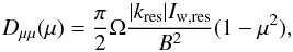${\mathit{D}}_{\mathit{\mu \mu }}\mathrm{\left(}\mathit{\mu }\mathrm{\right)}\mathrm{=}\frac{\mathit{\pi }}{\mathrm{2}}\mathrm{\Omega }\frac{\mathrm{\left|}{\mathit{k}}_{\mathrm{res}}\mathrm{\right|}{\mathit{I}}_{\mathrm{w}\mathit{,}\mathrm{res}}}{{\mathit{B}}^{\mathrm{2}}}\mathrm{(}\mathrm{1}\mathrm{-}{\mathit{\mu }}^{\mathrm{2}}\mathrm{)}\mathit{,}$(2)where B is the mean magnetic field and I_w,res is the value of the wave intensity spectrum I_w(k) at k = k_res.

In recent years, the Coronal Shock Acceleration (CSA) Monte Carlo code (Vainio & Laitinen 2007, 2008; Battarbee et al. 2011; Battarbee 2013) has been extensively used to study particle acceleration and foreshock evolution in coronal shocks. The advantage of the code is that it allows for simulations of acceleration in parallel or oblique shocks on a global spatial scale (the shock can cover a distance of tens of solar radii in a single simulation). However, its performance is largely achieved via a simplified pitch-angle resonance condition, ${\mathit{k}}_{\mathrm{res}}\mathrm{=}\frac{\mathrm{\Omega }}{\mathit{\upsilon }}\mathit{,}$(3)which leads to isotropic pitch-angle scattering 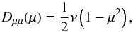${\mathit{D}}_{\mathit{\mu \mu }}\mathrm{\left(}\mathit{\mu }\mathrm{\right)}\mathrm{=}\frac{\mathrm{1}}{\mathrm{2}}\mathit{\nu }\mathrm{(}\mathrm{1}\mathrm{-}{\mathit{\mu }}^{\mathrm{2}}\mathrm{)}\mathit{,}$(4)where the particle scattering rate ν = πΩ²I_w,res/ (υB²) does not depend on the pitch angle. The simplified resonance condition implies that particles at a particular speed interact with only one particular spectral component of the wave intensity spectrum. Moreover, Eq. (4) shows that the resonance gap does not appear (instead, the pitch-angle diffusion coefficient has a maximum at μ = 0). Although it is generally accepted that quasi-linear theory does not work close to μ = 0 (see e.g. introduction in Ng & Reames 1995 and references therein) and particle acceleration and transport simulation studies usually employ so-called filling of the resonance gap, one can suspect an over-efficiency of particle acceleration in CSA simulations. Also, the ability of particles to interact with multiple wave spectral components creates new effects that are not reproduced if the simplified pitch-angle scattering model is used (Ng & Reames 2008).

To study the effect of anisotropic pitch-angle scattering on particles acceleration at coronal shocks, we developed a new Monte Carlo code named SOLar Particle Acceleration in Coronal Shocks (SOLPACS). Contrary to the CSA code, this code utilizes the full quasi-linear resonance condition of pitch-angle scattering (Afanasiev & Vainio 2013). In the present paper, we compare SOLPACS simulation results with those of CSA, obtained for the same initial and boundary conditions, and with the steady-state theory of diffusive shock acceleration (Bell 1978, see also Vainio & Laitinen 2007, 2008 and Vainio et al. 2014).

Further, in Sect. 2, we review some aspects of the steady-state theory, which are further used in the analysis of the simulations. In Sect. 3, we describe the simulation set-up. In Sect. 4, we present simulation results and their comparative analysis. In Sect. 5, we provide further discussion of SOLPACS and CSA results. Finally, in Sect. 6, we present our conclusions.

2. Steady-state theory

Here we specify the accelerated particles by the conventional distribution function f = d⁶N/ (dx³ dp³) in phase space, and Alfvén waves by the wave intensity I_w, which is defined by 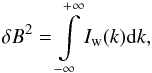$\mathit{\delta }{\mathit{B}}^{\mathrm{2}}\mathrm{=}\underset{\mathrm{-}\mathrm{\infty }}{\overset{\mathrm{+}\mathrm{\infty }}{\mathrm{\int }}}{\mathit{I}}_{\mathrm{w}}\mathrm{\left(}\mathit{k}\mathrm{\right)}\mathrm{d}\mathit{k,}$(5)where the positive and negative values of k correspond to the waves with opposite circular polarizations. Then, Bell’s steady-state theory of diffusive shock acceleration at a (planar) parallel shock can be presented in the following form (Vainio & Laitinen 2007; Vainio et al. 2014): 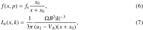$\begin{array}{ccc}& & \\ & & \end{array}$where

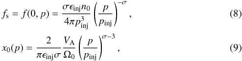$\begin{array}{ccc}& & \\ & & \end{array}$xis the distance from the shock towards the upstream region along the mean magnetic field; u₁ is the shock-frame solar wind speed; V_A is the Alfvén speed; n₀ is the thermal proton density in the shock’s upstream; σ = 3r_c/ (r_c−1) is the spectral index of the particle distribution function at shock; r_c = V₁/V₂ is the scattering-centre compression ratio, which is defined as the ratio of the shock-frame phase velocities V₁ and V₂ of Alfvén wave modes in the upstream and downstream regions, respectively (see, Vainio & Schlickeiser 1998 for details); and ϵ_inj is the fraction of upstream protons injected into the acceleration process at the injection momentum, p_inj. The parameter x₀(p) in Eq. (9) has to be expressed as a function of k, before it can be substituted to Eq. (7), applying the resonance condition, p = m_pΩ₀/ | k |. The parameter ϵ_inj is related to the particle injection rate Q (the number of particles injected at the shock per unit cross-section of the shock and unit time) through Q = ϵ_injn₀u₁, where n₀ is the thermal proton density in the shock’s upstream. The parameter p_inj can be calculated from (Vainio & Laitinen 2007) 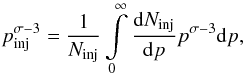${\mathit{p}}_{\mathrm{inj}}^{\mathit{\sigma }\mathrm{-}\mathrm{3}}\mathrm{=}\frac{\mathrm{1}}{{\mathit{N}}_{\mathrm{inj}}}\underset{\mathrm{0}}{\overset{\mathrm{\infty }}{\mathrm{\int }}}\frac{\mathrm{d}{\mathit{N}}_{\mathrm{inj}}}{\mathrm{d}\mathit{p}}{\mathit{p}}^{\mathit{\sigma }\mathrm{-}\mathrm{3}}\mathrm{d}\mathit{p,}$(10)where dN_inj/ dp is the injected particle spectrum.

Using Eqs. (6) and (8), one can calculate the omni-directional particle intensity I(x,p) = p²f(x,p) and, using energy E as an independent variable, obtain at the shock (in the non-relativistic regime): I(E) ∝ E^{1−σ/ 2}. Considering the wave intensity I_w(x,k), it is easy to see from Eq. (9) that x₀(k) ∝ | k | ^3−σ (σ> 3). At a given distance x from the shock, defining k_b as the solution of x₀(k) = x, Eq. (7) reveals that the wave intensity represents a broken power law in k: at | k | ≫ k_b, we obtain I_w(k) ∝ | k | ^-3, and at | k | ≪ k_b, we get I_w(k) ∝ | k | ^σ−6. The break point k_b decreases with distance from the shock.

Additionally, one can calculate the particle mean free path λ, which is defined as 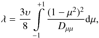$\mathit{\lambda }\mathrm{=}\frac{\mathrm{3}\mathit{\upsilon }}{\mathrm{8}}\underset{-1}{\overset{\mathrm{+}\mathrm{1}}{\mathrm{\int }}}\frac{\mathrm{(}\mathrm{1}\mathrm{-}{\mathit{\mu }}^{\mathrm{2}}{\mathrm{)}}^{\mathrm{2}}}{{\mathit{D}}_{\mathit{\mu \mu }}}\mathrm{d}\mathit{\mu ,}$(11)but in Bell’s steady-state DSA theory, after applying the simplified resonance condition, it reads (Vainio et al. 2014) $\mathit{\lambda }\mathrm{\left(}\mathit{x,\upsilon }\mathrm{\right)}\mathrm{=}\frac{\mathrm{3}\mathrm{(}{\mathit{u}}_{\mathrm{1}}\mathrm{-}{\mathit{V}}_{\mathrm{A}}\mathrm{)}}{\mathit{\upsilon }}\mathrm{(}\mathit{x}\mathrm{+}{\mathit{x}}_{\mathrm{0}}\mathrm{)}\mathit{.}$(12)Finally, one can estimate the cut-off energy in the particle energy spectrum, I(E), which can occur because of, e.g. a finite acceleration time, using the mean free path resulting from Bell’s steady-state theory. In that case, assuming a parallel shock and constant parameters specifying the shock and plasma (which is the case in our simulations), one can obtain an estimate for the cut-off momentum p_c for the shock propagating in time t_s (Vainio et al. 2014), i.e. ${\mathit{p}}_{\mathrm{c}}^{\mathit{\sigma }\mathrm{-}\mathrm{3}}\mathrm{=}{\mathit{p}}_{\mathrm{inj}}^{\mathit{\sigma }\mathrm{-}\mathrm{3}}\left(\mathrm{1}\mathrm{+}\frac{\mathit{\pi }}{\mathrm{2}}\frac{{\mathit{ϵ}}_{\mathrm{inj}}\mathit{\sigma }\mathrm{(}{\mathit{M}}_{\mathrm{A}}\mathrm{-}\mathrm{1}\mathrm{)}}{{\mathit{r}}_{\mathrm{c}}}{\mathrm{\Omega }}_{\mathrm{0}}{\mathit{t}}_{\mathrm{s}}\right)\mathit{,}$(13)where M_A = u₁/V_A is the Alvénic Mach number of the upstream flow.

3. Simulation set-up

In both CSA and SOLPACS, particles are traced within a 1D spatial simulation box, i.e. along the mean magnetic field line. Although CSA allows variation of the plasma density and magnetic field with distance from the Sun, here we focus on effects produced by the two different wave-particle interaction models. Therefore, we perform simulations for a simple set-up, assuming constant thermal proton density, n₀ = 3.6 × 10¹² m^-3, magnetic field, B₀ = 3.4 × 10^-5 T and solar wind speed, u₀ = 12.4km s^-1 in the whole simulation domain. The applied values correspond to the density, magnetic field, and solar wind speed given by the coronal model of Vainio & Laitinen (2007) for the heliocentric distance of 2 R_⊙. The implied locality of the simulations allows us to consider the simulation box to be moving with the shock, i.e. in the shock frame. In this case, simulating only the upstream region, we take the shock itself as one boundary of the box. The other boundary is taken to be at a distance of 1 R_⊙ from the shock. Further, we assume the plasma turbulence in the box to be due to outwards-propagating (if considered in the solar wind frame) Alfvén waves, with the initial spectral form ∝ k^{− 3/2}. We select a low initial wave intensity, such that it provides little pitch-angle scattering for injected particles, i.e. a non-diffusive particle transport, in the spatial simulation box at early times in a simulation. Specifically, it is calculated assuming the initial mean free path λ = 1 R_⊙ for 100 keV protons in both CSA and SOLPACS¹. We simulate protons, which are assumed to be injected at the shock at a constant rate Q, which is characterized by the injection efficiency ϵ_inj. Similar to Vainio & Laitinen (2007), the injected particles are characterized by an exponential velocity spectrum (in the shock frame) dN_inj/ dυ = (N_inj/υ₁)H(υ−u₁)e^{− (υ−u₁) /υ₁}, where N_inj = Qt is the number of particles per unit cross-section of the magnetic flux tube injected in time t, υ₁ is a parameter, and H is the Heaviside step function. Similar to Vainio & Laitinen (2007), instead of tracing particles in the shock’s downstream, we employ a probability of return from the downstream (Jones & Ellison 1991), P_ret = (υ_w−V₂)²/ (υ_w + V₂)², where υ_w is the particle speed in the frame of the downstream waves and V₂ = (u₁−V_A) /r_c is the effective speed of dowstream Alfvén waves as measured in the shock frame. In our simulations, we take the shock speed V_s = 1500 km s^-1 and fix the scattering-centre compression ratio to r_c = 4 and υ₁ = 375 km s^-1. For the assumed values, from Eq. (10) we obtain p_inj = m_p(u₁ + υ₁), which gives ${\mathit{E}}_{\mathrm{inj}}\mathrm{=}{\mathit{p}}_{\mathrm{inj}}^{\mathrm{2}}\mathit{/}\mathrm{\left(}\mathrm{2}{\mathit{m}}_{\mathrm{p}}\mathrm{\right)}\mathrm{=}\mathrm{18.1}\hspace{0.17em}\mathrm{keV}$.

The numerical scheme to simulate wave-particle interactions, implemented in SOLPACS, is detailed in Afanasiev & Vainio (2013). In the following, we recall two main points important for the analysis of simulation data.

At each time step in a simulation, the wave intensity spectrum I_w(k) is given by its values at the k-grid nodes { k_j } and by a set of spectral indices { q_j } resulting from interpolation of those values by a power-law function between every two adjacent k-grid nodes: q_j = ln(I_{w,j + 1}/I_w,j)/ln(k_{j + 1}/k_j). Therefore, for k ∈ (k_j,k_{j + 1}), we have I_w(k) = I_w,j(k/k_j)^{− q_j}. Considering the μ-grid: { μ_j = Ω/(υk_j) }, for μ ∈ (μ_{j + 1},μ_j), we obtain ν(μ) = ν_0,j | μ | ^q_j−1, where ν_0,j = πΩ /B²(υ/ Ω)^q_j−1I_w,j | k_j | ^q_j. Using this notation, the mean free path (Eq. (11)) can be calculated as $\mathit{\lambda }\mathrm{=}\frac{\mathrm{3}\mathit{\upsilon }}{\mathrm{4}}\sum _{\mathit{j}}{\mathrm{\int }}_{{\mathit{\mu }}_{\mathit{j}\mathrm{+}\mathrm{1}}}^{{\mathit{\mu }}_{\mathit{j}}}\frac{\mathrm{1}\mathrm{-}{\mathit{\mu }}^{\mathrm{2}}}{{\mathit{\nu }}_{\mathrm{0}\mathit{,j}}\mathrm{|}\mathit{\mu }{\mathrm{|}}^{{\mathit{q}}_{\mathit{j}}\mathrm{-}\mathrm{1}}}\mathrm{d}\mathit{\mu ,}$(14)where summation is performed over the grid nodes in μ-space.

The employed pitch-angle scattering method requires extremely small time steps to be taken near μ = 0. Therefore, we fill the resonance gap by approximating the scattering frequency ν(μ) near μ = 0 by a linear function $\begin{array}{c}{}^{\mathrm{􏽥}}\\ \mathit{\nu }\end{array}\mathrm{\left(}\mathit{\mu }\mathrm{\right)}\mathrm{=}\mathit{b\mu }\mathrm{+}{\mathit{b}}_{\mathrm{1}}$ in the interval (− μ_min,μ_min), where μ_min = Ω/(υk_max) and k_max is the maximum node of the k-grid, which is taken to be about Ω₀/V_A. In these simulations, k_max = 10^-2 m^-1. The technique applied makes the resonance gap in the μ-space narrower for higher-energy particles than for low-energy particles.

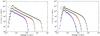Fig. 1 Simulated particle energy spectra obtained with CSA (left panel) and SOLPACS (right panel) at t = 580 s for different values of the injection efficiency: ϵinj = 1.62 × 10-6 (blue circles), ϵinj = 5.40 × 10-6 (red circles), and ϵinj = 1.62 × 10-5 (green circles). Black curves represent fits to the spectral data, obtained with Eq. (15). The fitting was carried out at energies E> 0.2 MeV in all cases.

4. Results

We have carried out simulations for three different values of the particle injection rate at the shock (given by the parameter ϵ_inj). The simulations were conducted until the time in a simulation reached t_max = 580 s, which corresponds to the shock propagation distance of 1.25 R_⊙. Figure 1 presents resulting proton energy spectra, I(E), at the shock at t = t_max. The presented spectra are calculated in the solar-fixed frame (where the shock propagates at speed V_s). Similar to Vainio et al. (2014), we fitted the spectral data by the function $\mathit{I}\mathrm{\left(}\mathit{E}\mathrm{\right)}\mathrm{=}\mathit{C}{\mathit{E}}^{\mathrm{-}\mathit{\beta }}\exp \begin{array}{c}\mathrm{⎧}\\ \mathrm{⎪}\\ \mathrm{⎪}\\ \mathrm{⎨}\\ \mathrm{⎪}\\ \mathrm{⎪}\\ \mathrm{⎩}\end{array}\mathrm{-}{\left(\frac{\mathit{E}}{{\mathit{E}}_{\mathrm{c}}}\right)}^{\mathit{\delta }}\begin{array}{c}\mathrm{⎫}\\ \mathrm{⎪}\\ \mathrm{⎪}\\ \mathrm{⎬}\\ \mathrm{⎪}\\ \mathrm{⎪}\\ \mathrm{⎭}\end{array}\mathit{,}$(15)where C, β, E_c, and δ are fitting parameters. The fits are shown in Fig. 1 as well. The best-fit values of the spectral parameters along with the errors are given in Table 1. The indicated errors account for statistical errors in the spectral data and systematic errors due to binning of the data and the non-power-law form of the spectra at low energies (visible as quasi-regular variations of the particle intensity on the plots). In order to avoid large systematic errors caused by such variations, the spectra were fitted at E> 0.2 MeV. The details of the fitting algorithm and of the error calculations are given in Appendix A. When fitting the spectra corresponding to the weakest injection ($\mathit{ϵ}{\mathrm{inj}}_{}\mathrm{=}\mathrm{1.62}\mathrm{\times }{\mathrm{10}}^{-6}$), the power-law index β was fixed to 1 (the theoretical value) as the power-law-like portion of the spectrum to be fitted was quite small (not recognizable at all in the case of the SOLPACS simulation). The spectra have similar shapes consisting of a low-energy, multi-peak component, a power-law part, and a super-exponential tail in all cases, although the spectra corresponding to anisotropic pitch-angle scattering have smaller values of the cut-off energy E_c and the cut-off steepness δ.

Figure 2 presents spatial distributions of particles of different energies in the foreshock, resulting from CSA and SOLPACS in comparison with those resulting from Bell’s steady-state theory. The plotted distributions are calculated in the mixed reference frame, i.e. the particle intensity I(x,p′) represents a function of the distance x, as measured in the shock frame, and of the momentum p′, as measured in the solar fixed frame. We apply a correction to the theoretical distributions by multiplying the injection efficiency ϵ_inj (Eqs. (8) and (9)) by a factor α, where 1 <α< 2, which accounts for the difference in the pitch-angle distribution of injected particles in Bell’s theory and in our simulations. Bell’s theory injects particles isotropically, whereas our simulations only inject into one hemisphere (μ> 0) (Vainio & Laitinen 2008). We find that α = 1.8 gives the best correspondence between the CSA distributions and the theoretical distributions in the vicinity of the shock. Their deviation, increasing with distance, is due to the free escape of particles at the outer boundary of the simulation box. In the case of SOLPACS, the behaviour of particles in the foreshock is much more complicated than predicted by Bell’s steady-state theory. In very close vicinity of the shock (x ≲ 5 × 10^-3R_⊙), the energy dependence of the particle intensity is similar for both simulations and theory. However, that is not the case further in the foreshock. The most dramatic difference is experienced by low-energy particles: there is a region in the foreshock, in which there is a lack of these particles in comparison with the theoretical prediction. And on the contrary, particles of higher energies are in excess compared to the theory in the whole foreshock region.

To get more information, we looked at the time evolution of spatial distributions of particles, produced by SOLPACS, at two energies, 0.1 MeV and 1 MeV (Fig. 3). One can see, in the case of low energy, the particle intensity first increases with time (at a given location in the foreshock), reaches a maximum, and then decreases at a much slower rate. In the case of high-energy particles, the time evolution of their spatial profile is different: the particle intensity increases with time and largely stagnates close to its maximum level. There is also a flattening before the steep tail in the spatial profiles of 0.1 MeV particles.

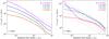Fig. 2 Distribution of particles in the foreshock at different energies, resulting from CSA (left panel, continuous curves) and SOLPACS (right panel, continuous curves) at the end (t = 580 s) of the simulation for ϵinj = 1.62 × 10-5 compared to Bell’s steady-state theory (dashed curves).

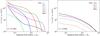Fig. 3 Time evolution of the spatial distribution of particles in the foreshock at E = 0.1 MeV (left panel) and E = 1.0 MeV (right panel) in SOLPACS. Dashed red and green curves in the right panel correspond to additional times t = 195 s and 235s.

Figure 4 shows Alfvén wave spectra at the end (t = 580 s) of the simulations for ϵ_inj = 1.62 × 10^-5 in close vicinity of the shock and at some distance in the foreshock. One can see, first of all, that the spectra resulting from the CSA simulation are more intense at lower wavenumbers than the SOLPACS spectra. Moreover, the wave generation in the CSA simulation reaches smaller wavenumbers than in the case of the SOLPACS one. This is in agreement with the difference in the cut-off energy E_c in the corresponding particle energy spectra at the shock. Also, in the CSA spectra, the spectrum amplification drops off at k ~ 10^-3 m^-1, whereas in the SOLPACS spectra the amplification extends up to the highest wavenumbers.

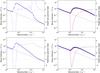Fig. 4 Wave intensity spectra obtained with CSA (left column) and SOLPACS (right column) for ϵinj = 1.62 × 10-5 at distance x = 0.0035 R⊙ (top row) and x = 0.13 R⊙ (bottom row) in front of the shock at t = 580 s. The filled blue and red circles in the SOLPACS data plots denote wave intensities of Alfvén waves of the opposite circular polarization. In all plots, coloured dashed lines show spectral indices and black dashed line shows the initial spectrum, normalized to provide λ = 1 R⊙ for 100 keV protons.

In Fig. 5, we present spatial distributions of the particle mean free path in the foreshock at different energies, calculated from CSA and SOLPACS data along with the mean free paths predicted by Bell’s steady-state theory. To obtain the theoretical mean free path, the same value of the correction factor α = 1.8 is applied. The mean free path resulting from CSA was calculated as λ = υ/ν, which results from Eq. (11) supplemented by Eq. (4), and the mean free path resulting from SOLPACS was calculated with Eq. (14), in which we took the resonance gap filling into account. One can see that the mean free path calculated based on the SOLPACS simulation data increases with energy, whereas the mean free path calculated using the steady-state theory demonstrates the opposite dependence on energy. The mean free path resulting from the CSA simulation data has a more complex behaviour, although this mean free path demonstrates similarity with the steady-state theory prediction close to the shock.

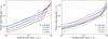Fig. 5 Proton mean free path as a function of distance from the shock, calculated for different energies for ϵinj = 1.62 × 10-5 at t = 580 s. Left panel: CSA (continuous curves) vs. steady-state theory (dashed curves); right panel: SOLPACS (continious curves) vs. steady-state theory (dashed curves).

Figure 6 demonstrates the evolution of the foreshock mean free path with time in CSA and SOLPACS. In CSA the mean free path achieves a steady state but in SOLPACS it does not. The behaviour of the mean free path at higher energies is qualitatively similar to the presented case for E = 0.1 MeV. Figure 7 shows the SOLPACS energy dependence of the mean free path in the vicinity of the shock.

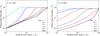Fig. 6 Time evolution of the proton mean free path in the foreshock at E = 0.1 MeV in CSA (left panel) and SOLPACS (right panel) for ϵinj = 1.62 × 10-5.

5. Discussion

The simulations performed demonstrate that anisotropic pitch-angle scattering and the corresponding modification in the wave growth rate lead to less efficient acceleration of particles at a shock. We can compare the acceleration efficiency provided by different models by comparing spectral cut-off energies (Fig. 8, left panel). The theoretical values of the cut-off energy were calculated using Eq. (13). One can see that the anisotropic pitch-angle scattering provides an additional downscaling of the cut-off energy (approximately by a factor of 5) over the CSA result, which is already an order of magnitude lower than that provided by Bell’s steady-state theory. The SOLPACS cut-off energies are well fitted by a power law that one can extrapolate to larger (but still reasonable) values of the injection efficiency. One can see that for ϵ_inj = 5 × 10^-4 our extrapolation yields E_c ≈ 300 MeV. So, particle acceleration with SOLPACS is still efficient in the sense that particles can be accelerated to relativistic energies within ten minutes or less. On the right panel of Fig. 8, we present the values of the cut-off steepness δ obtained in the simulations. We see that SOLPACS provides less abrupt spectral cut-offs compared to CSA, although the spectral form is still somewhat steeper than in observations of large SEP events (see e.g. Tylka & Dietrich 2009; Afanasiev et al. 2014). However, it is difficult to make a reliable prediction for δ at large ϵ_inj, based on the data available from the present simulations. This problem will be addressed in forthcoming work.

The error analysis of the values of the fitted spectral parameters (see Table 1) shows that the power-law index β of the particle spectrum obtained with SOLPACS for ϵ_inj = 1.62 × 10^-5 is about 8% lower than the theoretical index. We speculate that this happens because of ballistic removal of low-energy particles from the shock since it should take a longer time for these sorts of particles to scatter over μ = 0 than for higher-energy particles (the resonance gap is wider for lower-energy particles than for higher-energy particles). The existence of the plateau-like feature in the spatial distributions of low-energy particles and its absence for high-energy particles (Fig. 3) supports this idea. Therefore, the plateau feature represents low-energy particles that propagated to those distances early in the simulation, i.e. when their turbulent trapping was not very efficient. At later times, the trapping becomes efficient and does not allow any new low-energy particles to reach those distances, which is consistent with the large intensity gradient of low-energy protons close to the shock.

The distinctions between the wave spectra resulting from CSA and SOLPACS, shown in Fig. 4, are due to different forms of the resonance condition of pitch-angle scattering employed in the codes. The top row of Fig. 4 shows wave spectra at distance x = 3.5 × 10^-3R_⊙ from the shock. Using Eq. (9) of Bell’s steady-state theory, along with the corresponding resonance condition p = m_pΩ₀/k, we estimate that k_b = 4.20 × 10^-4 m^-1. For the bottom row of plots in Fig. 4, corresponding to x = 0.13 R_⊙, we find k_b = 2.26 × 10^-5 m^-1. For σ = 4, Bell’s theory predicts x₀ ∝ k^-1 and I_w(k) ∝ k^-2 at k ≪ k_b and I_w(k) ∝ k^-3 at k ≫ k_b. One can see that the SOLPACS wave spectra have variable spectral indices q ≲ 2, which thus contradicts Bell’s steady-state theory. By contrast, the CSA spectra (at the wavenumber interval of 10^-4 ≲ k ≲ 10^-3 m^-1, where the bulk of particles is in resonance) have spectral indices q between 2 and 3, and become steeper with distance, in agreement with the steady-state theory. The asymptotic form ~k^-2 of the SOLPACS spectra is consistent with earlier studies of wave generation by anisotropic particle distributions, using the full resonance condition (Lee & Ip 1987; Gordon et al. 1999; Schlickeiser et al. 2002; Afanasiev & Vainio 2013).

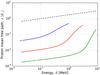Fig. 7 Proton mean free path as a function of energy in the vicinity of the shock obtained with SOLPACS for different values of the injection parameter: ϵinj = 1.62 × 10-6 (blue), ϵinj = 5.40 × 10-6 (red) and ϵinj = 1.62 × 10-5 (green) at t = 580 s. Dashed line corresponds to the mean free path in the background plasma with the wave spectrum Iw ∝ k− 3/2 (λ ∝ E1/4).

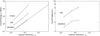Fig. 8 Left panel: cut-off energy Ec versus injection efficiency ϵinj, resulting from the simulations and steady-state theory. Dashed curve represents a power-law extrapolation of SOLPACS results to larger values of ϵinj. Right panel: cut-off steepness δ versus injection efficiency ϵinj, resulting from the simulations.

The shape of the wave spectrum governs the energy dependence of the particle mean free path in the foreshock (Fig. 5). For σ = 4, the steady-state theory (Eq. (12)) gives λ ∝ E^{− 1/2} (non-relativistic regime) at large distances from the shock (x ≫ x₀). When approaching the shock the differences between mean free paths corresponding to different energies reduce and vanish at the shock. In the case of CSA simulations, | k_res | = Ω /υ, I_w,res ∝ | k_res | ^{− q}. Therefore, λ = υ/ν ∝ E^{− (q/ 2−1)}. Thus, as the self-generated wave spectrum in CSA has spectral indices q> 2 at the resonant wavenumbers, the mean free path decreases with energy, as in the steady-state theory. In the case of SOLPACS simulations, the wave spectrum is characterized by q ≲ 2 and the mean free path increases with energy (Fig. 7), in contrast to CSA and steady-state theory.

Figures 3 and 6 clearly demonstrate the effect of high-energy particles on the scattering conditions of low-energy particles in the foreshock, which is missing from steady-state theory and CSA, but captured by SOLPACS. The streaming high-energy particles constantly generate Alfvén waves that interact with low-energy particles, enhancing their pitch-angle scattering and facilitating their return to the shock. This process is partly counter-balanced by the influence of the resonance gap in the μ-space, but in SOLPACS the effect decreases with time because of increasingly efficient filling of the resonance gap. The persistent increase of the wave energy at wavenumbers resonant with low-energy particles leads to the reduction of the particle mean free path close to the shock during the whole simulation. This is in contrast to the picture provided by the steady-state theory and CSA, in which particles are bound to particular wavenumbers (due to the simplified resonance condition used) and the mean free path reaches the steady state together with the particle distribution at the resonant energy. The continuous reduction of the mean free path in SOLPACS due to continuous acceleration of ions to higher and higher energies leads to a long-lasting decrease in the particle intensity in the foreshock at low energies.

Finally, it should be emphasized that our results highlight the need for self-consistent simulations of DSA at oblique shocks. There are theoretical arguments (e.g. Ellison et al. 1995; Giacalone & Jokipii 2006) suggesting that particle acceleration rate in an oblique shock should be enhanced compared to the strictly parallel shock case. On the other hand, CSA simulations of oblique shocks indicate reduced Alfvén wave generation due to diminished injection efficiency compared to the strictly parallel shock case (Battarbee et al. 2013). Therefore a competition between these factors should be expected and it will be particularly interesting to see what will be the effect of using the full resonance condition. This problem will be addressed quantitatively in a future paper.

6. Summary and conclusions

In this study, we have presented Monte Carlo simulations of DSA of protons interacting self-consistently with Alfvén waves in the upstream region of a parallel shock. The simulations were carried out using the CSA code employing a simplified resonance condition and, thus, isotropic pitch-angle scattering of particles. We also employed the SOLPACS code using the full resonance condition and, thus, taking anisotropy of pitch-angle scattering into account. We compared the simulation results provided by the two codes with each other and with the steady-state theory.

In all the simulations, the resulting forms of the particle energy spectrum at the shock are qualitatively similar, since they are given by a power-law with a steep super-exponential cut-off. However, anisotropic pitch-angle scattering and the associated reduced wave growth at low wavenumbers yield a lower (about 5 times) cut-off energy than the cut-off energy obtained under isotropic scattering and stronger wave growth at low wavenumbers. The latter cut-off energy is an order of magnitude lower than that provided by steady-state theory.

The spatial distributions of particles and waves in the foreshock provided by CSA after ten minutes are in agreement with Bell’s steady-state theory predictions. Correspondingly, the particle mean free path calculated from CSA data has the same dependence on particle energy as the theoretical mean free path. The spatial distributions of particles obtained from SOLPACS data reveal a much more complicated picture than predicted by Bell’s steady-state theory. The general result arising from the SOLPACS simulations is that there is a lack of lower-energy particles and an excess of higher-energy particles in the foreshock (except in a region very close to the shock) compared to the theoretical prediction.

The SOLPACS mean free path has the opposite energy dependence than that obtained in the CSA simulations and predicted by the theory. The low-energy mean free path produced by CSA reaches a steady state within the simulation time, whereas that produced by SOLPACS does not.

Based on the analysis of the results obtained, we conclude that particle acceleration with anisotropic pitch-angle scattering should be able to produce relativistic particles for moderate particle injection rates (ϵ_inj< 10^-3) in less than ten minutes, in accordance with observations of relativistic SEP events. However, reduction in the particle acceleration efficiency due to anisotropic pitch-angle scattering and reduced wave growth needs to be taken into account when estimating the maximum particle energy obtained in a given acceleration time. Finally, the evolution of the foreshock is substantially influenced by the effect of high-energy particles on the pitch-angle scattering conditions of low-energy particles. This is not accounted for either in Bell’s theory or in simulations employing the simplified resonance condition k = Ω /υ.

Acknowledgments

This project has received funding from the European Union’s Horizon 2020 research and innovation programme under grant agreement No. 637324 and from the Academy of Finland (projects 258963 and 267186). The calculations were performed using the Finnish Grid Infrastructure (FGI) project (Turku, Finland).

References

Appendix A: Particle energy spectrum fitting

To fit the particle spectral data obtained from the simulations we have developed a two-step algorithm based on least-squares fitting procedure. In the first step, we apply the technique by Vainio et al. (2014), which consists in fitting the power-law part of the spectrum separately from its steep tail part, and obtain preliminary values of the best-fit parameters (Eq. (15)). These values are then used as the initial guess values for the precise fitting in the second step. Furthermore, in the second step we use information about errors. The fitting itself is performed using information about the statistical error in the data and the error due to binning of the data, but the fitting parameter error estimations given in Table 1 also account for the systematic error due to the non-power-law form of the spectrum at low energies.

The statistical error is calculated based on the Poisson statistics, in which the standard deviation ${\mathit{\sigma }}_{\mathrm{P}}\mathrm{~}\sqrt{\mathit{N}}$, where N is the number of events. Therefore, as the particle intensity in a given energy bin is calculated as $\mathit{I}\mathrm{=}\mathit{C}{\sum }_{\mathit{j}\mathrm{=}\mathrm{1}}^{\mathit{N}}{\mathit{w}}_{\mathit{j}}$, then the standard deviation of the particle intensity due to the statistical error is 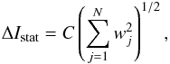$\begin{array}{ccc}\mathrm{\Delta }{\mathit{I}}_{\mathrm{stat}}\mathrm{=}\mathit{C}{\left(\sum _{\mathit{j}\mathrm{=}\mathrm{1}}^{\mathit{N}}{\mathit{w}}_{\mathit{j}}^{\mathrm{2}}\right)}^{\mathrm{1}\mathit{/}\mathrm{2}}\mathit{,}& & \end{array}$where C is the normalizing coefficient, w_j is the weight of the j-th particle, and N is the number of Monte Carlo particles in the bin (in the case of equal particle weights w, we obtain $\mathrm{\Delta }{\mathit{I}}_{\mathrm{stat}}\mathrm{=}\mathit{Cw}\sqrt{\mathit{N}}$ as per Poisson statistics).

The error due to binning stems from the fact that we fit histograms that we obtain by distributing Monte Carlo particles by their energy into different energy bins. This error for a given energy bin can be calculated from the following: 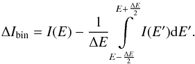$\begin{array}{ccc}\mathrm{\Delta }{\mathit{I}}_{\mathrm{bin}}\mathrm{=}\mathit{I}\mathrm{\left(}\mathit{E}\mathrm{\right)}\mathrm{-}\frac{\mathrm{1}}{\mathrm{\Delta }\mathit{E}}\underset{\mathit{E}\mathrm{-}\frac{\mathrm{\Delta }\mathit{E}}{\mathrm{2}}}{\overset{\mathit{E}\mathrm{+}\frac{\mathrm{\Delta }\mathit{E}}{\mathrm{2}}}{\mathrm{\int }}}\mathit{I}\mathrm{\left(}{\mathit{E}}^{\mathrm{\prime }}\mathrm{\right)}\mathrm{d}{\mathit{E}}^{\mathrm{\prime }}\mathit{.}& & \end{array}$Expanding the integrand into the Taylor series up to second order and assuming that I(E) ∝ E^{− β}, one can obtain 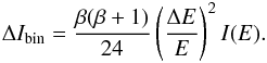$\begin{array}{ccc}\mathrm{\Delta }{\mathit{I}}_{\mathrm{bin}}\mathrm{=}\frac{\mathit{\beta }\mathrm{(}\mathit{\beta }\mathrm{+}\mathrm{1}\mathrm{)}}{\mathrm{24}}{\left(\frac{\mathrm{\Delta }\mathit{E}}{\mathit{E}}\right)}^{\mathrm{2}}\mathit{I}\mathrm{\left(}\mathit{E}\mathrm{\right)}\mathit{.}& & \end{array}$Both errors can be combined to give $\begin{array}{ccc}\mathrm{\Delta }\mathit{I}\mathrm{=}{\mathrm{(}\mathrm{\Delta }{\mathit{I}}_{\mathrm{stat}}^{\mathrm{2}}\mathrm{+}\mathrm{\Delta }{{\mathit{I}}_{\mathrm{bin}}^{\mathrm{2}}}^{\mathrm{)}}}^{\mathrm{1}\mathit{/}\mathrm{2}}\mathit{,}& & \end{array}$

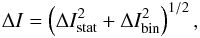
which was used in fitting the particle spectral data. For the CSA data, we estimated the statistical error is about an order of magnitude smaller than the error by binning, whereas for the SOLPACS data the statistical error prevails.

For a given parameter p of the fitting function, the fitting procedure (at energies E>E₀) gives the best-fit value, p_0,best and the standard deviation error, σ_p,fit. To take into account the systematic error due to the non-power-law form of the spectrum at low energies, we perform two additional fitting sessions by starting to fit from the energy E₀−ΔE and from E₀ + ΔE correspondingly, and calculate Δp = | p_best−p_0,best | for both additional fits. We take the largest $\mathrm{\Delta }{\mathit{p}}_{}$ and estimate the total error as $\begin{array}{ccc}{\mathit{\sigma }}_{\mathit{p}}\mathrm{=}{\mathrm{(}{\mathit{\sigma }}_{\mathit{p,}\mathrm{fit}}^{\mathrm{2}}\mathrm{+}\mathrm{\Delta }{\mathit{p}}^{\mathrm{2}}\mathrm{)}}^{\mathrm{1}\mathit{/}\mathrm{2}}\mathit{,}& & \end{array}$which is the value given in Table 1.

All Tables

All Figures

Fig. 1 Simulated particle energy spectra obtained with CSA (left panel) and SOLPACS (right panel) at t = 580 s for different values of the injection efficiency: ϵinj = 1.62 × 10-6 (blue circles), ϵinj = 5.40 × 10-6 (red circles), and ϵinj = 1.62 × 10-5 (green circles). Black curves represent fits to the spectral data, obtained with Eq. (15). The fitting was carried out at energies E> 0.2 MeV in all cases.

In the text

	Fig. 2 Distribution of particles in the foreshock at different energies, resulting from CSA (left panel, continuous curves) and SOLPACS (right panel, continuous curves) at the end (t = 580 s) of the simulation for ϵinj = 1.62 × 10-5 compared to Bell’s steady-state theory (dashed curves).
In the text

	Fig. 3 Time evolution of the spatial distribution of particles in the foreshock at E = 0.1 MeV (left panel) and E = 1.0 MeV (right panel) in SOLPACS. Dashed red and green curves in the right panel correspond to additional times t = 195 s and 235s.
In the text

Fig. 4 Wave intensity spectra obtained with CSA (left column) and SOLPACS (right column) for ϵinj = 1.62 × 10-5 at distance x = 0.0035 R⊙ (top row) and x = 0.13 R⊙ (bottom row) in front of the shock at t = 580 s. The filled blue and red circles in the SOLPACS data plots denote wave intensities of Alfvén waves of the opposite circular polarization. In all plots, coloured dashed lines show spectral indices and black dashed line shows the initial spectrum, normalized to provide λ = 1 R⊙ for 100 keV protons.

In the text

	Fig. 5 Proton mean free path as a function of distance from the shock, calculated for different energies for ϵinj = 1.62 × 10-5 at t = 580 s. Left panel: CSA (continuous curves) vs. steady-state theory (dashed curves); right panel: SOLPACS (continious curves) vs. steady-state theory (dashed curves).
In the text

	Fig. 6 Time evolution of the proton mean free path in the foreshock at E = 0.1 MeV in CSA (left panel) and SOLPACS (right panel) for ϵinj = 1.62 × 10-5.
In the text

	Fig. 7 Proton mean free path as a function of energy in the vicinity of the shock obtained with SOLPACS for different values of the injection parameter: ϵinj = 1.62 × 10-6 (blue), ϵinj = 5.40 × 10-6 (red) and ϵinj = 1.62 × 10-5 (green) at t = 580 s. Dashed line corresponds to the mean free path in the background plasma with the wave spectrum Iw ∝ k− 3/2 (λ ∝ E1/4).
In the text

	Fig. 8 Left panel: cut-off energy Ec versus injection efficiency ϵinj, resulting from the simulations and steady-state theory. Dashed curve represents a power-law extrapolation of SOLPACS results to larger values of ϵinj. Right panel: cut-off steepness δ versus injection efficiency ϵinj, resulting from the simulations.
In the text

References

- Afanasiev, A., & Vainio, R. 2013, ApJS, 207, 29 [Google Scholar]
- Afanasiev, A., Vainio, R., & Kocharov, L. 2014, ApJ, 790, 36 [Google Scholar]
- Axford, W. I., Leer, E., & Skadron, G. 1977, Proc. 15th Int. Cosmic Roy. Conf., 11, 132 [Google Scholar]
- Battarbee, M. 2013, Ph.D. Thesis, University of Turku, Finland [Google Scholar]
- Battarbee, M., Laitinen, T., & Vainio, R. 2011, A&A, 535, A34 [NASA ADS] [CrossRef] [EDP Sciences] [Google Scholar]
- Battarbee, M., Vainio, R., Laitinen, T., & Hietala, H. 2013, A&A, 558, A110 [NASA ADS] [CrossRef] [EDP Sciences] [Google Scholar]
- Bell, A. R. 1978, MNRAS, 182, 147 [NASA ADS] [CrossRef] [Google Scholar]
- Blandford, R. D., & Ostriker, J. P. 1978, ApJ, 221, L29 [Google Scholar]
- Ellison, D. C., Baring, M. G., & Jones, F. C. 1995, ApJ, 453, 873 [Google Scholar]
- Giacalone, J., & Jokipii, J. R. 2006, J. Phys. Conf. Ser., 47, 160 [NASA ADS] [CrossRef] [Google Scholar]
- Gordon, B. E., Lee, M. A., Möbius, E., & Trattner, K. J. 1999, J. Geophys. Res., 104, 28263 [NASA ADS] [CrossRef] [Google Scholar]
- Jokipii, J. R. 1966, ApJ, 146, 480 [Google Scholar]
- Jones, F. C., & Ellison, D. C. 1991, Space Sci. Rev., 58, 259 [NASA ADS] [CrossRef] [Google Scholar]
- Krymskii, G. F. 1977, Akademiia Nauk SSSR Doklady, 234, 1306 [NASA ADS] [Google Scholar]
- Lee, M. A. 1983, J. Geophys. Res., 88, 6109 [NASA ADS] [CrossRef] [Google Scholar]
- Lee, M. A. 2005, ApJS, 158, 38 [NASA ADS] [CrossRef] [Google Scholar]
- Lee, M. A., & Ip, W.-H. 1987, J. Geophys. Res., 92, 11041 [NASA ADS] [CrossRef] [Google Scholar]
- Li, G., Zank, G. P., & Rice, W. K. M. 2003, J. Geophys. Res., 108, 1082 [CrossRef] [Google Scholar]
- Li, G., Zank, G. P., & Rice, W. K. M. 2005, J. Geophys. Res., 110, 6104 [CrossRef] [Google Scholar]
- Ng, C. K., & Reames, D. V. 1995, ApJ, 453, 890 [NASA ADS] [CrossRef] [Google Scholar]
- Ng, C. K., & Reames, D. V. 2008, ApJ, 686, L123 [NASA ADS] [CrossRef] [Google Scholar]
- Schlickeiser, R., Vainio, R., Böttcher, M., et al. 2002, A&A, 393, 69 [NASA ADS] [CrossRef] [EDP Sciences] [Google Scholar]
- Tylka, A. J., & Dietrich, W. F. 2009, 31st ICRC Proc. [Google Scholar]
- Vainio, R., & Laitinen, T. 2007, ApJ, 658, 622 [NASA ADS] [CrossRef] [Google Scholar]
- Vainio, R., & Laitinen, T. 2008, J. Atmospheric and Solar-Terrestrial Physics, 70, 467 [Google Scholar]
- Vainio, R., & Schlickeiser, R. 1998, A&A, 331, 793 [NASA ADS] [Google Scholar]
- Vainio, R., Pönni, A., Battarbee, M., et al. 2014, J. Space Weather and Space Climate, 4, A8 [Google Scholar]
- Zank, G. P., Rice, W. K. M., & Wu, C. C. 2000, J. Geophys. Res., 105, 25079 [NASA ADS] [CrossRef] [Google Scholar]