| Issue |
A&A
Volume 584, December 2015
|
|
|---|---|---|
| Article Number | A9 | |
| Number of page(s) | 18 | |
| Section | Planets and planetary systems | |
| DOI | https://doi.org/10.1051/0004-6361/201525690 | |
| Published online | 13 November 2015 | |
Microwave thermal emission from the zodiacal dust cloud predicted with contemporary meteoroid models
Faculty of Physics, Bielefeld University, Postfach 100131, 33501 Bielefeld, Germany
e-mail: vdikarev@physik.uni-bielefeld.de
Received: 19 January 2015
Accepted: 2 July 2015
Predictions of the microwave thermal emission from the zodiacal dust cloud are made using several contemporary meteoroid models to construct the distributions of the cross-section area of dust in space, and by applying the Mie light-scattering theory to estimate the temperatures and emissivities of dust particles in a wide range of sizes and heliocentric distances. In particular, the Kelsall model of the zodiacal light emission based on COBE infrared observations is extrapolated to the microwaves with assistance from fits to selected IRAS and Planck data. Furthermore, the five populations of interplanetary meteoroids by Divine and the Interplanetary Meteoroid Engineering Model (IMEM) based on a variety of remote and in situ observations of dust are used in combination with the optical properties of olivine, carbonaceous, and iron spherical particles. The Kelsall model has been accepted by the cosmic microwave background (CMB) community for subtraction of the zodiacal cloud’s foreground emission. We show, however, that the Kelsall model predicts microwave emission from interplanetary dust that is remarkably different from the results obtained by applying the meteoroid engineering models. We make maps and spectra of the microwave emission predicted by all three models assuming different compositions of dust particles. The predictions can be used to look for the emission from interplanetary dust in CMB experiments and to plan new observations.
Key words: radiation mechanisms: thermal / zodiacal dust / cosmic background radiation
© ESO, 2015
1. Introduction
The unprecedentedly high-precision surveys of the microwave sky performed recently by the Wilkinson Microwave Anisotropy Probe (WMAP, Bennett et al. 2013) and Planck (Planck Collaboration I 2014) observatories in search of – and for the characterization of – the large- and small-scale structures of the cosmic microwave background (CMB) anisotropies pose new challenges for the simulation and subtraction of the foreground emission sources, including the solar system dust. Previous templates designed for this purpose were based on the Kelsall et al. (1998) model. These templates indicated little significance of the interplanetary dust for the WMAP survey (Schlegel et al. 1998), yet a remarkable contribution was detected at high frequencies of Planck (Planck Collaboration XIV 2014).
The angular power spectrum of CMB anisotropies is in good agreement with the inflationary Λ-cold dark matter model (Planck Collaboration I 2014). However, the reconstructed CMB maps at the largest angular scales reveal some intriguing anomalies, among them unexpected alignments of multipole moments, in particular with directions singled out by the solar system (Schwarz et al. 2004). The quadrupole and octopole are found to be mutually aligned and they define axes that are unusually perpendicular to the ecliptic pole and parallel to the direction of our motion with respect to the rest frame of the CMB (the dipole direction). For reviews see Bennett et al. (2011), Copi et al. (2010), Bennett et al. (2013), and Planck Collaboration XXIII (2014), as well as Copi et al. (2015b) for a detailed analysis of the final WMAP and first Planck data. It has been suggested that an unaccounted observational bias may persist, for example, yet another foreground source of the microwave emission bound to the solar system. Dikarev et al. (2009) explored the possibility that the solar system dust emits more than was previously thought, and found that the macroscopic (> 0.1 mm in size) meteoroids can contribute ~ 10 μK in the microwaves, i.e., comparable with the power of the CMB anomalies, without being detected in the infrared (IR) light and without being included in the IR-based models like that of Kelsall et al. (1998). Babich et al. (2007) and Hansen et al. (2012) have also studied the possible contribution of the Kuiper belt objects to the microwave foreground radiation. Dikarev et al. (2008) constructed some dust emission templates and tested them against the WMAP data.
Here we improve and extend the preliminary estimates of Dikarev et al. (2009). In addition to the Kelsall model, we use two meteoroid engineering models to make accurate and thorough maps of the thermal emission from the zodiacal cloud in the wavelength range from 30 μm to 30 mm.
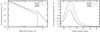 |
Fig. 1 Profiles of particle cross-section area density predicted with selected meteoroid models and compared with each other: ecliptic radial (left) and latitudinal at 1 AU from the Sun (right, the vernal equinox is at latitude 0°). |
The paper is organized as follows. Section 2 introduces three models of the interplanetary meteoroid environment that we use to predict the thermal emission from the zodiacal dust cloud. A detailed description of the theory and observations incorporated in each model is provided, which may be helpful not only for cosmologists interested in understanding the solar system microwave foregrounds, but also for developers of new meteoroid models who would like to comprehend earlier designs. Section 3 describes the thermal emission models. Empirical models as well as the Mie light-scattering theory are used to calculate the temperatures and emission intensities of spherical dust particles composed of silicate, carbonaceous, and iron materials, for broad ranges of size and heliocentric distance. The models of the spatial distribution of dust and thermal emission are combined in Sect. 4 in order to make all-sky maps and spectra of the thermal emission from the interplanetary dust. Conclusions are drawn in Sect. 5.
Throughout this paper, we deal mostly with the wavelengths, since the dust optical properties are naturally described in terms of linear scales. The CMB community, however, is more accustomed to frequencies. A conversion table is therefore useful for the observation wavebands of infrared detectors and radiometers. It can be found in the Appendix.
2. Meteoroid models
In this paper, we use three recent and contemporary models of the zodiacal dust cloud developed by Kelsall et al. (1998), Divine (1993), and Dikarev et al. (2005a). The first model is constrained by the infrared observations from the Earth-orbiting satellite COBE (hereafter the Kelsall model). The Kelsall model is most familiar to and most often used by the cosmic microwave background (CMB) research community as it was designed to assess and mitigate the contamination of the background radiation maps by the foreground radiation from interplanetary dust. The other two models incorporate data obtained by diverse measurement techniques and serve to predict meteoroid fluxes on spacecrafts and to assess impact hazards. Because they are mostly applied in spacecraft design and analysis, they are often called the meteoroid engineering models. We chose the Divine model and the Interplanetary Meteoroid Engineering Model (IMEM). We also check whether the most recent NASA meteoroid engineering model, MEM (McNamara et al. 2004), can be used in our study, and explain why it cannot be.
The Kelsall model does not consider the size distribution of particles in the zodiacal cloud. The size distribution is implicitly presented by the integral optical properties of the cloud. In contrast, the meteoroid engineering models are obliged to specify the fluxes of meteoroids for various mass, impulse, or other level-of-damage thresholds, hence they explicitly provide the size distribution.
Profiles of particle cross-section area density per unit volume of space are plotted for the Kelsall and Divine models and for IMEM in Fig. 1. Interestingly, the Kelsall model is sparser than the other two models at most heliocentric distances. The meteoroid engineering models predict substantially more dust than Kelsall does, especially beyond 1 AU from the Sun: Divine’s density is almost flat in the ecliptic plane between 1 and 2 AU, exceeding Kelsall’s density by a factor of 3 in the asteroid belt. The IMEM density remains similar to that of the Kelsall model up to ~ 3 AU, showing a local maximum beyond the asteroid belt near 5 AU from the Sun, in the vicinity of Jupiter’s orbit. IMEM possesses a somewhat narrower latitudinal distribution than that of the Kelsall and Divine models.
All these distinctions stem from different observations and physics incorporated in the different models. When describing them in subsequent subsections, we do not aim to select the best model. Instead, we take all three of them with the intention of “bracketing” the most complex reality by three different perspectives from the different “points of view”.
2.1. The Kelsall model
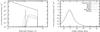 |
Fig. 2 Radial and latitudinal profiles of particle cross-section area density in the Kelsall model, component by component. |
A concise analytical description of the infrared emission from the interplanetary dust captured by the COBE Diffuse InfraRed Background Experiment (DIRBE) was proposed by Kelsall et al. (1998). Five emission components are recognized: a broad, bright smooth cloud; three finer and dimmer dust bands; and a circumsolar dust ring along the Earth orbit with an embedded Earth-trailing blob. Each component is described by a parameterized empirical three-dimensional density function specifying the total cross-section area of the component’s dust particles per unit volume of space (Fig. 2), and by their collective light scattering and emission properties such as albedo and absorption efficiencies. The particle size distributions of the components are not considered. Most of the light scattering and emission properties are neither adopted from laboratory studies of natural materials nor predicted by theories of light scattering; instead, they are free parameters of the model fit to the DIRBE observations.
The smooth cloud is the primary component of the Kelsall model. Its density function is traditionally separated into radial and vertical terms. The radial term is a power law  with α = 1.34 ± 0.022 being the slope of the density decay with distance from the cloud’s center Rc. The slope is known to be equal to one for the dust particles in circular orbits migrating toward the Sun under the Poynting-Robertson drag. While orbiting the Sun, the particles absorb its light coming from a slightly forward direction due to aberration, and the radiation pressure force has a non-zero projection against the direction of their motion; this projection causes gradual loss of the orbital energy and decrease of the semimajor axis of particle’s orbit. The slope is greater than one if the particle orbits are initially eccentric, or if the zodiacal cloud is fed from sources broadly distributed over radial distances, so that the inner circles of the cloud are supplied from more dust sources than the outer circles (Leinert et al. 1983; Gor’kavyi et al. 1997).
The vertical term of smooth cloud’s density is represented by a widened, modified fan model. The smooth cloud’s symmetry plane is inclined off the ecliptic plane. This happens because the Earth has no influence on the orbital dynamics of the vast majority of cloud particles. The giant planets, Jupiter primarily, perturb the orbits of dust particles as well as their sources or parent bodies, such as comets and asteroids, and control the inclinations of the orbits of the particles. An offset of the center of the cloud from the Sun is also allowed in the Kelsall model (on the order of 0.01 AU). The vertical motion of the Earth with respect to the cloud’s symmetry plane leads to the modulations of the infrared emission from the zodiacal cloud reaching 30% in the ecliptic polar regions.
The dust bands are the remnants of collisional disruptions of asteroids that resulted in formation of the families of asteroids in similar orbits and remarkable dust belts. The dust bands were discovered first on the high-resolution maps made by the IRAS satellite (Low et al. 1984) and recognized later in the COBE DIRBE data as well. Kelsall et al. (1998) introduced three dust bands in their model, attributed to the Themis and Koronis asteroid families ( ecliptic latitude), the Eos family (± 10°), and the Maria/Io family (± 15°). The bands have symmetry planes different from that of the smooth background cloud. The bands are all double, with the density peaking above and below the respective symmetry plane since their constituent particles retain the inclination of the ancestor asteroid orbit, but the longitudes of nodes get randomized by the planetary perturbations. The vertical motion of such particles is similar to that of an oscillator, which moves slower and spends more time near its extremities, thus the density at the latitudes of each family’s orbital inclination is high. One would expect a similarly shaped “edge-brightened” radial density with the peaks at the perihelion and aphelion distances of the parent body orbit (e.g., Sect. 3 in Gor’kavyi et al. 1997). However, the dust in asteroid bands is proven to be migrating toward the Sun under the Poynting-Robertson drag; Reach (1992) has demonstrated that the temperatures of particles and parallaxes of the bands measured from the moving Earth are both higher than those expected in the respective asteroid families of their origin, implying that the bands extend farther toward the Sun than their ancestor bodies. Unlike Reach (1992), Kelsall et al. (1998) only allowed for a partial migration of dust by introducing a cut-off at a minimal heliocentric distance either defined or inferred individually for each band. They also fixed rather than inferred most of the dust band shape parameters. It is noteworthy that Kelsall et al. (1998) did not introduce an explicit outer cut-off for the densities of the smooth cloud and dust bands. Instead, they integrated the densities along the lines of sight from the Earth to the maximum heliocentric distance of 5.2 AU (close to the Jovian orbital radius).
The dust particles on nearly circular orbits migrating under the Poyinting-Robertson drag toward the Sun are temporarily trapped in a mean-motion resonance with the Earth near 1 AU (Dermott et al. 1984). The resulting enhancement of the zodiacal cloud density is described in the Kelsall model by the solar ring and Earth-trailing blob. The trailing blob is the only component of the model that is not static: it is orbiting the Sun along a circular orbit with a period of one year, and as the name suggests, its density peak is located behind the moving Earth. The solar ring and trailing blob have density peak distances slightly outside the Earth orbit, their symmetry planes are inclined off the ecliptic plane, and the trailing blob orbits the Sun at a constant velocity whereas the Earth velocity is variable due to the eccentricity of our planet’s orbit. Consequently, the Earth moves with respect to the solar ring and trailing blob over the course of the year much like the other components of the Kelsall model.
The DIRBE instrument performed a simultaneous survey of the sky in ten wavelength bands at 1.25, 2.2, 3.5, 4.9, 12, 25, 60, 100, 140, and 240 μm. It was permitted to take measurements anywhere between the solar elongations of 64° and 124°. As the Earth-bound COBE observatory progressed around the Sun, DIRBE took samples of the infrared background radiation from all over the sky. The foreground radiation due to interplanetary dust was a variable ingredient of the sky brightness because it depends on the changing position of observatory with respect to the cloud. Thus, the fitting technique was based on minimizing the difference between the brightness variations in time observed along independent lines of sight and those predicted by the Kelsall model for the same lines of sight, ignoring the underlying photometric baselines contaminated or even dominated by the background sources.
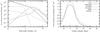 |
Fig. 3 Radial and latitudinal profiles of particle cross-section area density in the Divine model, component by component. |
The accuracy of the Kelsall model in describing the infrared emission from interplanetary meteoroids in DIRBE’s wavelength bands and within the range of permitted solar elongations is reported to be better than 2%. Interpolations of the model brightnesses between the instrument wavelengths and extrapolations beyond the wavelength and solar elongation ranges may be prone to higher uncertainties. Indeed, the concise description of the zodiacal emission contribution to the DIRBE data provides no clue as to how the light scattering and emission properties of its components depend on wavelength between and beyond the ten DIRBE wavelength bands.
When applying the Kelsall model in the far-infrared wavelengths and microwaves, one should bear in mind that Kelsall et al. (1998) already found the 140 and 240 μm bands nearly useless in constraining the density distribution parameters owing to relatively high detector noise and the small contribution of the radiation from the interplanetary dust at these wavelengths. Consequently, the inferred parameters of the density distributions in the Kelsall model are based on the observations at the wavelengths up to 100 μm. The dust particles are efficient in interacting with the electromagnetic radiation if their sizes are not too small with respect to the wavelength (2πs>λ, where s is the particle radius and λ is the wavelength). Dust grains with radii from ~16 μm are therefore visible at the wavelength of 100 μm. Dikarev et al. (2009) argue that a considerable number of meteoroids are present in the solar system with sizes bigger than ~100 μm that are outshined in the infrared light by more abundant and ubiquitous smaller dust grains. The longest observation wavelength of DIRBE at which Kelsall et al. (1998) could still constrain the density distributions of dust is short of being capable to resolve these particles unless they compose distinctive features like dust bands.
We use the formulae for the density functions provided by Planck Collaboration XIV (2014) since the original paper by Kelsall et al. (1998) contains typographical misprints in the definitions of the asteroid dust band and circumsolar ring densities.
2.2. The Divine model
A model of the interplanetary meteoroid environment (Divine 1993) constructed to predict fluxes on spacecraft anywhere in the solar system from 0.05 to 40 AU from the Sun, is composed of five distinct populations, each of which has mathematically separable distributions in particle mass and in orbital inclination, perihelion distance, and eccentricity (Fig. 3). Using the distributions in orbital elements, Divine explicitly incorporated Keplerian dynamics of meteoroids in heliocentric orbits.
The Divine model is constrained by a large number of diverse meteoroid data sets. The mass distribution of meteoroids from 10-18 to 102 g is fitted to the interplanetary meteoroid flux model (Grün et al. 1985), which in turn is based on the micro-crater counts on lunar rock samples retrieved by the Apollo missions, i.e., the natural surfaces exposed to the meteoroid flux near Earth, and data from several spacecraft. The orbital distributions are determined using meteor radar data, observations of zodiacal light from the Earth as well as from the Helios and Pioneer 10 interplanetary probes, and meteoroid fluxes measured in situ by impact detectors on board Pioneer 10 and 11, Helios 1, Galileo and Ulysses spacecraft at the heliocentric distances ranging from 0.3 to 18 AU. The logarithms of the model-to-data ratios were minimized in a root-mean-square sense. When modeling the zodiacal light, Divine assumed that the scattering function is independent of meteoroid mass. The albedos of dust particles were defined somewhat arbitrarily in order to hide the populations necessary to fit the in situ measurements from the zodiacal light observations. No infrared observations were used to constrain the model.
The core population is the backbone of the Divine model, it fits as much data as possible with a single set of distributions. The distribution in perihelion distance rπ of the core-population particles can be used as strictly proportional to  up to 2 AU from the Sun. This function resembles a spatial concentration, and its slope is close to Kelsall’s α = 1.34 for the radial density term: much like the infrared data from COBE, the zodiacal light observations from the Earth and interplanetary probes demand that the slope be steeper than a unit exponent. The eccentricities are moderate (peaking at 0.1 and mostly below 0.4), inclinations are small (mostly below 20°).
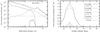 |
Fig. 4 Radial and latitudinal profiles of particle cross-section area density in IMEM, component by component. The density plots are not smooth since the orbital distributions in IMEM are approximated by step functions. |
The other populations fill in the gaps where one population with separable distributions is not sufficient to reproduce the observations. Their names hint at distinctive features of their orbital distributions. The inclined population is characterized by inclinations largely in the range 20°–60°, its eccentricities are all below 0.15. In contrast, the eccentric population is composed of particles in highly eccentric orbits (the eccentricities are largely between 0.8 and 0.9), the inclinations are same as in the core population. These two populations are added in order to compensate for a deficit of meteoroids from the core population with respect to in situ flux measurements on board the Helios spacecraft. (The eccentric population is also used to match the interplanetary flux model between 10-18 and 10-15 g.) The halo population has a uniform distribution of orbital plane orientations and “surrounds” the Sun as a halo between roughly 2 and 20 AU. It patches the meteoroid model where the above-listed populations are not sufficient to reproduce the Ulysses and Pioneer in situ flux measurements. The eccentric, inclined and halo populations are composed of meteoroids much smaller than those significant enough for predictions of the infrared and microwave observations.
The asteroidal population is described last but it makes a huge difference between Kelsall’s and Divine’s models. Already when fitting the first population to the meteor radar data, Divine observed that the results for the distribution in perihelion distance show a minimum near rπ = 0.6 AU, suggesting that two components are involved (i.e., inner and outer). The radial slope of the inner component was consistent with that demanded by the zodiacal light observations, and the inner and outer components contributed 45% and 55%, respectively, to the flux near Earth. The outer component’s concentration peaked outside the Earth orbit, in the asteroid belt. Since the main contribution to the zodiacal light comes from the particles with masses smaller than 10-5 g and the median meteoroid mass of the meteor radar was 10-4 g, it was reasonable to ascribe the inner fraction to a population dominated by smaller particles responsible for the zodiacal light, and the outer fraction to another one dominated by larger particles detected as meteors only with the radar. The two fractions were divided into the core and asteroidal populations, accordingly. Their inclination and eccentricity distributions are identical, but the distributions in perihelion distance and mass are different. The asteroidal population is used to fit the interplanetary flux model at masses > 10-4 g.
Derived from data analysis rather than postulated theoretically, the distinction between the core and asteroidal populations in the Divine model separates – both on the mass and perihelion distance scales – the small dust particles migrating toward the Sun under the Poynting-Robertson drag, the concentration of which increases with the decrease of the heliocentric distance, and their immediate parent bodies, the larger particles swarming further away from the Sun, i.e., in the asteroid belt according to Divine (1993).
2.3. IMEM
The Interplanetary Meteoroid Engineering Model (IMEM) was developed for ESA by Dikarev et al. (2005a). Like the Divine model, it uses the distributions of orbital elements and mass rather than the spatial density functions of the Kelsall model, ensuring that the dust densities and fluxes are predicted in accord with Keplerian dynamics of the constituent particles in heliocentric orbits. Expansion of computer memory has also enabled the authors of IMEM to work with large arrays representing multi-dimensional distributions in orbital elements to replace Divine’s separable distributions. The distribution in mass remains separable from the three-dimensional distribution in inclination, perihelion distance, and eccentricity.
IMEM is a major revision of the Divine-Staubach meteoroid model, which was also developed for ESA and described in Staubach et al. (1997) and Grün et al. (1997). IMEM has inherited a population of interstellar dust from that model. It is represented by a monodirectional stream of tiny dust particles (less than ~ 10-9 g in mass) flowing through the solar system and having constant number density and velocity.
IMEM is constrained by the micro-crater size statistics collected from the lunar rocks retrieved by the Apollo crews; COBE DIRBE observations of the infrared emission from the interplanetary dust at 4.9, 12, 25, 60, and 100 μm wavelengths; and Galileo and Ulysses in situ flux measurements. An attempt to incorporate new meteor radar data from the Advanced Meteor Orbit Radar (AMOR, see Galligan & Baggaley 2004) was not successful (Dikarev et al. 2004); the latitudinal number density profile of meteoroids derived from the meteor radar data stood in stark contrast to that admissible by the COBE DIRBE data, which was due to an incomplete understanding of the observation biases.
The interplanetary meteoroids in IMEM are distributed in orbital elements following an approximate physical model of the origin and orbital evolution of particulate matter under planetary gravity, the Poynting-Robertson effect, and mutual collisions. Grün & Dikarev (2009) visualize the IMEM distributions of meteoroids in mass and in orbital elements in graph and color plots. The cross-section area density profiles are shown in Fig. 4.
All interplanetary meteoroids are divided into populations by origin/source and mass/dynamical regime. Grün et al. (1985) constructed a model of the mass distribution of interplanetary meteoroids. Based on this model, they estimated particle lifetimes against two destructive processes, mutual collisions and migration downward toward the Sun due to the Poynting-Robertson drag (terminated by particle evaporation or thermal break-up). Figure 5 shows that the lifetime against mutual collisions is shorter than the Poynting-Robertson time for the meteoroids bigger than ~ 10-5 g in mass, located at 1 AU from the Sun. The rate of destruction of meteoroids (by the same process) increases or decreases by a factor of ten just one order of magnitude away from this transition mass in either direction. The rates vary with the distance from the Sun; however, the transition mass remains nearly unchanged (Fig. 6 in Grün et al. 1985), which is why Dikarev et al. (2005a) were able to simplify the problem by dividing the mass range into two subranges with distinct mass distribution slopes and dynamics. Meteoroids below the transition mass of 10-5 g are treated as migrating from the sources toward the Sun under the Poynting-Robertson drag; meteoroids above the transition mass are assumed to retain the orbits of their ultimate ancestor bodies over their short lifetimes until collisional destruction.
The ultimate ancestor bodies of interplanetary dust in IMEM are comets and asteroids. A catalogue of asteroids is used to account for the latter source of meteoroids. Three distinct populations of asteroids are recognized and allowed to have independent total production rates: the Themis and Koronis families (semimajor axes 2.8 <a< 3.25 AU, eccentricities 0 <e< 0.2, and inclinations  ), Eos and Veritas families (2.95 <a< 3.05 AU, 0.05 <e< 0.15,
  ), and the main belt (a< 2.8 AU). The orbital distributions of meteoroids more than 10-5 g in mass are constructed by counting the numbers of catalogued asteroids per orbital space bins. The orbital distributions of meteoroids less than 10-5 g in mass are described as the flow of particles along the Poynting-Robertson evolutionary paths (Gor’kavyi et al. 1997) starting from the source distributions defined earlier. The mass distributions are adopted from the interplanetary meteoroid flux model by Grün et al. (1985) for each mass range as shown in Fig. 5.
The orbital distributions of meteoroids from comets cannot be defined as easily as those of meteoroids from asteroids. Because of a number of loss mechanisms, such as comet nuclei decay, accretion, tidal disruption, or ejection from the solar system by planets, very few comets are active at a given epoch and listed in the catalogues. Moreover, the catalogues are prone to observation biases since the comet nuclei are revealed by gas and dust shed at higher rates at lower perihelion distances.
In order to describe the orbital distributions of meteoroids of cometary origin, Dikarev & Grün (2004) proposed an approximate analytical solution of the problem of a steady-state distribution of particles in orbits with frequent close encounters with a planet. This solution is applied in order to represent the orbital distributions of meteoroids from comets in Jupiter-crossing orbits, i.e., the vast majority of catalogued comets. Big meteoroids with masses greater than 10-5 g are confined to the region of close encounters with Jupiter. There is only one quantity that is approximately conserved in the region of close encounters with Jupiter. It is the Tisserand parameter T with aJ being the semimajor axis of Jovian orbit. The numbers of meteoroids in T-layers are therefore stable over a long period of time. They are free parameters to be determined from the fit of IMEM to observations. The relative distributions in orbital elements within each T-layer are found theoretically (Dikarev & Grün 2004).
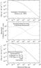 |
Fig. 5 Cumulative mass distribution of interplanetary meteoroids (Grün et al. 1985, top); meteoroid lifetimes against mutual collisions and Poynting-Robertson drag (middle); and cumulative mass distributions of meteoroid populations in IMEM (Dikarev et al. 2005a, bottom) including the interstellar dust, which is ignored in this paper owing to the tiny sizes of the constituent particles. The flux of meteoroids with m> 10-5 g is lower in IMEM than in the Grün model since the impact velocities of big meteoroids are higher at 1 AU from the Sun in IMEM and they produce larger craters on the lunar rocks than in the Grün model, which assumed a single impact velocity for all meteoroid sizes. |
Finer dust grains with masses less than 10-5 g leak from this region into the inner solar system and then migrate toward the Sun under the Poynting-Robertson drag. The Poynting-Robertson migration time is much longer than the close approach time in the region of close encounters with Jupiter, consequently, the orbital distributions of all meteoroids are shaped there by the gravitational scattering on Jupiter. It is only the dust leaking through the inner boundary of the region that is distributed as the flow of particles along the Poynting-Robertson evolutionary paths (Gor’kavyi et al. 1997). Their distributions are also established theoretically in IMEM, with the normalization factors being inferred from the fit to observations.
An empirical finding by Divine of a helpful separation of the bulk of the meteoroid cloud into the core and asteroidal populations – i.e., the segregation of big and small dust particles – has become one of the physical assumptions in IMEM.
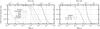 |
Fig. 6 Cumulative distribution functions of particle cross-section area in mass (size) for each population of the interplanetary meteoroid model by Divine (1993) and IMEM (Dikarev et al. 2005a). The material density of particles is equal to 2.5 g cm-3 in both models except Divine’s eccentric population where it is ten times lower. The particle size scale should not be used in combination with the plot for the latter population. |
The weights of populations of dust from comets, asteroids, and interstellar space in IMEM were fitted to in situ flux measurements using the Poisson maximum-likelihood estimator and to infrared observations using the Gaussian maxiumum-likelihood estimator. The population of interstellar dust from the Divine-Staubach model was renormalized only. The relative mass distribution and velocity of interstellar particles were not changed.
IMEM was tested against those data not incorporated in the model by Dikarev et al. (2005b), confirming that the orbital evolution approach allows for more reliable extrapolations of the observations and measurements incorporated in the model; it is compared with several other meteoroid models by Drolshagen et al. (2008).
2.4. MEM
The Meteoroid Engineering Model (MEM) described by McNamara et al. (2004) is another recent development in orbital distributions and software used to predict fluxes on spacecraft in the solar system and near Earth. It is constrained by the Earth-based meteor radar data CMOR (Canadian Meteor Orbit Radar) and zodiacal light observations from two interplanetary probes, Helios 1 and 2. The nominal heliocentric distance range at which the model is applicable, from 0.2 to 2 AU, is rather limited, however. Even though the meteoroid mass range of 10-6 to 10 g covered by the model is extremely interesting for the purposes of our study, some assumptions made by the authors are rather arguable. In particular, the mutual collisions between meteoroids are considered in the model ignoring the dependence of the meteoroid collision probability on its size, whereas Grün et al. (1985) calculated that the lifetime against collisional disruption of meteoroids varies by a factor of 100 between the masses of 10-6 and 1 g (their Fig. 6 and our Fig. 5). It is not only the mass distribution of particles that is determined by the collision probability, but also the orbital distributions: as the lifetime against collisions becomes shorter than the Poynting-Robertson time by orders of magnitude, the meteoroids can no longer survive a journey from their sources toward the Sun and the orbital distributions of bigger particles are more similar to the distributions of their sources than are the distributions of smaller particles. MEM is unfortunately unable to reveal and describe this important feature of the interplanetary meteoroid cloud.
2.5. Cross-section area distributions
We used the notion of cross-section area density of meteoroids as self-explanatory. Indeed, Kelsall et al. (1998) made it the basic element of their model and named it simply “the three-dimensional density” nc(X,Y,Z) of model component c, with X, Y, and Z being the cartesian coordinates of position in the solar system. (It was measured in AU-1 though, unexpectedly enough for the term.)
The meteoroid engineering models do not define the cross-section area density directly; it must be derived from even more basic elements, and by doing so we can also clarify its meaning. The Divine model and IMEM provide us with the distributions of particles in mass and in orbital elements, from which the number density Nc(s,X,Y,Z) of the particles with sizes greater than s per unit volume of space can be determined (Divine 1993; Dikarev et al. 2005a). For a fixed position (X,Y,Z), Nc is proportional to the cumulative distribution function of meteoroids from population c in size s inside the model size range [smin,smax].
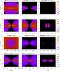 |
Fig. 7 Particle cross-section area densities (per unit volume of space, AU2/AU3) for each component or population of the meteoroid models by Kelsall et al. (1998), Divine (1993), and IMEM (Dikarev et al. 2005a). We note that two maps for the cometary dust in IMEM are plotted in a different scale. |
In order to obtain the cross-section area density of meteoroids nc one must convolve the partial derivative −∂Nc/∂s with the cross-section area of a single meteoroid of size s, which is equal to πs2, assuming that all particles are spherical, over the model size range  Now it is easy to see why nc is measured in AU-1: the number density per unit volume (AU-3) is multiplied by the cross-section measured in area units (AU2) under the integral sign, while the dimensions of ds in the numerator and ∂s in the denominator cancel out.
The integral of the cross-section area density along a line of sight (l.o.s.) gives its column density, i.e., the total cross-section area of particles inside an infinitesimally narrow column along the l.o.s. divided by the column cross-section area. This dimensionless ratio is equal to the optical depth of the cloud along that l.o.s., when the cloud is optically thin, and ignoring that the particle efficiencies in absorbing and scattering light can in fact be higher or lower than unity.
Cumulative distribution functions of meteoroid cross-section area in mass and size for each population of the meteoroid models by Divine (1993) and Dikarev et al. (2005a) are plotted in Fig. 6 (normalized to unity). We note that one population of the Divine model has an assumed material density of 0.25 g cm-3, whereas the standard value assumed for all other populations as well as in many other meteoroid models is 2.5 g cm-3.
Figure 7 maps the total cross-section area of dust particles per unit volume of space, as a function of the position in the solar system, for each component or population of every meteoroid model introduced in the previous section. The X and Z coordinates are measured from the Sun, with the X-axis pointing to the vernal equinox and Z-axis being perpendicular to the ecliptic plane.
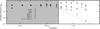 |
Fig. 8 Absorption efficiencies (“emissivity modification factors”, see text for explanation) of dust in the Kelsall model determined for the COBE DIRBE wavelengths by Kelsall et al. (1998), gray area on the plot, and for the Planck HFI wavelengths by Planck Collaboration XIV (2014). Fixsen & Dwek (2002) have also used the data from the COBE FIRAS instrument to determine the annually averaged spectrum of the zodiacal cloud plotted here with a dotted line. |
The Kelsall model is reproduced in the upper row of maps. Three dust bands are shown together in the middle plot. The smooth cloud is to the left, and the solar ring is to the right. The dominant component of the Kelsall model, the smooth cloud, increases in density only toward the Sun and the symmetry plane is slightly inclined off the ecliptic plane. The dust bands are the only component of the model bulking beyond the Earth orbit, and they are by definition bound to the ecliptic latitudes of their ancestor asteroid families’ orbit inclinations. Both the smooth cloud and the dust bands extend only up to the heliocentric distance of 5.2 AU, since Kelsall et al. (1998) stopped integrating the model densities there. A more rigorous model of the bands composed of dust migrating toward the Sun as a result of the Poynting-Robertson effect would put their densities’ cut-offs at the outer boundaries of the corresponding asteroid families. We note, however, that most of the thermal infrared emission from the interplanetary dust observed by COBE was due to the dust within 0.5−1 AU from the Earth orbit, since COBE could not be pointed too close to the Sun and dust is too cold and inefficient at thermal emission far from the Sun (Dikarev et al. 2009, their Sect. 2.1 and Fig. 2). Thus, for the purpose of modeling the infrared thermal emission observed from the Earth, the behavior of the density at multiples of an astronomical unit was not important, although this may not be the case for the microwave emission.
The next two rows of maps depict the populations of the Divine model. The core and asteroidal populations are important in the infrared and microwave emission ranges. Their distributions in space are remarkably different, with the core population density growing higher toward the Sun and the asteroidal population density peaking beyond the orbit of the Earth. The two populations are also composed of particles of different sizes: the core population is mostly smaller and the asteroidal population mostly bigger than ~ 50 μm. The halo, inclined and eccentric populations are provided for the sake of completeness. Their tiny particles (up to ~ 10 μm) are ignorable in the wavelength ranges of interest.
The bottom row of maps and the right map in the third row exhibit the populations from IMEM. The asteroidal dust particles bigger than 10-5 g in mass are confined to the asteroid belt. They are not migrating from their ancestor body orbits toward the Sun nor do they extend beyond the outer edge of the asteroid belt. The smaller dust particles move toward the Sun due to the Poynting-Robertson effect. The inclinations of their orbits are intact, since IMEM does not take into account any planetary perturbations other than gravitational scattering by Jupiter that require a close approach to the giant planet. Consequently, the latitudinal distribution of their density is independent on heliocentric distance away from the source region, i.e., asteroid belt.
Big cometary particles have a density peak along the orbit of Jupiter. This occurs because all their orbits are required by definition to approach the Jovian orbit within 0.5 AU or less. Small cometary particles leak through the inner boundary of the region of close encounters with Jupiter and migrate toward the Sun under the action of the Poynting-Robertson effect. They reach the highest density at the shortest heliocentric distances. A cometary dust density enhancement in the form of a spherical shell with a radius of 5.2 AU is a negligibly small defect caused by the assumption of a uniform distribution of particle orbits in longitudes of perihelia in IMEM. Concentric spherical “shells” of different densities on the map of cometary meteoroids with m> 10-5 g are due to finite discretization of the distribution in perihelion distance.
The Kelsall model bets on essentially single-population representation of the interplanetary meteoroid cloud, with the solar ring and dust bands being minor features (Fig. 2). The meteoroid engineering models, however, clearly show that the cloud is composed of different sorts of dust in major populations that are also distributed differently in space. We will see below how this affects the microwave emission predictions.
3. Thermal emission models
The thermal emission from dust particles is expressed with respect to the blackbody emission Bλ(T) at the wavelength λ and temperature T, using an emissivity modification factor that is equal to the absorption efficiency factor Qabs(s,λ) for the particle size s (Bohren & Huffman 1983). The factor of Qabs is defined as the ratio of the effective absorption cross-section area of the particle to its geometric cross-section area.
3.1. The Kelsall model
The light scattering and emission properties of dust are not defined in the Kelsall model for the wavelengths between and beyond those of the COBE DIRBE instrument. Figure 8 shows Kelsall’s emissivity modification factors, or absorption efficiencies in order to preserve the uniformity of terms, for the DIRBE wavelength bands. Planck Collaboration XIV (2014) used the cross-section area density of the Kelsall model and found that the absorption efficiencies for its components approximately describe the thermal emission from interplanetary dust at the wavelengths of Planck’s High Frequency Instrument (HFI). Fixsen & Dwek (2002) used the FIRAS (Far-Infrared Absolute Spectrometer) data from COBE and found that the annually averaged spectrum of the zodiacal cloud can be fitted with a single blackbody at a temperature of 240 K with an absorption efficiency that is flat at wavelengths shorter than 150 μm and Qabs ∝ λ-2 beyond 150 μm.
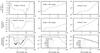 |
Fig. 9 Optical constants and absorption efficiencies for olivine and iron of Pollack et al. (1994), and for amorphous carbonaceous grains from the “BE” sample of Zubko et al. (1996) used in this paper, in addition to the data introduced by Dikarev et al. (2009). The absorption efficiencies are calculated for the sizes of spherical dust grains indicated in the bottom row of plots. |
The absorption efficiencies of dust from all three bands coincide in Kelsall et al. (1998) for the wavelengths up to 240 μm. Planck Collaboration XIV (2014) have removed this constraint and allowed for individual weights of the band contributions in the microwaves. They found that the bands keep high Qabs ~ 1 up to λ ~ 3 mm, implying that their constituent particles are macroscopic. The absorption efficiency of the smooth cloud decays in the microwaves, however, not exactly as sharply as the simple approximation of Fixsen & Dwek (2002) suggests.
The inverse problem solution sometimes led Planck Collaboration XIV (2014) to negative absorption efficiencies of the smooth cloud or circumsolar dust ring and Earth-trailing blob. (These negative efficiencies are simply missing from Fig. 8 at certain wavelengths because the logarithmic scale does not permit negative ordinates.) Obviously, some components of the Kelsall model were used by the fitting procedure to compensate for excessive contributions from the other components in such cases. This is a strong indication of the insufficiency of the Kelsall model in the microwaves.
Our study requires the absorption factors to be obtained even further in the microwaves. We use the numbers inferred by Kelsall et al. (1998) and Planck Collaboration XIV (2014) whenever possible, i.e., when they are available and positive. A negative absorption efficiency found for the smooth cloud by Planck Collaboration XIV (2014) at λ = 2.1 mm is replaced with the result of interpolation of the positive efficiencies found at λ = 1.4 and 3 mm, whereas negative efficiencies for the circumsolar ring at λ = 0.85, 1.4, and 2.1 mm are simply nullified. The absorption efficiency is extrapolated beyond the Planck HFI wavelengths (λ> 3 mm, i.e., in the WMAP range) using the approximation of Fixsen & Dwek (2002) for the smooth cloud Qabs ∝ λ-2, similar to that of Maris et al. (2006) who assessed the level of contamination of the Planck data by the zodiacal microwave emission based on the Kelsall model, and using flat Qabs = 1, 0.5, 1, and 0.1 for the asteroid dust bands 1, 2, 3, and the circumsolar ring with the trailing blob, respectively.
3.2. Selected materials and absorption efficiencies
Predictions of the thermal emission from interplanetary dust clouds using the meteoroid engineering models require the optical properties of the constituting particles. Following Dikarev et al. (2009), we use the Mie light-scattering theory and optical constants of silicate and amorphous carbonaceous spherical particles in order to estimate the absorption of solar radiation and thermal emission by meteoroids. Dikarev et al. (2009) excluded iron from substances for a hypothetical meteoroid cloud that could be responsible for anomalous CMB multipoles. In this paper, however, we take it into account again since iron is known to compose some meteorites and asteroid surfaces; it is present in the interplanetary dust particles and therefore it must be considered when discussing the real, not hypothetical, solar system medium. Water and other ices are still ignored as extremely inefficient emitters of microwaves.
When dealing with the microwave thermal emission from dust with an assumed temperature, Dikarev et al. (2009) did not need optical constants for the visual and near-infrared wavelengths. Here we calculate the temperatures of dust in thermal equilibrium and the absorption efficiencies that are required for the brightest part of the solar spectrum. Figure 9 plots the data for the wavelengths between 0.1 and 100μm.
3.3. Dust temperatures
We now calculate and discuss the temperatures of dust particles of different sizes at different distances from the Sun for the substances selected in the previous section. Figure 10 plots the equilibrium temperatures of spherical homogeneous particles composed of silicate, carbonaceous, and iron materials, as well as the dust temperature used in the Kelsall model.
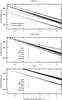 |
Fig. 10 Equilibrium temperatures of homogeneous spherical dust particles composed of different substances. |
The equilibrium temperature is found from the thermal balance equation 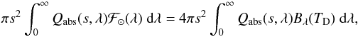 (1)where s is the radius of a spherical dust grain, λ the wavelength, ℱ⊙ the incident solar radiance flux, and Bλ(TD) the blackbody radiance at the dust particle’s temperature TD. The left-hand side provides the total energy absorbed from a mono-directional incident flux, and the right-hand side gives the total energy emitted, omni-directionally. We denote the absorption efficiency averaged over the solar spectrum with
  , and the same quantity averaged over a blackbody spectrum at temperature TD with
  , then by using the Stefan-Boltzmann law and the solar constant, Eq. (1) can be written in a more concise form (cf. Reach 1988):
 ![\begin{equation} \label{Reach Equ} T_\mathrm{D} = 279\;\mathrm{K}\; \left[\bar Q_\odot/\bar Q (T_\mathrm{D})\right]^{1/4} \left({\frac{R}{1\;\mbox{AU}}}\right)^{-1/2}, \end{equation}](/articles/aa/full_html/2015/12/aa25690-15/aa25690-15-eq87.png) (2)where R is the distance from the Sun. A perfect blackbody with Qabs = 1 throughout the spectrum has therefore a temperature of 279 K at 1 AU from the Sun, inversely proportional to the square root of the distance. This inverse-square-root trend is often closely followed by the real dust particles.
(2)where R is the distance from the Sun. A perfect blackbody with Qabs = 1 throughout the spectrum has therefore a temperature of 279 K at 1 AU from the Sun, inversely proportional to the square root of the distance. This inverse-square-root trend is often closely followed by the real dust particles.
The Kelsall model uses the temperature given by the equation 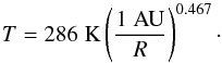 (3)Kelsall et al. (1998) emphasize that the dust temperature at 1 AU and absorption efficiencies could not be determined independently, so that the temperature was found by assuming the smooth cloud to be the dominant component with its spectrum in the mid-infrared being that of a pure blackbody (i.e., unit absorption efficiencies at λ = 4.9, 12, and 25 μm).
The equilibrium temperatures of dust particles are shown in Fig. 10 for a broad range of heliocentric distances. Temperatures used in the Kelsall model are plotted for comparison as well. Temperatures of the micrometer-sized particles clearly do not agree with Kelsall’s model, but they tend to be higher than temperatures of the larger particles of their composition as well. The reason is simple: their absorption efficiencies are too low at the wavelengths of ten and more micrometers, the size at which their larger counterparts emit the energy absorbed from the solar radiation flux, thus they warm to higher temperatures in order to shift the maximum of the Planck function to shorter wavelengths. Iron is an exception to this rule; all particles made of this substance are considerably warmer, being unable to emit the radiation thermally at longer wavelengths regardless of size. (It does not contradict the fact that communications in radiowaves are assisted by iron and other metallic antennas, as iron is very good at scattering the electromagnetic emission at longer wavelengths simultaneously.)
Amorphous carbonaceous particles (labeled “Zubko BE” in our plots) from ~ 10 μm in size are in the best agreement with the Kelsall model temperatures, among the real species considered here. This is a good indication for the Kelsall model, since most interplanetary meteoroids are indeed expected to be composed of carbonaceous material (Reach 1988; Dikarev et al. 2009). The temperatures of the silicaceous particles are somewhat lower, as olivine is rather transparent in the visual light that it absorbs, remaining opaque in the infrared light that it emits, but this difference is almost negligible starting from particle radii of 100 μm, especially at heliocentric distances beyond 1 AU (Fig. 11).
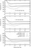 |
Fig. 11 Equilibrium temperatures of homogeneous spherical dust particles composed of different substances. |
In the following sections, however, we assume a single temperature for all dust particles of each substance, regardless of size. Our results are therefore less precise for dust particles smaller than ~ 100 μm in radii. Fortunately for the achievement of this paper’s goal, the microwave emission from large particles is more important for accurate predictions, since small particles are not efficient emitters at such long wavelengths.
4. Microwave thermal emission from dust
We are now ready to make maps of the thermal emission from the zodiacal dust for the broadest range of wavelengths and observation points. The surface brightness of the sky due to the zodiacal cloud, measured in units of power per unit solid angle and unit wavelength, observed from the location r in the direction specified by a unit vector  , is given by
 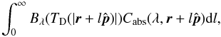 (4)where Cabs(λ,r) is the absorption cross-section of dust per unit volume of space. In the Kelsall model, Cabs is a sum of the products of the total cross-section area of dust by the emissivity modification factors for the wavelength λ, over all model components. Meteoroid engineering models require an evaluation of a nested integral over the particle size s,
  (5)where N(s,r) is the number density of meteoroids with radii greater than s at the location r. The minus sign in Eq. (5) is necessary since ∂N(s,r) /∂s ≤ 0. Figure 11 shows that the equilibrium temperature TD depends on particle size as well; however, this dependence is important only for small dust grains with s< 100 μm, which can be safely neglected in the microwaves.
We note that no color correction factor is applied, so that a difference of at least several percentage points is to be expected between our intensities and Kelsall’s zodiacal Atlas for the wavelengths where a direct comparison is possible.
4.1. All-sky maps
All-sky maps of the thermal emission from the interplanetary dust are made in Fig. 12 using the Kelsall model as well as meteoroid engineering models assuming that their particles are carbonaceous. Five observation wavebands of COBE, Planck, and WMAP are selected to demonstrate the transformation of the brightness distribution from the far infrared light (240 μm) to microwaves (13.6 mm).
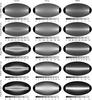 |
Fig. 12 All-sky maps of the thermal emission from the zodiacal cloud, according to the Kelsall model and two meteoroid engineering models (Divine 1993; Dikarev et al. 2005a) populated by the carbonaceous particles, as seen from Earth at the September equinox, for selected wavebands of the COBE, Planck, and WMAP observatories. The reference frame is ecliptic, the Mollweide projection is used, each map’s center points to the antisolar direction (i.e., the vernal equinox), a 30°-wide band around the Sun is masked. The grayscale of the upper row of maps is in MJy sterad-1, the other rows are in μK of a temperature in excess of the CMB. Each map has its own brightness scale. |
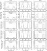 |
Fig. 13 Brightness profiles of the thermal emission from the zodiacal cloud along the great circles in the ecliptic plane (ecliptic latitude l = 0) and perpendicular to the ecliptic plane at solar elongation ε = 90°, according to the Kelsall model and two meteoroid engineering models populated by the carbonaceous particles, as seen from Earth, for selected wavebands of the COBE, Planck, and WMAP observatories. The excess temperatures are calculated with respect to the CMB. We note that the Kelsall model emissivity modification factors were normalized using the COBE and Planck data in the three upper rows, and the left column of plots may be the best representation of the observations available at these wavelengths. |
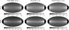 |
Fig. 14 All-sky maps of the thermal emission from the interplanetary dust predicted by two meteoroid engineering models, assuming that their constituent particles are composed of iron. The reference frame is as in Fig. 12. The brightness is provided in units of MJy sterad-1 for the COBE waveband centered at 240 μm, and in units of μK for the Planck and WMAP wavebands. |
At short wavelengths, emission from fine dust grains is dominant, and all models of the zodiacal cloud show the maximum emission near the Sun. The smooth background cloud is responsible for this brightness distribution in the Kelsall model, the core population in the Divine model, and the meteoroids with masses m< 10-5 g migrating toward the Sun under the Poynting-Robertson drag in IMEM are also concentrated near the Sun. As the wavelength grows, the fine dust grains fade out, but bigger meteoroids remain perceptible. The components of the Kelsall model possessing spectra of macroscopic particles, i.e., the asteroid dust bands, Divine’s asteroidal population, and the meteoroids with masses m> 10-5 g in IMEM are located mostly beyond the orbit of the Earth. Instead of the brightness peak of the fine dust at small solar elongations, the big meteoroids appear as a band, or bands, along the ecliptic, broadening in the antisolar direction: the surface brightness of diffuse objects does not depend on the distance from the observer, but their angular size increases owing to their proximity in the antisolar direction.
Figure 13 shows the brightness profiles built with the models from Fig. 12 for Earth-bound observatories scanning the celestial sphere in two important great circles, one in the ecliptic plane (zero ecliptic latitude) starting from the vernal equinox counterclockwise, and another perpendicular to the ecliptic plane, at the solar elongation of 90°, from the ecliptic north pole toward the apex of Earth’s motion about the Sun. The scan in the ecliptic plane is only unmasked, however, when the target area on the sky was visible with WMAP (solar elongations from 90° to 135°) or COBE DIRBE (solar elongations from 64° to 124°). We note that both profiles match at scan angles of 90° and 270° since the great circles cross there.
Figure 13 is especially interesting since it exhibits the Kelsall model under particular conditions, where it was fitted to the observations, in a number of plots. Indeed, the three upper rows of plots contain the brightness profiles at which the absorption efficiencies of model components were determined using the COBE DIRBE (Kelsall et al. 1998, λ = 240 μm) or Planck HFI data (Planck Collaboration XIV 2014, λ = 850 μm and 2.1 mm). The brightness profile along the scan in the ecliptic plane (dashed curve) at 240 μm was accessible to DIRBE almost entirely, as well as the entire scan perpendicular to the ecliptic plane (solid curve) at the same wavelength. The latter scan is just five degrees away from the Planck scans of the celestial sphere, and we used the absorption efficiencies found for the Kelsall model from the Planck data at 850 μm and 2.1 mm wavelengths. Thus, the Kelsall model predictions presented in these three plots may serve as the best representation of the observations available. This is unfortunately not applicable to the model predictions at other wavelengths nor is it necessarily true for all-sky maps, where the model can be extrapolated only. One must bear in mind that the absorption efficiencies for the Kelsall model components at the three wavelengths were determined with considerably high uncertainties, and the Planck data occasionally drove some of them negative. A direct comparison of any model considered in this paper with observations is beyond the scope of this paper since it requires a very extensive, dedicated effort (Kelsall et al. 1998; Planck Collaboration XIV 2014).
The Divine model and IMEM with the carbonaceous meteoroids appear to be substantially brighter than the Kelsall model. We note that IMEM was only fitted to the DIRBE data up to λ = 100 μm, using a composition of dust different from the triple used here, and Divine used no infrared data at all. Thus, no exact match with the Kelsall model is expected, especially at the wavelengths λ> 100 μm; Kelsall et al. (1998) themselves found the COBE DIRBE data at these wavelengths to insufficiently constrain the model (Sect. 2.1). The difference is substantially lower (25−30%) at shorter wavelengths (12−60 μm). Planck Collaboration XIV (2014) inferred the absorption efficiencies of the Kelsall model components for the Planck wavebands as well, and reported a lower emission from the zodiacal cloud than the Divine model and IMEM predict, as is shown in Figs. 12 and 13 on the plots for λ = 850 μm and 2.1 mm.
To pave the way for an explanation of the discrepancy, we note that the interplanetary dust is not entirely carbonaceous, and meteoroids of other chemical composition yield lower infrared and microwave thermal emission. In addition, meteoroid engineering models are fitted to many data sets, typically with an accuracy substantially lower than the models of the electromagnetic emission from dust. Finally, the fitting of the Kelsall model to the Planck data by Planck Collaboration XIV (2014) sometimes resulted in confusingly negative absorption efficiencies of dust, implying that the model may be incomplete, with some model components used by the fitting procedure to compensate for excessive emission from the other components. One can also see that the Kelsall model is deficient in the ecliptic plane, with the asteroid dust bands only allowed to shine just a little above and below that plane, and not in the ecliptic plane. A new fit to the Planck data using different meteoroid models would therefore be of great value, since these models may reproduce the relative brightness distribution of the microwave emission from dust more accurately, but they also may currently overestimate the number of big meteoroids in interplanetary space, so they also may be improved by such a fit.
Maps of the thermal emission of silicate particles are qualitatively similar to those of the carbonaceous meteoroids and are not shown here. However, the emission spectra of the zodiacal cloud for the silicate particles are discussed in the next section.
We make maps of the thermal emission from the iron meteoroids since they are remarkably different from the two materials discussed above (Fig. 14). Fine dust grains bulking near the Sun remain the brightest source regardless of the wavelength of observation. This stems from a very weak dependence of the absorption efficiency of iron particles on their size (within the range considered in this paper, see Fig. 9).
The difference in morphology of the maps for carbonaceous and iron particles suggests the way to discriminate between different sorts of interplanetary meteoroids from the microwave observations, when their accuracy permits.
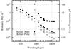 |
Fig. 15 Thermal emission spectra of the zodiacal cloud predicted by the Kelsall model for the apex of Earth’s motion about the Sun and ecliptic pole. Large squares are the excess temperatures w.r.t. the blackbody emission of the CMB (right scale), small squares are the absolute intensities of emission (left scale). |
4.2. Thermal emission spectra
Figures 15−17 show the thermal emission spectra of the zodiacal cloud predicted by Kelsall et al. pointed toward the apex of the Earth’s motion around the Sun and the ecliptic pole. The graphs are provided with two brightness scales: the absolute intensities are more natural and easier to read in the infrared wavelengths, whereas the excess temperatures are instantaneously comparable with other foreground emission sources in the CMB studies. The excess temperatures ΔT are defined as in Dikarev et al. (2009) so that Bλ(TCMB + ΔT) = Bλ(TCMB) + ϵ, where ϵ is the intensity of emission in excess of the CMB radiation at the temperature TCMB = 2.725 K, with the blackbody intensity Bλ being calculated precisely with the Planck formula rather than in the Rayleigh-Jeans approximation.
The Kelsall model is evaluated at the wavelengths of observations with COBE DIRBE and Planck HFI, for which the absorption efficiencies (“emissivity modification factors”) of the dust particles in the model components have been determined, and using the extrapolations described in Sect. 3.1 for the WMAP wavelengths. The model predicts rather low emission in the microwaves, for example, below 1 μK in the apex and below 0.1 μK in the ecliptic poles for λ> 3 mm. The emission in the apex is almost entirely due to the asteroid dust bands presumably having flat absorption efficiencies at these wavelengths, while a continuing decrease of the excess temperature with the wavelength increase for the polar line of sight for λ> 3 mm indicates that the smooth background cloud is contributing with Qabs ∝ λ-2. According to the Kelsall model, the foreground emission due to the zodiacal dust could indeed be disregarded in the WMAP survey of the microwave sky with its accuracy of 20 μK per 0.3° square pixel over one year.
The Divine model in Fig. 16 turns out to be much brighter, however.
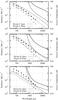 |
Fig. 16 Thermal emission spectra of the zodiacal cloud predicted by the Divine model for the apex of Earth’s motion around the Sun and the ecliptic pole, assuming that the dust particles are composed of amorphous carbon (top), silicate (middle), and iron (bottom) material. Thick curves are the excess temperatures with respect to the blackbody emission of the CMB (right scale), thin curves are the absolute intensities of emission (left scale). Also plotted are the absolute intensities of the Kelsall model for the wavelengths at which it was normalized to the observations (squares, see Fig. 15 for description). |
It predicts an excess temperature of up to ~ 20 μK in the WMAP W Band at λ = 3 mm, and ~ 5 μK in the K Band at λ = 13.6 mm, assuming that the meteoroids are all carbonaceous. Silicate meteoroids would add much less than 10 μK in the entire WMAP wavelength range. If the interplanetary dust particles were composed exclusively of iron, the Divine model would not let them shine brighter than the Kelsall model. Predictions made with IMEM for the same compositions are shown in Fig. 17. IMEM is dimmer than the Divine model, although it is still brighter than the Kelsall model.
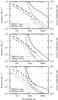 |
Fig. 17 Thermal emission spectra of the zodiacal cloud predicted by IMEM for the apex of Earth’s motion around the Sun and the ecliptic pole, assuming that the dust particles are composed of amorphous carbon (top), silicate (middle), and iron (bottom) material. Thick curves are the excess temperatures with respect to the blackbody emission of the CMB (right scale), thin curves are the absolute intensities of emission (left scale). Also plotted are the absolute intensities of the Kelsall model for the wavelengths at which it was normalized to the observations (squares, see Fig. 15 for description). |
We have also estimated the total mass and cross-section of meteoroids in the Divine model and IMEM within 5.2 AU from the Sun, i.e., inside a sphere considered by Kelsall et al. (1998) as the outer boundary of the zodiacal cloud. The Divine model contains ~ 2 × 10²⁰ g mass and 6 × 10⁻⁶ AU2 cross-section area of meteoroids. Assuming a density of 2.5 g cm-3, the total mass of meteoroids could be contained in a single spherical body of the radius ~ 30 km, the total cross-section area corresponds to a single sphere of radius ~ 2 × 10⁵ km; this radius would be possessed by a planet three times bigger than Jupiter. IMEM has only 6 × 10¹⁹ g mass and 6 × 10⁻⁶ AU2 cross-section area of meteoroids within 5.2 AU from the Sun.
Fixsen & Dwek (2002) assumed a certain size distribution of interplanetary meteoroids and used the optical properties for silicate, graphite, and amorphous carbonaceous particles in order to reproduce the annually averaged spectrum of the zodiacal cloud measured with the FIRAS instrument on board COBE. The smooth cloud of the Kelsall model was used to describe the spatial number density distribution of meteoroids. They found the total mass of meteoroids in the range 2−11 × 1018 g, i.e., remarkably lower than in the Divine model and IMEM.
5. Conclusion
We have made predictions of the microwave thermal emission from the zodiacal dust cloud in the wavelength range of COBE DIRBE, WMAP, and Planck observations. We used the Kelsall et al. (1998) model extrapolated to the microwaves using the optical properties of interplanetary dust inferred by Planck Collaboration XIV (2014) and Fixsen & Dwek (2002), and two meteoroid engineering models (Divine 1993; Dikarev et al. 2005a) in combination with the Mie light-scattering theory to simulate the thermal emission of silicate, carbonaceous, and iron spherical dust particles.
We have found that the meteoroid engineering models depict the thermal emission as substantially brighter and distributed differently across the sky and wavelengths than in the Kelsall model; this result is due to the presence of large populations of macroscopic particles in the meteoroid engineering models that are only available in the asteroid dust bands of the Kelsall model. The macroscopic particles (greater than ~ 100 μm in size) of the meteoroid engineering models do not get much brighter toward the Sun when viewed from near the Earth’s, since they are concentrated beyond Earth’s orbit, unlike smaller dust grains, to which the dominant component of the Kelsall model – the smooth cloud – can be safely attributed owing to its emission spectrum. The populations of macroscopic carbonaceous and silicate particles of the Divine model and IMEM are seen by an Earth-bound observer as bands along the ecliptic plane, broadening in the antisolar direction, keeping surface brightness approximately stable at zero ecliptic latitude (and excluding the smallest solar angles at which even a few particles can be exceptionally bright due to their high temperatures). The surface brightness predicted by the meteoroid engineering models appears analogously to that of Kelsall’s smooth cloud only if their particles are composed of iron, from our selection of materials, because of a very weak dependence of the absorption efficiency of iron particles on their size, so that small iron dust grains cannot be neglected with respect to their bigger counterparts even in the microwaves. However, iron is sufficiently dim in both the IR and microwaves.
The macroscopic particles in Kelsall’s asteroid dust bands are revealed as twin brightness enhancements above and below the ecliptic plane, whereas the meteoroid engineering models are characterized by a single enhancement nearly along that plane, with local maxima along the asteroid belt latitudes only in IMEM. This difference might explain the difficulties in fitting the Kelsall model to the Planck observations at the wavelengths of its High Frequency Instrument, including the unphysical negative absorption efficiencies found by Planck Collaboration XIV (2014) for some components of the Kelsall model, as well as their uncertainty that can reach and even exceed the best-fit value.
Both the Divine model and IMEM confirm an earlier estimate of a ~ 10 μK thermal emission from interplanetary dust (Dikarev et al. 2009) for the WMAP observations, provided that the dominant particle composition is carbonaceous. This is well above the systematic biases accounted for in this mission’s data and, to an even higher degree, in the much more sensitive survey performed with Planck, for which the Kelsall model might be insufficient, if not improper. A detailed analysis of implications of a more intensive thermal emission from interplanetary dust for the cosmological studies is beyond the scope of this work. However, some important issues can already be highlighted.
We observe that the interplanetary dust emission comes from a band on the sky that is parity symmetric and thus we would expect that even multipole moments (including the monopole) are mainly affected. These might lead to corrections to the even low-ℓ multipole moments in a way that is comparable to other effects like the Doppler quadrupole (Schwarz et al. 2004; Notari & Quartin 2015).
As the thermal emission from the considered models of interplanetary dust is smooth along the ecliptic, we do not expect sizable contributions to high-ℓ multipole moments. This might suggest that the interplanetary dust could explain some of the large-angle anomalies of the CMB (Copi et al. 2015a,b; Planck Collaboration XXIII 2014); however, the way in which the quadrupole and octopole are aligned with each other and with the dipole does not seem to be obviously linked to the expected pattern (Dikarev et al. 2008). On the other hand, a modification of the quadrupole and other low-ℓ multipoles will change the statistical significance of the low-ℓ anomalies.
A more detailed search for and account of interplanetary dust are therefore worthwhile in the CMB experiment results. Maps of the microwave sky should also be scrutinized to constrain the number of macroscopic particles in the meteoroid engineering models as they are important in order to assess and mitigate successfully the impact hazard for long-term manned missions with large spaceships to the Moon or Mars.
Acknowledgments
The authors thank Carlo Burigano, Craig Copi, Kenneth Ganga, Dragan Huterer, Pavel Naselsky and Glenn Starkman for insightful discussions. Thanks are also due to Helenka Kinnan for valuable linguistic corrections. This work was supported by the German Research Foundation (Deutsche Forschungsgemeinschaft), grant reference SCHW 1344/3 – 1, and via the Research Training Group 1620 “Models of Gravity”.
References
- Babich, D., Blake, C. H., & Steinhardt, C. L. 2007, ApJ, 669, 1406 [NASA ADS] [CrossRef] [Google Scholar]
- Bennett, C. L., Hill, R. S., Hinshaw, G., et al. 2011, ApJS, 192, 17 [NASA ADS] [CrossRef] [Google Scholar]
- Bennett, C. L., Larson, D., Weiland, J. L., et al. 2013, ApJS, 208, 20 [Google Scholar]
- Bohren, C. F., & Huffman, D. R. 1983, Absorption and scattering of light by small particles (New York: Wiley) [Google Scholar]
- Copi, C. J., Huterer, D., Schwarz, D. J., & Starkman, G. D. 2010, Adv. Astron., 2010, 92 [Google Scholar]
- Copi, C. J., Huterer, D., Schwarz, D. J., & Starkman, G. D. 2015a, MNRAS, 451, 2978 [NASA ADS] [CrossRef] [Google Scholar]
- Copi, C. J., Huterer, D., Schwarz, D. J., & Starkman, G. D. 2015b, MNRAS, 449, 3458 [NASA ADS] [CrossRef] [Google Scholar]
- Dermott, S. F., Nicholson, P. D., Burns, J. A., & Houck, J. R. 1984, Nature, 312, 505 [NASA ADS] [CrossRef] [Google Scholar]
- Dikarev, V., & Grün, E. 2004, in Order and Chaos in Stellar and Planetary Systems, Proc. Conf. held 17–24 August, 2003 at St. Petersburg State University, Russia, eds. G. G. Byrd, K. V. Kholshevnikov, A. A. Myllri, I. I. Nikiforov, & V. V. Orlov (San Francisco: ASP) ASP Conf. Proc., 316 [Google Scholar]
- Dikarev, V., Grün, E., Baggaley, J., et al. 2004, Earth Moon Planets, 95, 109 [NASA ADS] [CrossRef] [Google Scholar]
- Dikarev, V., Grün, E., Baggaley, J., et al. 2005a, Advances in Space Res., 35, 1282 [Google Scholar]
- Dikarev, V., Grün, E., Landgraf, M., & Jehn, R. 2005b, in 4th European Conf. on Space Debris, ed. D. Danesy, ESA SP, 587, 271 [NASA ADS] [Google Scholar]
- Dikarev, V., Preuß, O., Solanki, S., Krüger, H., & Krivov, A. 2008, Earth Moon Planets, 102, 555 [NASA ADS] [CrossRef] [Google Scholar]
- Dikarev, V., Preuß, O., Solanki, S., Krüger, H., & Krivov, A. 2009, ApJ, 705, 670 [NASA ADS] [CrossRef] [Google Scholar]
- Divine, N. 1993, J. Geophys. Res., 98, 17029 [NASA ADS] [CrossRef] [Google Scholar]
- Drolshagen, G., Dikarev, V., Landgraf, M., Krag, H., & Kuiper, W. 2008, Earth Moon Planets, 102, 191 [NASA ADS] [CrossRef] [Google Scholar]
- Fixsen, D. J., & Dwek, E. 2002, ApJ, 578, 1009 [NASA ADS] [CrossRef] [Google Scholar]
- Galligan, D. P., & Baggaley, W. J. 2004, MNRAS, 353, 422 [NASA ADS] [CrossRef] [Google Scholar]
- Gor’kavyi, N. N., Ozernoy, L. M., Mather, J. C., & Taidakova, T. 1997, ApJ, 488, 268 [NASA ADS] [CrossRef] [Google Scholar]
- Grün, E., & Dikarev, V. 2009, Landolt-Börnstein Numerical Data and Functional Relationships in Science and Technology, Group IV, Vol. 4B, 501 [Google Scholar]
- Grün, E., Zook, H. A., Fechtig, H., & Giese, R. H. 1985, Icarus, 62, 244 [NASA ADS] [CrossRef] [Google Scholar]
- Grün, E., Staubach, P., Baguhl, M., et al. 1997, Icarus, 129, 270 [NASA ADS] [CrossRef] [Google Scholar]
- Hansen, M., Kim, J., Frejsel, A. M., et al. 2012, J. Cosmol. Astropart. Phys., 10, 59 [NASA ADS] [CrossRef] [Google Scholar]
- Kelsall, T., Weiland, J. L., Franz, B. A., et al. 1998, ApJ, 508, 44 [NASA ADS] [CrossRef] [Google Scholar]
- Leinert, C., Roser, S., & Buitrago, J. 1983, A&A, 118, 345 [NASA ADS] [Google Scholar]
- Low, F. J., Young, E., Beintema, D. A., et al. 1984, ApJ, 278, L19 [NASA ADS] [CrossRef] [Google Scholar]
- Maris, M., Burigana, C., & Fogliani, S. 2006, A&A, 452, 685 [NASA ADS] [CrossRef] [EDP Sciences] [Google Scholar]
- McNamara, H., Jones, J., Kauffman, B., et al. 2004, Earth Moon Planets, 95, 123 [NASA ADS] [CrossRef] [Google Scholar]
- Notari, A., & Quartin, M. 2015, J. Cosmol. Astropart. Phys., 06, 047 [Google Scholar]
- Planck Collaboration I. 2014, A&A, 571, A1 [NASA ADS] [CrossRef] [EDP Sciences] [Google Scholar]
- Planck Collaboration XIV. 2014, A&A, 571, A14 [NASA ADS] [CrossRef] [EDP Sciences] [Google Scholar]
- Planck Collaboration XXIII. 2014, A&A, 571, A23 [NASA ADS] [CrossRef] [EDP Sciences] [MathSciNet] [PubMed] [Google Scholar]
- Pollack, J. B., Hollenbach, D., Beckwith, S., et al. 1994, ApJ, 421, 615 [NASA ADS] [CrossRef] [Google Scholar]
- Reach, W. T. 1988, ApJ, 335, 468 [NASA ADS] [CrossRef] [Google Scholar]
- Reach, W. T. 1992, ApJ, 392, 289 [NASA ADS] [CrossRef] [Google Scholar]
- Schlegel, D. J., Finkbeiner, D. P., & Davis, M. 1998, ApJ, 500, 525 [NASA ADS] [CrossRef] [Google Scholar]
- Schwarz, D. J., Starkman, G. D., Huterer, D., & Copi, C. J. 2004, Phys. Rev. Lett., 93, 221301 [NASA ADS] [CrossRef] [PubMed] [Google Scholar]
- Staubach, P., Grün, E., & Jehn, R. 1997, Adv. Space Res., 19, 301 [NASA ADS] [CrossRef] [Google Scholar]
- Zubko, V. G., Krelowski, J., & Wegner, W. 1996, MNRAS, 283, 577 [NASA ADS] [CrossRef] [Google Scholar]
Appendix A: Frequencies and wavelengths of selected CIB and CMB observatories
Table A.1 provides quick conversions between frequencies and wavelengths for the observation wavebands of infrared detectors and radiometers.
Frequencies ν, wavelengths λ, and bandwidths Δν/ν of the CIB/CMB observations with COBE DIRBE wavelength bands 4 through 10, WMAP, and Planck.
All Tables
Frequencies ν, wavelengths λ, and bandwidths Δν/ν of the CIB/CMB observations with COBE DIRBE wavelength bands 4 through 10, WMAP, and Planck.
All Figures
|
Fig. 1 Profiles of particle cross-section area density predicted with selected meteoroid models and compared with each other: ecliptic radial (left) and latitudinal at 1 AU from the Sun (right, the vernal equinox is at latitude 0°). |
| In the text | |
|
Fig. 2 Radial and latitudinal profiles of particle cross-section area density in the Kelsall model, component by component. |
| In the text | |
|
Fig. 3 Radial and latitudinal profiles of particle cross-section area density in the Divine model, component by component. |
| In the text | |
|
Fig. 4 Radial and latitudinal profiles of particle cross-section area density in IMEM, component by component. The density plots are not smooth since the orbital distributions in IMEM are approximated by step functions. |
| In the text | |
|
Fig. 5 Cumulative mass distribution of interplanetary meteoroids (Grün et al. 1985, top); meteoroid lifetimes against mutual collisions and Poynting-Robertson drag (middle); and cumulative mass distributions of meteoroid populations in IMEM (Dikarev et al. 2005a, bottom) including the interstellar dust, which is ignored in this paper owing to the tiny sizes of the constituent particles. The flux of meteoroids with m> 10-5 g is lower in IMEM than in the Grün model since the impact velocities of big meteoroids are higher at 1 AU from the Sun in IMEM and they produce larger craters on the lunar rocks than in the Grün model, which assumed a single impact velocity for all meteoroid sizes. |
| In the text | |
|
Fig. 6 Cumulative distribution functions of particle cross-section area in mass (size) for each population of the interplanetary meteoroid model by Divine (1993) and IMEM (Dikarev et al. 2005a). The material density of particles is equal to 2.5 g cm-3 in both models except Divine’s eccentric population where it is ten times lower. The particle size scale should not be used in combination with the plot for the latter population. |
| In the text | |
|
Fig. 7 Particle cross-section area densities (per unit volume of space, AU2/AU3) for each component or population of the meteoroid models by Kelsall et al. (1998), Divine (1993), and IMEM (Dikarev et al. 2005a). We note that two maps for the cometary dust in IMEM are plotted in a different scale. |
| In the text | |
|
Fig. 8 Absorption efficiencies (“emissivity modification factors”, see text for explanation) of dust in the Kelsall model determined for the COBE DIRBE wavelengths by Kelsall et al. (1998), gray area on the plot, and for the Planck HFI wavelengths by Planck Collaboration XIV (2014). Fixsen & Dwek (2002) have also used the data from the COBE FIRAS instrument to determine the annually averaged spectrum of the zodiacal cloud plotted here with a dotted line. |
| In the text | |
|
Fig. 9 Optical constants and absorption efficiencies for olivine and iron of Pollack et al. (1994), and for amorphous carbonaceous grains from the “BE” sample of Zubko et al. (1996) used in this paper, in addition to the data introduced by Dikarev et al. (2009). The absorption efficiencies are calculated for the sizes of spherical dust grains indicated in the bottom row of plots. |
| In the text | |
|
Fig. 10 Equilibrium temperatures of homogeneous spherical dust particles composed of different substances. |
| In the text | |
|
Fig. 11 Equilibrium temperatures of homogeneous spherical dust particles composed of different substances. |
| In the text | |
|
Fig. 12 All-sky maps of the thermal emission from the zodiacal cloud, according to the Kelsall model and two meteoroid engineering models (Divine 1993; Dikarev et al. 2005a) populated by the carbonaceous particles, as seen from Earth at the September equinox, for selected wavebands of the COBE, Planck, and WMAP observatories. The reference frame is ecliptic, the Mollweide projection is used, each map’s center points to the antisolar direction (i.e., the vernal equinox), a 30°-wide band around the Sun is masked. The grayscale of the upper row of maps is in MJy sterad-1, the other rows are in μK of a temperature in excess of the CMB. Each map has its own brightness scale. |
| In the text | |
|
Fig. 13 Brightness profiles of the thermal emission from the zodiacal cloud along the great circles in the ecliptic plane (ecliptic latitude l = 0) and perpendicular to the ecliptic plane at solar elongation ε = 90°, according to the Kelsall model and two meteoroid engineering models populated by the carbonaceous particles, as seen from Earth, for selected wavebands of the COBE, Planck, and WMAP observatories. The excess temperatures are calculated with respect to the CMB. We note that the Kelsall model emissivity modification factors were normalized using the COBE and Planck data in the three upper rows, and the left column of plots may be the best representation of the observations available at these wavelengths. |
| In the text | |
|
Fig. 14 All-sky maps of the thermal emission from the interplanetary dust predicted by two meteoroid engineering models, assuming that their constituent particles are composed of iron. The reference frame is as in Fig. 12. The brightness is provided in units of MJy sterad-1 for the COBE waveband centered at 240 μm, and in units of μK for the Planck and WMAP wavebands. |
| In the text | |
|
Fig. 15 Thermal emission spectra of the zodiacal cloud predicted by the Kelsall model for the apex of Earth’s motion about the Sun and ecliptic pole. Large squares are the excess temperatures w.r.t. the blackbody emission of the CMB (right scale), small squares are the absolute intensities of emission (left scale). |
| In the text | |
|
Fig. 16 Thermal emission spectra of the zodiacal cloud predicted by the Divine model for the apex of Earth’s motion around the Sun and the ecliptic pole, assuming that the dust particles are composed of amorphous carbon (top), silicate (middle), and iron (bottom) material. Thick curves are the excess temperatures with respect to the blackbody emission of the CMB (right scale), thin curves are the absolute intensities of emission (left scale). Also plotted are the absolute intensities of the Kelsall model for the wavelengths at which it was normalized to the observations (squares, see Fig. 15 for description). |
| In the text | |
|
Fig. 17 Thermal emission spectra of the zodiacal cloud predicted by IMEM for the apex of Earth’s motion around the Sun and the ecliptic pole, assuming that the dust particles are composed of amorphous carbon (top), silicate (middle), and iron (bottom) material. Thick curves are the excess temperatures with respect to the blackbody emission of the CMB (right scale), thin curves are the absolute intensities of emission (left scale). Also plotted are the absolute intensities of the Kelsall model for the wavelengths at which it was normalized to the observations (squares, see Fig. 15 for description). |
| In the text | |
Current usage metrics show cumulative count of Article Views (full-text article views including HTML views, PDF and ePub downloads, according to the available data) and Abstracts Views on Vision4Press platform.
Data correspond to usage on the plateform after 2015. The current usage metrics is available 48-96 hours after online publication and is updated daily on week days.
Initial download of the metrics may take a while.