| Issue |
A&A
Volume 584, December 2015
|
|
|---|---|---|
| Article Number | A6 | |
| Number of page(s) | 11 | |
| Section | The Sun | |
| DOI | https://doi.org/10.1051/0004-6361/201425348 | |
| Published online | 13 November 2015 | |
Determining energy balance in the flaring chromosphere from oxygen V line ratios
SUPA School of Physics and Astronomy, University of Glasgow, Glasgow G12 8QQ, UK
e-mail: This email address is being protected from spambots. You need JavaScript enabled to view it.
Received: 17 November 2014
Accepted: 14 September 2015
Abstract
Context. The impulsive phase of solar flares is a time of rapid energy deposition and heating in the lower solar atmosphere, leading to changes in the temperature and density structure of the region.
Aims. We use an O v density diagnostic formed from the λ192 /λ248 line ratio, provided by the Hinode/EIS instrument, to determine the density of flare footpoint plasma at O v formation temperatures of ~2.5 × 10⁵ K, giving a constraint on the properties of the heated transition region.
Methods. Hinode/EIS rasters from 2 small flare events in December 2007 were used. Raster images were co-aligned to identify and establish the footpoint pixels, multiple-component Gaussian line fitting of the spectra was carried out to isolate the density diagnostic pair, and the density was calculated for several footpoint areas. The assumptions of equilibrium ionisation and optically-thin radiation for the O v lines used were assessed and found to be acceptable. For one of the events, properties of the electron distribution were deduced from earlier RHESSI hard X-ray observations. These were used to calculate the plasma heating rate delivered by an electron beam for 2 semi-empirical atmospheres under collisional thick-target assumptions. The radiative loss rate for this plasma was also calculated for comparison with possible energy input mechanisms.
Results. Electron number densities of up to 1011.9 cm-3 were measured during the flare impulsive phase using the O v λ192 /λ248 diagnostic ratio. The heating rate delivered by an electron beam was found to exceed the radiative losses at this density, corresponding to a height of 450 km, and when assuming a completely ionised target atmosphere far exceed the losses but at a height of 1450–1600 km. A chromospheric thickness of 70–700 km was found to be required to balance a conductive input to the O v-emitting region with radiative losses.
Conclusions. Electron densities have been observed in footpoint sources at transition region temperatures, comparable to previous results but with improved spatial information. The observed densities can be explained by heating of the chromosphere by collisional electrons, with O v formed at heights of 450–1600 km above the photosphere, depending on the atmospheric ionisation fraction.
Key words: Sun: atmosphere / Sun: chromosphere / Sun: flares / Sun: transition region / Sun: X-rays, gamma rays / Sun: UV radiation
Current address: INAF–Osservatorio Astrofisico di Arcetri, 50125 Firenze, Italy.
© ESO, 2015
1. Introduction
Solar flares are the result of a sudden reconfiguration of the active region magnetic field, releasing of the order of 1031 ergs of energy (for a medium-sized event) in a matter of minutes. They are visible across the electromagnetic spectrum, but particularly in the dramatic appearance of high temperature extreme ultraviolet (EUV) and soft X-ray (SXR) emitting plasmas. The maximum intensity from the EUV and SXR plasmas occur roughly coincident with, or lag slightly behind, an abrupt hard X-ray (HXR) burst emitted by electrons that have been accelerated to non-thermal energies and lose energy via bremsstrahlung radiation in a dense, collisional plasma. HXR imaging spectroscopy by the Reuven Ramaty High Energy Solar Spectroscopic Imager (RHESSI; Lin et al. 2002) has successfully shown that this emission is mainly confined to compact footpoint regions in the low solar atmosphere – chromosphere to low-corona – and in some cases dense loop sources. The energy collisionally deposited in the chromosphere by electron-electron and electron-ion collisions is capable of explaining rapid heating of footpoint plasma, to millions of kelvin. Theoretical models of collisional energy deposition and the response of the atmosphere have a long heritage and are now very detailed in terms of their treatment of dynamics and radiation transfer (e.g. Nagai & Emslie 1984; Allred et al. 2005; Liu et al. 2009); observational constraints are of course needed to test whether the models are adequate.
How these electrons are accelerated out of an initially (almost) thermal distribution remains a mystery, and decades of effort have focused on using observational signatures to try to understand this. This is not straightforward: observational signatures, other than those directly produced by the accelerated electrons themselves (i.e. HXR and gyrosynchrotron radiation) tend to say more about the heated medium than about the energetic particles that heat it, though direct collisional effects from non-thermal particles may be detectable from detailed examination of spectral features (e.g. Kulinová et al. 2011). However, the distribution of density and temperature in the flare-heated atmosphere, as a function of time, bears some relation to the distribution in space and time of the heating, and thus to the distribution of non-thermal particles which are thought responsible for the collisional heating. The standard collisional thick-target model for the heating of the flare atmosphere invokes collisional loss by non-thermal electrons (remote from their acceleration location) and efforts to model the flare atmospheric response have tended to focus on this.
Theoretical problems with this model, primarily the large beam number density required by observations and the associated difficulties with the beam propagating stably, have led to alternatives being proposed to the collisional thick-target model, such as local acceleration or re-acceleration of electrons in the chromosphere (Fletcher & Hudson 2008; Brown et al. 2009), while flare heating of the chromosphere by wave dissipation Russell & Fletcher (2013) or by thermal conduction (Graham et al. 2013) have also been suggested. None of these proposed mechanisms have been implemented into atmospheric modelling so far, or their radiation signatures evaluated.
Flare energy deposition leads to rapid heating and ionisation of compact regions of the lower solar atmosphere to nearly 10 MK (e.g. Mrozek & Tomczak 2004; Fletcher et al. 2013; Graham et al. 2013) and expansion of the local plasma, known as chromospheric evaporation, observed spectroscopically in the EUV and SXR (e.g. Antonucci & Dennis 1983; Czaykowska et al. 1999; Milligan & Dennis 2009). The resulting flaring solar atmosphere is strongly stratified in density and temperature, and we need observations to completely specify its properties over a broad range of temperatures. Interpreting the atmospheric structure from optically thin observations of footpoint radiation is extremely challenging because height information cannot be directly extracted. We can however measure the density at specific temperatures and compare these to the structure of a modelled pre-flare or flaring atmospheres. In this paper we focus on the properties of plasma at a temperature of 2.5 × 10⁵ K (log T = 5.4) using a density sensitive O v ratio λ192 /λ248.
Previous work with Hinode/EIS has identified flare footpoint densities of a few times 1010 to 1011 cm-3 (Watanabe et al. 2010; Del Zanna et al. 2011; Graham et al. 2011) at temperatures of 1–2 MK, but higher densities were documented in the late 70 s and early 80 s using the Skylab NRL normal incidence slit spectrograph S082B (Bartoe et al. 1977) and the Ultraviolet Spectrometer and Polarimeter (UVSP) instrument on board the Solar Maximum Mission (SMM; Woodgate et al. 1980). Doschek et al. (1977) and Feldman et al. (1977) derived flare densities from O iv ratios at 105 K from Skylab slit data. The spectral profiles had distinct velocity-shifted components with densities of 1011 and 1012 cm-3 in the stationary, and at least 1013 cm-3 in the downward-moving component. At similar line formation temperatures Cheng et al. (1982) used the O iv 1401 Å to Si iv 1402.7 Å ratio and found that a pre-flare density of 2.5 × 1011 cm-3 rose to 3 × 1012 cm-3 during the flare impulsive phase. This enhancement was also located within a footpoint kernel and coincided temporally with a HXR burst. The limited spatial resolution in these instruments did, however, make the distinction between loop and footpoint sources difficult.
In this paper we make new measurements of flare footpoint densities at transition region temperatures, finding similar enhanced densities, although addressing the earlier ambiguity in identifying the emitting region by employing the capabilities offered by Hinode/EIS. Section 2 introduces the data and spectral fitting of the diagnostic lines, Sect. 3 reveals the measured footpoint densities, Sect. 4 considers the validity of the assumption of optically thin plasma in ionisation equilibrium, and finally Sects. 5 and 6 interpret the results within the framework of an atmosphere heated collisionally by electrons and one heated solely by a conductive flux.
2. Hinode/EIS data
Good diagnostics of density below log T = 6.0 are uncommon in the EIS spectral range and, as far as we are aware, have not been used in the study of flare footpoint plasmas. Transition region lines during the flare impulsive phase are observed to rise almost simultaneously with the HXR response (Poland et al. 1984; Mariska & Poland 1985) and density measurements of the emitting plasma at these temperatures are therefore extremely useful to help locate the heated plasma within the atmosphere in relation to the HXR emission. The O v n = 3 transitions at 192.904 Å and 248.460 Å are observed by Hinode/EIS and their ratio forms a diagnostic pair sensitive to densities up to around 1012 cm-3 (Widing et al. 1982). A formation temperature at equilibrium of 250 000 K places their maximum emission within the transition region in the quiet-sun (Vernazza et al. 1981) and the diagnostic curve is shown in Fig. 1.
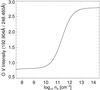 |
Fig. 1 Diagnostic ratio for O v 192.904 Å/248.460 Å. |
In this article we analyse data from these lines during the impulsive phases of two C-class flares; SOL2007-12-14T01:39 (Flare 1) and SOL2007-12-14T14:16 (Flare 2). The flares have been the subject of previous papers; in an emission measure analysis (Graham et al. 2013), and evaporation and non-thermal broadening study (Milligan & Dennis 2009; Milligan 2011) respectively.
The impulsive phase in each flare was mostly captured in one raster scan by EIS and the raster closest to the GOES SXR derivative peak was chosen to best represent the time of maximum energy deposition (see Graham et al. 2013). RHESSI coverage was not available for Flare 1, but the presence of non-thermal RHESSI HXR footpoints was confirmed for Flare 2 (Milligan & Dennis 2009). Footpoints were identified in both flares by the sudden appearance of compact enhancements in the cooler EIS lines, e.g. He ii and Fe viii at log T = 4.5–5.7, explained by a rise in the chromospheric temperature, and enhanced electron densities in the Fe xii – xiv diagnostics at temperatures between log T = 6.1–6.3 (Milligan 2011), again a sign that the dense lower atmosphere is being heated (Graham et al. 2011). Again we refer the reader to the previous work in Graham et al. (2013) for more details on the raster selection and footpoint identification.
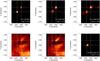 |
Fig. 2 Fitted intensities in several different temperature lines for the 01:35:28 UT raster (Flare 1) after correcting for the EIS detector offset. White dotted lines show the position of the footpoints in each image relative to the O v 192 Å line. The x-offset is highlighted by the black strip on the left of the Fe xiv 274 Å image. |
Both flares used the same CAM_ARTB_RHESSI_b_2 study having an exposure time of 10 s using the 2′′ slit covering a 40″ × 144″ area. The slit stepping for these rasters was continuous, not sparse, in the x direction, advantageous in these smaller events, and crossed the footpoints during the impulsive phase. The rasters were prepared with the standard SolarSoft eis_prep routine.
Time and wavelength dependent changes in the absolute calibration of both the EIS spectrograph detectors were recently re-characterised by Del Zanna (2013) and Warren et al. (2014), finding that both detectors are degrading at independent rates; this complicates the O v diagnostic as the lines fall on separate detectors (see next section). The data in our study is from relatively early in the Hinode mission, yet the new calibrations vary significantly from the pre-flight set. For our analysis we use the Warren et al. (2014) calibration by applying the eis_recalibrate_intensity.pro routine.
2.1. EIS image alignment
The diagnostic lines in question occur on the two different CCDs of the EIS spectrograph, which are not identically aligned with respect to the grating. This introduces a fixed spatial offset in the slit direction (y-axis) between features observed on each CCD. In addition, the short wavelength CCD is tilted slightly relative to the grating, creating a further wavelength-dependent offset (longer wavelengths appearing lower on the CCD). In the case of a diagnostic ratio it is extremely important to remove these effects to ensure that we observe the same feature in both wavelengths. The tilt was characterised by Young et al. (2009) and a correction included in the eis_ccd_offset.pro routine which returns the y-offset required to correct both the grating tilt and spatial offset.
We also performed our own cross-correlation using the Fe xiii 202 Å and Fe xiv 274 Å lines for a range of binary thresholds. We found an average shift of 16.7′′ in the y-axis (slit axis) but also a shift of 1 pixel, or 2.0′′, in the x-axis. Our y-offset was comparable with the 17.06′′ shift given by the eis_ccd_offset routine, affirming the Young et al. (2009) prediction. The additional 2′′x-offset was also documented by Young et al. (2007) and later attributed to an optics focusing effect; mostly corrected for in 24 August 2008. The only complication with alignment in the x-direction is that the same feature is seen in two consecutive slit steps, and correcting for it effectively halves the observing cadence.
In Fig. 2 we show example fitted intensity images in several emission lines from the Flare 1 raster after correlation. Here we use our measured x-shift while using the wavelength dependent y-offset calculated by the EIS routine. The white dotted lines cross the same (x,y) location in each image, centred on the footpoints in O v 192 Å, and intersect the corresponding bright emission in all lines for the northern footpoint. The southern footpoint has an anomalous x-shift of around 2′′ when observed at some wavelengths, which is curious as the shift is not apparent in its northern companion, ruling out a problem with the correlation. It is also not temperature sensitive, as both Fe xxiii and O v are equally offset while the He ii 256 Å image shows no change. The offset is puzzling as an instrumental effect would be expected to alter the other footpoint’s position, yet there is no obvious relation to the line temperature or wavelength. We cannot discount the effects of optical depth here, as the active region lies at 450′′ on the solar disc with a 29 deg projection to Earth. A small filament seen in TRACE images (not shown here) lies just to the north of the footpoint, perhaps absorbing some emission from lines with a higher opacity. We discuss the opacity in Sect. 4.
2.2. Line fitting technique
Multiple component Gaussian fits with several constraints are required to extract the diagnostic line intensities. The oxygen 248 Å line is relatively unblended but the density-sensitive 192 Å transition lies in a challenging part of the EIS spectral range. Several oxygen and iron lines formed at different temperatures lie in close proximity and interpreting their individual intensities is difficult, or sometimes impossible without constraints from other lines in the raster. Significant contributions, as predicted by the CHIANTI v7.1.3 atomic database (Dere et al. 1997; Landi et al. 2013), are listed in Table 1.
192 Å – The target 192.904 Å line lies in a complex profile of six O v lines, two coronal Fe xi lines, and a hot Ca xvii line; including a linear background makes a total of 29 free parameters. In order to reduce the required number of free parameters we use a fitting routine based on the technique described in Ko et al. (2009). The neighbouring five O v lines are first constrained by fixing their intensities, centroids, and line widths relative to the target 192.904 Å fit. The intensity ratios are estimated from CHIANTI for an electron density of 1012 cm-3 and are shown in Table 1. There is some density sensitivity among the other oxygen lines relative to 192.904 Å, plotted in Fig. 3, however only the 192.797 Å line has any significant density sensitivity, and only up to 1012 cm-3. As we do not know the density before fitting we have tested that the choice of density will have a minimal effect. Changing the density from 1012 to 1010 cm-3 raises the fitted 192.904 Å intensity by <10%. By using the higher density of 1012 cm-3 it serves to reduce the diagnostic ratio, erring on the side of a lower density estimate.
Fe xi 192.627 Å is distinct from the overall profile and can be fitted with little constraint, only requiring that the width be ± 40% of the well-observed Fe xi 188.230 Å line. Fe xi 192.814 Å is tied to the Fe xi 188.230 Å line by a constant intensity ratio of 0.2, which is insensitive to density. The centroid shift of both iron lines within the profile were also tied to the 188 Å line. Finally, the parameters of the last remaining Ca xvii line are left mostly unconstrained, with the only limit imposed being that the centroid position should not be red-shifted.
248 Å – The 248 Å O v line is more straightforward to fit as the Ar xiii contribution is in most cases resolvable. Al viii however, lies near the O v line centroid and some extra constraint is needed. From CHIANTI, using the DEM derived in Graham et al. (2013), the Al viii contribution is 10% of the O v intensity for photospheric abundances.
Emission lines within the 192 Å and 248 Å profiles.
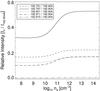 |
Fig. 3 Density sensitivity of the blended O v lines with respect to the 192.904 Å transition. |
2.3. Footpoint pixel selection
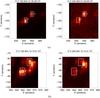 |
Fig. 4 Intensity maps for both 192.904 Å and 248.460 Å lines corresponding to the impulsive phase for both flares. Two footpoints regions (1 and 2) are bounded in each flare by a white box (pixels under the line are included in the selection). The brightest pixel within each footpoint region is also identified by a black cross. |
In Fig. 4 we show the intensity maps in the 192.904 Å and 248.460 Å lines (left and right columns) for each flare (rows (a) and (b)). The compact footpoints are clearly identified against the background active region emission. In each flare two footpoint regions are defined by 6″ × 7″ white boxes; including all of the pixels within and under the white lines. The brightest 192 Å pixel in each footpoint region is marked by a black cross on both wavelengths. We noted that the brightest emission in both 192 Å and 248 Å lines did not always coincide. This is particularly clear in Flare 1 (Fig. 4a), where for Footpoint 1 the strongest emission in 248 Å is found one pixel (2′′) to the right of 192 Å (discussed in the previous section).
To acknowledge these small position uncertainties the intensity ratio is calculated using two methods. In the first method, spectra for each footpoint are averaged over the region within the white box, which is the same for both lines, before fitting and finding the ratio. The second method takes the ratio from the pixel brightest in 192 Å within the footpoint regions and makes the ratio with same pixel in 248 Å; plus a binning by ±1 pixels in the y-direction (a 2″ × 3″ region) to account for any correlation uncertainty. Densities from the box method are likely to return a lower limit on the density as it includes pixels from outside of the footpoint regions. The latter “pixel” method assumes that the brightest emission originates from the same source in both lines but has enough spread to account for uncertainties in the correlation. Of course if the source size is smaller than the instrumental point spread function (3–4′′ in EIS) then the density in unresolved structures may yet be higher.
3. Results
3.1. Fitted spectra
The fitted spectra for the bright pixels in Fig. 5 (Flare 1) show a clear enhancement of the O v 192 Å line (red line, right hand profiles) compared to the pre-flare (Fig. 7) with the line being distinct from the rest of the profile. This 192.904 Å transition is excited from a metastable level and is expected to brighten quickly as the dense emitting plasma is heated; similar line profiles in transition region brightenings were also found by Young et al. (2007). The unconstrained Ca xvii emission (blue line) in these footpoints makes a small contribution among the other predicted Fe xi and O v intensities (green dashed and black dotted lines respectively). In Fig. 6 the Ca xvii (blue line) emission is more significant, possibly due to more hot loop material being present along the line of sight.
We have highlighted the spectra partly to demonstrate the robustness of the fitting method. Between the constrained intensities of the Fe xi and O v lines there is a small range of parameter space that the free O v 192.904 and Ca xvii 192.853 lines can occupy. The spectra here demonstrate that large changes in the intensity ratio between the calcium and oxygen lines are handled well among the various constraints, for example, nowhere do we see predicted line intensities for Fe xi 188.213 or the five constrained O v lines exceeding the profile boundary. Assuming that the atomic physics used to predict the constraints is to be trusted, these two free lines can be extracted from the blend reliably.
The O v 248 Å fits (left hand plot in Figs. 5 and 6) are more straightforward, however, the EIS effective area is lower here and the data uncertainties are larger. The Al viii contribution (blue line) in the red-wing can be fitted with minimal constraint. The background level is noisy but the line here is distinct enough to be removed from the O v 248 Å line. Ar xiii (green dashed line) lies within the O v profile and was fitted with a fixed 10% contribution of the O v line. Accounting for these blends will reduce the 248 Å line intensity; as the line is the denominator overestimating the blends will increase the density estimate.
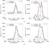 |
Fig. 5 Fitted spectra for Flare 1 using the brightest pixels for Footpoints 1 and 2 – plots a) and b) respectively. For both spectral profiles the total fit and data is shown in black solid and dashed lines respectively. The calibrated 1σ errors on each data point are also plotted including the reduced χ2 value for the fit. The oxygen lines forming the diagnostic ratio are plotted in red in both columns, with the various blends described by the legend. |
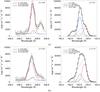 |
Fig. 6 As for Fig. 5 but showing spectra from Flare 2, Footpoints 1 and 2 – plots a) and b) respectively. |
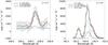 |
Fig. 7 As described in Fig. 5 but with a sample spectra taken from a non-flaring region 55′′ to the north of the Flare 1 footpoints – note the dominant Fe xi contribution in the green dashed line. |
3.2. Densities
The footpoint densities were found by comparing the measured ratio to the diagnostic curve in Fig. 1, and our results are given in Table 2. Taking the absolute error from the fit parameters for width and peak intensity, the error in total intensity of the 192 Å and 248 Å lines can be calculated, and thus the error on the ratio. An estimate of the density error is made by taking these limits on the ratio and finding an upper and lower limit to the density on the diagnostic curve.
O v footpoint densities derived from the I192/I248 ratio.
In all of the footpoints we find that the “pixel” derived density is between log ne (cm-3) = 11.3−11.9, in line with the measurements from Skylab and UVSP where the density varied between log ne = 11.5−12.5 (Cheng et al. 1982; Keenan et al. 1991). Flare 2 FP2 suggests that the density may be slightly over log ne = 12.0 given the uncertainties and our conservative fitting.
Checking the results for the box-averaged method reveals similar densities with a tendency to lower values in all pixels. In Sect. 2.1 we noted that Flare 1 FP1 has an unexplained shift in the position of the footpoint in 248 Å relative to 192 Å and was omitted from the pixel-method results. Using the box method it shows a density of log ne = 11.34. The EIS pixel size is most likely large compared to the EUV footpoint area and this is some evidence to show that higher densities may be revealed when observing on smaller scales; indeed recent results from the Interface Region Imaging Spectrograph (IRIS; De Pontieu et al. 2014) are beginning to show that the footpoint scales are below the EIS spatial resolution (for example Young et al. 2015).
4. Understanding the assumptions
The high densities in Flare 2 should be examined carefully considering the effect of relaxing the assumptions of optically thin plasma in ionisation equilibrium, under which the CHIANTI diagnostic curves are calculated. In this section we calculate the optical depth for both diagnostic lines in two semi-empirical atmospheric models: the VAL-E bright network model (Vernazza et al. 1981), representing the case that the atmosphere is heated without having time to respond hydrodynamically, and the F1 model (Machado et al. 1980) representing the structure of an atmosphere that has already adapted to flare energy input. Additionally, we investigate the diagnostic curves for non-equilibrium line formation temperatures.
4.1. Optical depth
The optical depth at line centre for both O v lines is calculated using the expression in Mihalas (1978; used to the same effect in Dzifčáková & Kulinová 2011 for Si iii transitions). Assuming a thermal Gaussian absorption profile, where ΔνD = (ν0/c)(2kT/M)1/2, the optical depth at line centre is given by 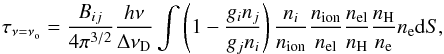 (1)where Bij is the Einstein absorption coefficient from the lower level i to upper level j. Bij can be expressed in terms of the radiative decay coefficient,
  (2)where gi and gj are the statistical weights for levels i and j and Aji is the Einstein coefficient for spontaneous de-excitation. Crucially, the terms inside the integral depend on position in the atmosphere; the relative population of level i, ni/nion is sensitive to density, the ion abundance nion/nel is strongly dependent on temperature, and nH/ne varies with depth. These parameters are taken from the CHIANTI database and we assume constant photospheric abundances, nel/nH, given by Grevesse & Sauval (1998).
The optical depth at line centre is found for both lines by integrating from a chosen depth through the atmosphere above it, and in Figs. 8a and b we show how it varies with temperature for both the VAL-E and the F1 atmospheres. The optical depth quickly plateaus where the ion abundance peaks, as the absorbing ion is not yet formed at lower temperatures. The 192 Å line always remains below τ = 1 whereas 248 Å remains completely optically thin with τ< 10-8. The large difference in optical depths between the lines is mostly due to the difference in population of their lower levels. The optically thin assumption in this case is valid for both lines, and the diagnostic ratio should not be altered.
We should however note that Eq. (1) considers only the balance between the absorption of photons and spontaneous and stimulated emission, where the absorption profile is equal to the emission profile. A more complete description would include the redistribution of the level population within the ion due to the difference in opacity between the lines, or if the absorption and emission profiles are not equal. Certainly the analytical work by Kerr et al. (2004) and observations by Keenan et al. (2014) have shown that viewing-angle dependent enhancements, or suppressions, over the expected optically thin ratio are possible if one line has a significant optical depth. Without performing a similar detailed calculation it is not clear which way our diagnostic ratio would be altered, if at all.
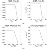 |
Fig. 8 Optical depth at line centre for the oxygen lines in both the VAL-E bright network (top row) and F1 flare atmospheres (bottom row) as function of temperature. |
4.2. Ionisation equilibrium
During the flare onset the footpoint plasma temperature may rise faster than local ionisation processes can occur. For example the peak formation temperature of O v will be shifted to higher temperatures, although the modelling by Bradshaw (2009) predicts that the effect is small at high densities. Nevertheless, we show the effect on the diagnostic curve in Fig. 9 where the diagnostic ratio has been calculated at various plasma temperatures; from the line formation temperature in equilibrium, to the peak of the temperature distribution of a hot footpoint (Graham et al. 2013). For ratios close to those measured, i.e. ~2.3 in Flare 2 FP2, the diagnostic density will range from log ne = 11.85−12.25 depending on the degree of non-equilibrium ionisation, therefore for a sufficiently rapid temperature change the measured densities may be a lower limit.
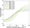 |
Fig. 9 O vλ192/248 diagnostic curves calculated for varying plasma temperature. |
5. Flare heating of dense plasma
After detailed analysis of high resolution Hinode/EIS spectra we can confirm the presence of footpoint densities up to log ne ~ 11.9 at a temperature of 2.5 × 10⁵ K.
Here we investigate the energy input required to produce the observed temperature and density in the same two semi-empirical atmospheric models as Sect. 4; the VAL-E bright network model and the F1 flare model. Heating of the O v emitting region by both accelerated particles, and thermal conduction are considered in turn. The heating rates by accelerated particles are also calculated for each model using a modified, completely ionised density structure, which is a reasonable assumption as the appearance of highly ionised states of oxygen, iron, and calcium is clear evidence that the emitting region is ionised by rapid heating and collisions (Allred et al. 2005).
The two model atmospheres are plotted in Figs. 10a and b. In the VAL-E model, the electron density only reaches log ne = 11.5 below 500 km, well into the temperature minimum region. The structure of the F1 model is similar to VAL-E, except that the transition region has been “pushed” down to around 1400 km (note the different x-axis scales) and the density enhanced up to log ne = 12 at higher altitudes. The completely static model may be a strong assumption however, as pressure-driven density enhancements may occur during rapid heating. In future we plan to extend this work to include atmospheric structures calculated from radiative hydrodynamic codes, e.g. Fisher et al. (1985) and Allred et al. (2005).
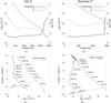 |
Fig. 10 Semi-empirical atmospheric models for a bright network element (Vernazza et al. 1981, VAL-E) and a flare (Machado et al. 1980), panels a) and b), are plotted using tabulated results from their respective papers. In the lower panels, c) and d), the heating rate per particle, deposited by streaming electrons in a collisional thick-target regime, is shown as a function of density within the respective model atmosphere, and for both the model ionisation fraction (diamonds) and a modified atmosphere with constant ionisation fraction x = 1 (crosses). The radiative loss rate per particle, neΛ(T), at the O v formation temperature is also displayed. |
5.1. Electron-beam heating of the O v emitting region
The impulsive phase of Flare 2 (14:13 UT) was captured by RHESSI, and imaging and spectral analysis was presented in Milligan & Dennis (2009). A thermal plus non-thermal power law fit to the integrated spectra gave a low energy cut off of EC = 13 ± 2 keV with a spectral index of δ = 7.6 ± 0.7. The estimated area of 3 × 1017 cm returned a flux in the non-thermal tail of FP = 5 × 10¹⁰ ergs cm-2 s-1. In the following we use these parameters to calculate the heating rate per particle deposited by an injected distribution of non-thermal electrons, above the cut-off energy EC, as a function of height within both model atmospheres. Flare 2 was the only event from this active region with consistent RHESSI coverage, although similar HXR parameters have been obtained in other medium sized events (Graham et al. 2011). We therefore expect this to be fairly typical among other small confined flares and representative also of Flare 1.
We calculate the heating rate per hydrogen nucleus as a function of column depth, Q(N), for a collimated beam (μo = 1) as given by Emslie (1978), with corrections for β (Emslie 1981). The rate is expressed as ![Mathematical equation: \begin{equation} Q(N) = {1 \over 2} {K \gamma (\delta-2) \over \mu_{\rm o}} B\left( {\delta \over 2}, {2\over (4 + \beta)} \right) {F_{\rm P} \over {E_\mathrm{C}^2}} \left[{N} \over N_{\rm c} \right]^{-\delta/2}~{\rm ergs~s^{-1}}, \end{equation}](/articles/aa/full_html/2015/12/aa25348-14/aa25348-14-eq92.png) (3)where K = 2πe4,
(3)where K = 2πe4,  and the Coulomb logarithm for an ionised target, Λ, and effective Coulomb logarithms for neutral targets, Λ′ and Λ′′, are given in Hawley & Fisher (1994). The ionisation fraction, x, can be either assumed to be constant or estimated from the ratio of model electron density to hydrogen density.
The column depth, N, represents the quantity of material traversed by the electron beam. From the atmospheric profiles in Figs. 10a and b we obtain the column depth as a function of height by integrating  at each position in the atmosphere, where nH is the hydrogen density and S is the height in the model atmosphere. The heating rate, Q, is then easily evaluated at each height. To aid the interpretation of the diagnostic results, Q is plotted in Figs. 10c and d against the model electron density, for both model derived and fully ionised density structures (diamonds and crosses respectively). As Q is not expressed as a function of electron density, only of column depth, the reader should be aware that the heating rate can have two values at a single density. The model heights at some intermediate points are plotted for clarity.
Predictably, we find that the heating rate falls off rapidly with increasing depth, especially in the final few 100 km towards the photosphere. The optically thin radiative loss rate per particle, neΛ(T), was taken from CHIANTI for the O v formation temperature above. The point where this line intersects the heating rate indicates where the atmosphere, if heated to O v temperatures, will radiate energy away as quickly as it is deposited, by optically-thin radiative losses. In deeper layers the energy deposition cannot deliver enough energy to raise the ambient temperature.
For the model ionisation structure, given by ne/nH, the critical density for zero net heating in the VAL-E model is approximately log ne = 12.2, and in the F1 atmosphere log ne = 12.4. The measurements for Flare 1 and 2 are below these values, putting them in a region which is possible to heat. The maximum density observed, log ne = 11.89, implies that heating by electrons in both atmospheres must reach a height of ~450 km to produce the required O v emission. However, if the plasma is far from ionisation equilibrium (see Fig. 9) the measured densities imply that the emitting region may be much closer to the heating limit.
If we assume that both atmospheres are completely ionised, i.e ne = nH, then the heating rate intersects the radiative loss rate at a density ~3 orders of magnitude higher. The O v emitting region therefore occurs much higher, at approximately 1600 km for VAL-E and 1450 km for F1, where the heating rate far exceeds the radiative losses. Without a further diagnostic to directly probe the ionisation state throughout the atmosphere we can only deduce that the location of heating lies somewhere between the two cases shown, i.e 450–1600 km.
5.2. Conductive heating of the O v emitting region
In addition to any source of direct heating there may be a significant or dominant conductive energy transport into the deeper layers of the atmosphere. The emission measure distributions obtained in Graham et al. (2013) were consistent with a flaring chromosphere that was in conductive and radiative balance, where a directly heated layer at 10 MK supplied a conductive flux to the chromosphere below, balanced by radiative losses.
In a steady-state atmosphere with no dynamic flows the energy balance equation is,  (6)where FC is the conductive flux, ER is the radiative loss rate, and EH the heating rate from additional sources. If we assume that no direct heating reaches the region where conductive energy input is balanced by radiative losses, then
  (7)for a radiative loss rate Λ(T) at the temperature of O v formation (log T = 5.4). The conductive flux in 1D is expressed as
  (8)where κo = 9.2 × 10⁻⁷ for classical Spitzer conductivity. The temperature gradient or length scales are not known in the chromosphere, and the conductive flux can only be estimated. However, by making some simple assumptions we can estimate the scale of the emitting region required to balance a purely conductive heating term. In 1D the conductive term in Eq. (7) then becomes
  (9)If the top of the chromosphere is impulsively heated to Tmax = 10 MK then we can replace dT/ dS with (Tmax − T) /L, where T is the temperature of the plasma that is emitting oxygen lines, and L is the chromospheric scale length required to balance conductive energy inputs with radiative losses. By assuming a uniform temperature gradient, i.e. d2T/ dS2 = 0, the conductive flux for a scale length in units of km becomes
  (10)By rearranging Eq. (7), and inserting the result above, the chromospheric length scale L is
  (11)Our requirement is to supply enough conductive flux to the chromosphere below a 10 MK layer to allow plasma at T = 105.4 K to radiate. The density of the chromosphere will vary with depth, but if we assume that the average density of the whole region is between 1011−1012 cm-3 then the conductive input will be balanced by the radiative losses for a chromosphere of thickness 70–700 km. Inspecting the atmospheres in Figs. 10a and b shows that these thicknesses are reasonable within the picture of a compressed, lower altitude transition region. However, the semi-empirical models shown do not include a sufficiently high temperature component at ~10 MK, as found by several more recent studies (Mrozek & Tomczak 2004; Brosius 2012; Graham et al. 2013; Fletcher et al. 2013).
6. Conclusions
The location, or depth in a 1D interpretation, of energy deposition within the flaring chromosphere remains an important constraint on the global plasma behaviour of the flaring chromosphere. We have presented in this paper new confirmation of 250 000 K footpoint plasma with electron densities of log ne (cm-3) = 11.3−11.9 in two flares. The assumption of optically-thin plasma was tested and found to be acceptable for these lines using two model atmospheres. The effect of non-equilibrium ionisation on the diagnostic was taken into consideration and found to alter the measured density, potentially raising the maximum density observed to log ne (cm-3) ~ 12.2, although further modelling is required to determine how significant the effect is during the impulsive phase.
With our measurement of the electron density (and knowledge of the temperature) of the O v emitting region we have been able to estimate its properties under different assumptions about the energy input. Assuming an atmosphere structured according to VAL-E or F1, the emitting region is found ~450 km above the photosphere. The collisional beam heating rate is found to exceed the radiative losses here, although if the density was slightly higher, log ne (cm-3) > 12.4, then radiative losses would balance the heating input.
If the calculation is repeated for the VAL-E and F1 mass density structure but assuming complete ionisation then the O v emitting region is found around 1450–1600 km above the photosphere, where the heating input rate easily exceeds the radiative losses. As the ionisation fraction is unknown we determine the heating location to be between 450–1600 km.
Energy transport from a directly heated slab via a conduction flux was also considered and can provide the necessary O v emission given a chromosphere of thickness between 70–700 km. The thickness is reasonable considering the emission heights that we have estimated. A combination of both transport methods will be considered in future, including conductive losses to the lower atmosphere.
The ionisation state of the flaring chromosphere clearly plays an important role in determining the energy balance in flare footpoints and on diagnostics of this kind. By coupling further temperature and density diagnostics with radiative-hydrodynamic models, and including new observations of ionisation/recombination signatures (Heinzel & Kleint 2014), then the location of the emitting region may be better constrained.
Finally, this work shows that diagnostics of high density plasmas are of great value, as was seen in the past by the Skylab and UVSP spectrographs, yet few studies of this kind have been made in recent years. Whilst it is possible with EIS to make this particular diagnostic, the long wavelength detector is degrading (Del Zanna 2013) and the 248 Å line is becoming difficult to observe without a specifically targeted EIS study (longer exposures may be necessary which are not best suited to flare observations). The Extreme-Ultraviolet Variability Experiment (Woods et al. 2012) measures the strong O v 629.73 Å to 760.30 Å ratio among others, but footpoint identification is difficult with no spatial resolution. Data from IRIS is extremely promising though, as the O iv 1404.78 Å to 1399.77 Å ratio (Dudík et al. 2014) should provide a useful diagnostic at transition region temperatures and with improved spatial and temporal resolution.
Acknowledgments
D.R.G. acknowledges support from an STFC-STEP award. L.F. and N.L. acknowledge support from STFC-funded rolling grant ST/F002637/1. The research leading to these results has received funding from the European Community’s Seventh Framework Programme (FP7/2007-2013) under grant agreement No. 606862 (F-CHROMA). CHIANTI is a collaborative project involving the NRL (USA), the Universities of Florence (Italy) and Cambridge (UK), and George Mason University (USA). We are grateful for the open data policies of RHESSI and Hinode and the efforts of the instrument and software teams. Hinode is a Japanese mission developed and launched by ISAS/JAXA, with NAOJ as domestic partner and NASA and STFC (UK) as international partners. It is operated by these agencies in co-operation with ESA and NSC (Norway). We would also like to thank Peter Young and Jaroslav Dudik for their discussion and helpful comments.
References
- Allred, J. C., Hawley, S. L., Abbett, W. P., & Carlsson, M. 2005, ApJ, 630, 573 [NASA ADS] [CrossRef] [Google Scholar]
- Antonucci, E., & Dennis, B. R. 1983, Sol. Phys., 86, 67 [NASA ADS] [CrossRef] [Google Scholar]
- Bartoe, J.-D. F., Brueckner, G. E., Purcell, J. D., & Tousey, R. 1977, Appl. Opt., 16, 879 [NASA ADS] [CrossRef] [Google Scholar]
- Bradshaw, S. J. 2009, A&A, 502, 409 [NASA ADS] [CrossRef] [EDP Sciences] [Google Scholar]
- Brosius, J. W. 2012, ApJ, 754, 54 [NASA ADS] [CrossRef] [Google Scholar]
- Brown, J. C., Turkmani, R., Kontar, E. P., MacKinnon, A. L., & Vlahos, L. 2009, A&A, 508, 993 [NASA ADS] [CrossRef] [EDP Sciences] [Google Scholar]
- Cheng, C.-C., Bruner, E. C., Tandberg-Hanssen, E., et al. 1982, ApJ, 253, 353 [NASA ADS] [CrossRef] [Google Scholar]
- Czaykowska, A., De Pontieu, B., Alexander, D., & Rank, G. 1999, ApJ, 521, L75 [NASA ADS] [CrossRef] [Google Scholar]
- De Pontieu, B., Title, A. M., Lemen, J. R., et al. 2014, Sol. Phys., 289, 2733 [NASA ADS] [CrossRef] [Google Scholar]
- Del Zanna, G. 2013, A&A, 555, A47 [NASA ADS] [CrossRef] [EDP Sciences] [Google Scholar]
- Del Zanna, G., Mitra-Kraev, U., Bradshaw, S. J., Mason, H. E., & Asai, A. 2011, A&A, 526, A1 [NASA ADS] [CrossRef] [EDP Sciences] [Google Scholar]
- Dere, K. P., Landi, E., Mason, H. E., Monsignori Fossi, B. C., & Young, P. R. 1997, A&AS, 125, 149 [NASA ADS] [CrossRef] [EDP Sciences] [Google Scholar]
- Doschek, G. A., Feldman, U., & Rosenberg, F. D. 1977, ApJ, 215, 329 [NASA ADS] [CrossRef] [Google Scholar]
- Dudík, J., Del Zanna, G., Dzifčáková, E., Mason, H. E., & Golub, L. 2014, ApJ, 780, L12 [NASA ADS] [CrossRef] [Google Scholar]
- Dzifčáková, E., & Kulinová, A. 2011, A&A, 531, A122 [NASA ADS] [CrossRef] [EDP Sciences] [Google Scholar]
- Emslie, A. G. 1978, ApJ, 224, 241 [NASA ADS] [CrossRef] [Google Scholar]
- Emslie, A. G. 1981, ApJ, 245, 711 [NASA ADS] [CrossRef] [Google Scholar]
- Feldman, U., Dorschek, G. A., & Rosenberg, F. D. 1977, ApJ, 215, 652 [NASA ADS] [CrossRef] [Google Scholar]
- Fisher, G. H., Canfield, R. C., & McClymont, A. N. 1985, ApJ, 289, 425 [NASA ADS] [CrossRef] [Google Scholar]
- Fletcher, L., & Hudson, H. S. 2008, ApJ, 675, 1645 [NASA ADS] [CrossRef] [Google Scholar]
- Fletcher, L., Hannah, I. G., Hudson, H. S., & Innes, D. E. 2013, ApJ, 771, 104 [NASA ADS] [CrossRef] [Google Scholar]
- Graham, D. R., Fletcher, L., & Hannah, I. G. 2011, A&A, 532, A27 [NASA ADS] [CrossRef] [EDP Sciences] [Google Scholar]
- Graham, D. R., Hannah, I. G., Fletcher, L., & Milligan, R. O. 2013, ApJ, 767, 83 [NASA ADS] [CrossRef] [Google Scholar]
- Grevesse, N., & Sauval, A. J. 1998, Space Sci. Rev., 85, 161 [NASA ADS] [CrossRef] [Google Scholar]
- Hawley, S. L., & Fisher, G. H. 1994, ApJ, 426, 387 [NASA ADS] [CrossRef] [Google Scholar]
- Heinzel, P., & Kleint, L. 2014, ApJ, 794, L23 [NASA ADS] [CrossRef] [Google Scholar]
- Keenan, F. P., Dufton, P. L., Harra, L. K., et al. 1991, ApJ, 382, 349 [NASA ADS] [CrossRef] [Google Scholar]
- Keenan, F. P., Doyle, J. G., Madjarska, M. S., et al. 2014, ApJ, 784, L39 [NASA ADS] [CrossRef] [Google Scholar]
- Kerr, F. M., Rose, S. J., Wark, J. S., & Keenan, F. P. 2004, ApJ, 613, L181 [NASA ADS] [CrossRef] [Google Scholar]
- Ko, Y.-K., Doschek, G. A., Warren, H. P., & Young, P. R. 2009, ApJ, 697, 1956 [NASA ADS] [CrossRef] [Google Scholar]
- Kulinová, A., Kašparová, J., Dzifčáková, E., et al. 2011, A&A, 533, A81 [NASA ADS] [CrossRef] [EDP Sciences] [Google Scholar]
- Landi, E., Young, P. R., Dere, K. P., Del Zanna, G., & Mason, H. E. 2013, ApJ, 763, 86 [NASA ADS] [CrossRef] [Google Scholar]
- Lin, R. P., Dennis, B. R., Hurford, G. J., et al. 2002, Sol. Phys., 210, 3 [Google Scholar]
- Liu, W., Petrosian, V., & Mariska, J. T. 2009, ApJ, 702, 1553 [NASA ADS] [CrossRef] [Google Scholar]
- Machado, M. E., Avrett, E. H., Vernazza, J. E., & Noyes, R. W. 1980, ApJ, 242, 336 [NASA ADS] [CrossRef] [Google Scholar]
- Mariska, J. T., & Poland, A. I. 1985, Sol. Phys., 96, 317 [NASA ADS] [CrossRef] [Google Scholar]
- Mihalas, D. 1978, Stellar atmospheres, 2nd edn. [Google Scholar]
- Milligan, R. O. 2011, ApJ, 740, 70 [NASA ADS] [CrossRef] [Google Scholar]
- Milligan, R. O., & Dennis, B. R. 2009, ApJ, 699, 968 [NASA ADS] [CrossRef] [Google Scholar]
- Mrozek, T., & Tomczak, M. 2004, A&A, 415, 377 [NASA ADS] [CrossRef] [EDP Sciences] [Google Scholar]
- Nagai, F., & Emslie, A. G. 1984, ApJ, 279, 896 [NASA ADS] [CrossRef] [Google Scholar]
- Poland, A. I., Orwig, L. E., Mariska, J. T., Auer, L. H., & Nakatsuka, R. 1984, ApJ, 280, 457 [NASA ADS] [CrossRef] [Google Scholar]
- Russell, A. J. B., & Fletcher, L. 2013, ApJ, 765, 81 [NASA ADS] [CrossRef] [Google Scholar]
- Vernazza, J. E., Avrett, E. H., & Loeser, R. 1981, ApJS, 45, 635 [NASA ADS] [CrossRef] [Google Scholar]
- Warren, H. P., Ugarte-Urra, I., & Landi, E. 2014, ApJS, 213, 11 [NASA ADS] [CrossRef] [Google Scholar]
- Watanabe, T., Hara, H., Sterling, A. C., & Harra, L. K. 2010, ApJ, 719, 213 [NASA ADS] [CrossRef] [Google Scholar]
- Widing, K. G., Doyle, J. G., Dufton, P. L., & Kingston, E. A. 1982, ApJ, 257, 913 [NASA ADS] [CrossRef] [Google Scholar]
- Woodgate, B. E., Brandt, J. C., Kalet, M. W., et al. 1980, Sol. Phys., 65, 73 [NASA ADS] [CrossRef] [Google Scholar]
- Woods, T. N., Eparvier, F. G., Hock, R., et al. 2012, Sol. Phys., 275, 115 [Google Scholar]
- Young, P. R., Del Zanna, G., Mason, H. E., et al. 2007, PASJ, 59, 727 [Google Scholar]
- Young, P. R., Watanabe, T., Hara, H., & Mariska, J. T. 2009, A&A, 495, 587 [NASA ADS] [CrossRef] [EDP Sciences] [Google Scholar]
- Young, P. R., Tian, H., & Jaeggli, S. 2015, ApJ, 799, 218 [NASA ADS] [CrossRef] [Google Scholar]
All Tables
All Figures
|
Fig. 1 Diagnostic ratio for O v 192.904 Å/248.460 Å. |
| In the text | |
|
Fig. 2 Fitted intensities in several different temperature lines for the 01:35:28 UT raster (Flare 1) after correcting for the EIS detector offset. White dotted lines show the position of the footpoints in each image relative to the O v 192 Å line. The x-offset is highlighted by the black strip on the left of the Fe xiv 274 Å image. |
| In the text | |
|
Fig. 3 Density sensitivity of the blended O v lines with respect to the 192.904 Å transition. |
| In the text | |
|
Fig. 4 Intensity maps for both 192.904 Å and 248.460 Å lines corresponding to the impulsive phase for both flares. Two footpoints regions (1 and 2) are bounded in each flare by a white box (pixels under the line are included in the selection). The brightest pixel within each footpoint region is also identified by a black cross. |
| In the text | |
|
Fig. 5 Fitted spectra for Flare 1 using the brightest pixels for Footpoints 1 and 2 – plots a) and b) respectively. For both spectral profiles the total fit and data is shown in black solid and dashed lines respectively. The calibrated 1σ errors on each data point are also plotted including the reduced χ2 value for the fit. The oxygen lines forming the diagnostic ratio are plotted in red in both columns, with the various blends described by the legend. |
| In the text | |
|
Fig. 6 As for Fig. 5 but showing spectra from Flare 2, Footpoints 1 and 2 – plots a) and b) respectively. |
| In the text | |
|
Fig. 7 As described in Fig. 5 but with a sample spectra taken from a non-flaring region 55′′ to the north of the Flare 1 footpoints – note the dominant Fe xi contribution in the green dashed line. |
| In the text | |
|
Fig. 8 Optical depth at line centre for the oxygen lines in both the VAL-E bright network (top row) and F1 flare atmospheres (bottom row) as function of temperature. |
| In the text | |
|
Fig. 9 O vλ192/248 diagnostic curves calculated for varying plasma temperature. |
| In the text | |
|
Fig. 10 Semi-empirical atmospheric models for a bright network element (Vernazza et al. 1981, VAL-E) and a flare (Machado et al. 1980), panels a) and b), are plotted using tabulated results from their respective papers. In the lower panels, c) and d), the heating rate per particle, deposited by streaming electrons in a collisional thick-target regime, is shown as a function of density within the respective model atmosphere, and for both the model ionisation fraction (diamonds) and a modified atmosphere with constant ionisation fraction x = 1 (crosses). The radiative loss rate per particle, neΛ(T), at the O v formation temperature is also displayed. |
| In the text | |
Current usage metrics show cumulative count of Article Views (full-text article views including HTML views, PDF and ePub downloads, according to the available data) and Abstracts Views on Vision4Press platform.
Data correspond to usage on the plateform after 2015. The current usage metrics is available 48-96 hours after online publication and is updated daily on week days.
Initial download of the metrics may take a while.