| Issue |
A&A
Volume 583, November 2015
|
|
|---|---|---|
| Article Number | A69 | |
| Number of page(s) | 9 | |
| Section | Galactic structure, stellar clusters and populations | |
| DOI | https://doi.org/10.1051/0004-6361/201526592 | |
| Published online | 29 October 2015 | |
NGC 6139: a normal massive globular cluster, or a first-generation dominated cluster? Clues from the light elements ⋆,⋆⋆,⋆⋆⋆
1
INAF–Osservatorio Astronomico di Bologna, via Ranzani 1,
40127
Bologna,
Italy
e-mail:
This email address is being protected from spambots. You need JavaScript enabled to view it.
2
Dipartimento di Fisica e Astronomia, Università di
Bologna, viale Berti Pichat
6, 40127
Bologna,
Italy
3
INAF–Osservatorio Astronomico di Padova, Vicolo dell’Osservatorio
5, 35122
Padova,
Italy
4
Monash Centre for Astrophysics, School of Physics and Astronomy,
Monash University, Melbourne, VIC
3800,
Australia
5
Department of Physics and Astronomy, Macquarie
University, Sydney,
NSW
2109,
Australia
6
Department of Astronomy and McDonald Observatory, The University
of Texas, Austin,
TX
78712,
USA
Received: 25 May 2015
Accepted: 30 July 2015
Abstract
Information on globular clusters (GC) formation mechanisms can be gathered by studying the chemical signature of the multiple populations that compose these stellar systems. In particular, we investigate the anti-correlations among O, Na, Al, and Mg to explore the influence of cluster mass and environment on GCs in the Milky Way and in extragalactic systems. We present here the results obtained on NGC 6139, which, on the basis of its horizontal branch morphology, has been proposed to be dominated by first-generation stars. In our extensive study based on high-resolution spectroscopy, the first for this cluster, we found a metallicity of [Fe/H] = −1.579 ± 0.015 ± 0.058 (rms = 0.040 dex, 45 bona fide member stars) on the UVES scale defined by our group. The stars in NGC 6139 show a chemical pattern normal for GCs, with a rather extended Na-O (and Mg-Al) anti correlation. NGC 6139 behaves as expected from its mass and contains a large portion (about two thirds) of second-generation stars.
Key words: stars: abundances / stars: atmospheres / stars: Population II / Galaxy: general / globular clusters: general / globular clusters: individual: NGC 6139
Based on observations collected at ESO telescopes under programme 093.B-0583 and on data obtained from the ESO Science Archive Facility under request number 94403.
Appendix A is available in electronic form at http://www.aanda.org
The final photometric catalogue is only available at the CDS via anonymous ftp to cdsarc.u-strasbg.fr (130.79.128.5) or via http://cdsarc.u-strasbg.fr/viz-bin/qcat?J/A+A/583/A69
© ESO, 2015
1. Introduction
Once considered as a good example of simple stellar populations, Galactic globular clusters (GCs) are currently thought to have formed in a complex chain of events, which left a fossil record in their chemical composition (see e.g., the review by Gratton et al. 2012). Photometrically, GCs often exhibit spread, split, and even multiple sequences that can be explained by different chemical composition among cluster stars, in particular of light elements such as He, C, N, and O (e.g., Carretta et al. 2011b; Sbordone et al. 2011; Milone et al. 2012a; Piotto et al. 2015). Our FLAMES survey of more than 20 Milky Way (MW) GCs (see Carretta et al. 2009a, 2014b, and references therein) combined with literature data, demonstrated that most, perhaps all, GCs host multiple stellar populations (see Carretta et al. 2010a). Variations of Na and O (and sometimes of Mg and Al) abundances trace these different sub-populations.
Our large and homogeneous database allowed us a quantitative study of the Na-O anti-correlation. In all the analysed GCs we found about one third of stars to be of primordial composition, similar to that of field stars of similar metallicity (low Na, high O), which means that they belong to the first generation (FG). The other two thirds have a modified composition (increased Na, depleted O) and belong to the second generation (SG) of stars, which is polluted by the FG (see, e.g., Carretta et al. 2009a,b). It is still debated which were the more massive stars of the FG that produced the gas of modified composition, see for instance Decressin et al. (2007), Ventura et al. (2001), or Bastian et al. (2013) for an alternative view.
We also found that the extension of the Na-O anti-correlation tends to be larger for higher mass GCs and that, apparently, there is an observed minimum cluster mass for the appearance of the Na-O anti-correlation (Carretta et al. 2010a). It is important to understand whether this limit is due to the small statistics (fewer low-mass clusters have been studied, and only a few stars were observed in each). This in an important constraint for cluster formation mechanisms because it indicates the mass at which we expect that a cluster is able to retain part of the ejecta of the FG, hence to show the Na-O signature (the masses of the original clusters are expected to be much higher than the present ones, since the SG has to be formed by the ejecta of the FG).
Variations in Na, O, and He are connected with each other, but do not tell us exactly the same story. The effects of increased He are visible in colour-magnitude diagrams (CMD) in the main-sequence (MS) phase (e.g., Piotto et al. 2007) or, more evidently, in the horizontal branch phase (HB, e.g., D’Antona et al. 2005; Gratton et al. 2010; Milone et al. 2014). Based on the possibility of reproducing their HBs with a single He value, Caloi & D’Antona (2011) proposed that some GCs are composed of a single generation (FG-only) or predominantly by a single generation (mainly-FG). It would be important to measure their Na, O, and Al abundances to clarify the issue. Al, which is only produced at higher temperatures than Na (e.g., Prantzos et al. 2007, for an application to the GC peculiar chemistry), that is, by more massive stars, should follow the He enrichment better than Na (and O). We can then expect to find Na and O variations without significant He enhancement; this would produce short HBs (and no variations in Al)1. In summary, we would be in presence of FG and SG stars even without significant He variations; this is important to understand the cluster formation and early intracluster gas pollution.
After studying the high-mass clusters, we began a systematic study of low-mass GCs, FG-only and mainly-FG GCs, and high-mass and old open clusters (OCs). Our goal is to empirically find the mass limit for the appearance of the Na-O anti-correlation and to ascertain whether there are differences between high-mass and low-mass cluster properties, for instance in the relative fraction of FG and SG stars.
We also included GCs belonging to the Sagittarius dwarf spheroidal galaxy (Sgr dSph) to study whether there are differences in GCs formed in different environments (the MW and dwarf galaxies). GCs born in a dSph are expected to have experienced a milder tidal field, thus possibly retaining a larger portion of their original mass. Only a few old GCs in Fornax and LMC have their abundances derived using high-resolution spectroscopy. These GCs also seem to host two populations (Letarte et al. 2006; Johnson et al. 2006; Mucciarelli et al. 2009), but the fractions of FG and SG stars in Fornax and LMC GCs of similar mass seem different. Is this again a problem of low statistics, or is the galactic environment (a dwarf spheroidal vs. a dwarf irregular) influencing the GC formation mechanism? This is outside the main theme of this paper, and we refer to Larsen et al. (2012), D’Antona et al. (2013) for a more detailed discussion.
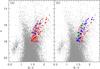 |
Fig. 1 a) CMD of NGC 6139, with its quite short blue HB. In grey we plot all stars, in red all targets observed with FLAMES. The seven UVES stars are indicated by blue open squares; the stars with RV from Saviane et al. (2012) are represented by blue crosses. b) The non-member stars (and the star on the HB) are indicated by red open squares, the stars that are candidate members on the basis of their RV by filled blue squares. The member stars define a reasonably tight RGB, and we indicate with green circles the probable AGB stars (see Sect. 3.1) |
We have already gathered high-resolution spectra of a low-mass GC (NGC 6535, which will be analysed in a forthcoming paper), two high-mass OCs (Berkeley 39, NGC 6791, see Bragaglia et al. 2012, 2014), a proposed FG-only GC (NGC 6139, this paper), and Terzan 8 (Carretta et al. 2014a), which belongs to the Sgr dSph. In Terzan 8 we see some indication of a SG, at variance with other low-mass Sgr GCs (Ter 7, Pal 12, Tautvaišienė et al. 2004; Sbordone et al. 2007; Cohen 2004) or to Rup 106 (Villanova et al. 2013). However, in Terzan 8 the SG seems to be a minority component, in contrast to what occurs for high-mass GCs. The Na-O anti-correlation has never been observed in OCs (de Silva et al. 2009; MacLean et al. 2014), and we confirmed this using large samples of stars both for Berkeley 39 (Bragaglia et al. 2012) using FLAMES spectra and NGC 6791 (Bragaglia et al. 2014) using Hydra at WIYN and HIRES at Keck spectra. In particular, for NGC 6791, where Geisler et al. (2012) claimed to have found some variations in Na, O, we did not detect any evidence of this trend. Our findings are corroborated by independent works, see Cunha et al. (2015), Boesgaard et al. (2015).
We concentrate here on the possibly FG-only cluster NGC 6139. In Sect. 2 we present literature information on the cluster, and in Sect. 3 we describe the photometric data and the spectroscopic observations and derive the atmospheric parameters. The abundance analysis is presented in Sect. 4, and we discuss the light-element abundances in Sect. 5.
2. NGC 6139 in literature
NGC 6139 is a massive GC (its absolute visual magnitude, a proxy for mass, is MV = −8.36, Harris 1996) located toward the centre of the MW, at l = 342.37°, b = 6.94°. The cluster has received relatively little attention in the past; in particular, it has never before been studied with high-resolution spectroscopy.
Hazen (1991) found ten variable stars in NGC 6139, five of which are RR Lyrae stars. The four RRab seem to indicate a Oosterhoff type II. A CMD was presented by Samus’ et al. (1996); they employed photographic B and V plates, and their photometry only reached the RGB and HB. They found the cluster to be quite metal-poor (close to [Fe/H] = −2) from the slope of the RGB, and highly reddened. Zinn & Barnes (1998) used VI photometry that barely reached the main-sequence turn-off, noted the high and differential reddening (and corrected for a gradient), and determined [Fe/H] = −1.71 ± 0.20 and a mean reddening of E(V − I) = 1.03 ± 0.04, corresponding to E(B − V) = 0.76 ± 0.03. Similar results were reached by Ortolani et al. (1999) on the basis of VI photometry, and by Davidge (1998), who used near-infrared data and also noted that the differential reddening is not a significant problem, since the RGB sequence becomes very well defined once the field star contamination is statistically removed. Finally, Piotto et al. (2002) presented WFPC2 photometry, as part of their HST snapshot programme (74 MW GCs observed with the F439W and F555W bands), in which the RGB and HB are very well defined, and the main-sequence turn-off is better defined than in previous works. Their data are publicly available, and we used them for the present work (see next section).
The only determination of metallicity based on spectroscopy is reported by Saviane et al. (2012), who used spectra at a resolution of R ~ 2500 in the region of the infrared Ca ii triplet (CaT). NGC 6139 is one of the 20 GCs in the paper. They observed 19 stars, 15 of which were considered members (we used this information to select our targets, see next section). The metallicity they obtained from the CaT lines is [Fe/H] = −1.63, rms = 0.13 (on the metallicity scale defined in Carretta et al. 2009c).
Caloi & D’Antona (2011) included NGC 6139 in their list of candidate FG clusters. They tried to identify clusters whose HB could be reproduced by a single mass (in the framework where the dispersion in mass of HB stars is due -at least in part- to variations in He content, in turn an indication of multiple generations). A first clue is the short HB (similar to the HB of NGC 6397, see Piotto et al. 2002, which, however has both a normal Na-O anti-correlation and a small ΔY; see Carretta et al. 2009a,b; Milone et al. 2012b, respectively). However, given its high mass (log M = 5.58 M⊙, their Table 1), NGC 6139 should have produced a SG, but failed to lose a large part of the FG stars, so it should currently be FG-dominated. Caloi & D’Antona (2011) did not discuss the case for NGC 6139 in detail, but because it was included in the list, combined with the absence of previous high-resolution spectroscopic studies, it was a good target for our on-going programme.
Log of FLAMES observations.
3. Observations and analysis
Of the photometric data discussed in the previous section, only the HST catalogue is publicly available. However, the very small field of view (FoV, about 2′ side) is poorly suited to the FLAMES FoV (25′ diameter). We therefore retrieved from the ESO archive some B and V filter frames acquired (under program 68.D-0265) with the Wide Field Imager (WFI) at the 2.2 m ESO-MPG telescope, which has a FoV of about 30′ side.
They were reduced in the standard way, correcting for bias and flat field using IRAF2. Stars were detected independently in the B and V frames, and the instrumental magnitudes were obtained using the point spread function (PSF) fitting code DAOPHOT-II/ALLSTAR (Stetson 1987, 1993). We employed the 2 Micron All Sky Survey Catalogue (2MASS, Skrutskie et al. 2006) and the CataXcorr code3, developed by P. Montegriffo, to compute the astrometric solution and transform the instrumental pixel coordinates into J2000 celestial coordinates. The astrometric precision is about 0.2 arcsec, perfectly compatible with the requirements of the FLAMES observations. No standard stars were available, so we calibrated our photometry to that of the HST using the stars in common. The final photometric catalogue will be made available through the CDS.
The resulting CMD is shown in Fig. 1. As expected from its Galactic position, the field star contamination is conspicuous, but the cluster RGB and HB are visible, especially in the very central region. The cluster sequences are also affected by differential reddening (DR), as already discussed in the literature. This could be relevant for the spectroscopic analysis, since our atmospheric parameters are derived from photometry. However, as has previously been done for other difficult cases, resorting to optical-IR colours (in particular, V − K), greatly alleviates the problem. For instance, the bulge GC GC 6441 (Gratton et al. 2007) has an rms scatter of 0.05 mag in E(B − V), resulting in random (star-to-star) uncertainties in the effective temperatures of ± 80 K. We roughly evaluated the size of DR for NGC 6139 by defining an RGB ridge line with the help of HST photometry and by projecting the candidate members (see next section) on it along the reddening vector. The average displacement required is 0.03 mag, therefore we expect a possible error of about 50 K.
3.1. FLAMES spectra
NGC 6139 was observed with the multi-object spectrograph FLAMES at VLT (Pasquini et al. 2002). We used the GIRAFFE high-resolution setups HR11, HR13, and HR21 (R = 24 200, 22 500, 16 200, respectively), which contain two Na doublets, the [O i] line at 6300 Å, and the Al doublet at 8772 Å, plus several Mg lines. The observations were performed in service mode; a log is presented in Table 1. The HR11 and HR13 GIRAFFE observations were coupled with the high-resolution (R = 47 000) UVES 580 nm setup (λλ ≃ 4800−6800 Å) and the HR21 observations with the UVES 860 nm setup (λλ ≃ 6600−10 600 Å). We only used the 580nm spectra in this paper for consistency with our previous works and because they have better signal-to-noise ratio.
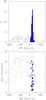 |
Fig. 2 Upper panel: histogram of all measured RVs (open histogram) and of the candidate member stars alone (blue filled histogram). Lower panel: RVs versus distance from the cluster centre. The candidate member stars are indicated by filled blue squares, the UVES targets by large red crosses, and the lines indicate the cluster mean RV and the ± 3σ interval. |
The B,V WFI catalogue was used to select candidate targets for the spectroscopic observations. As for all other GCs in our sample, we only chose stars without close neighbours (≤2.5″). We cross-identified the stars in Saviane et al. (2012) to allocate seven UVES fibres to high-probability cluster members; the eigth fibre was put on an empty spot for sky subtraction. We allocated 103 GIRAFFE fibres to RGB stars, one to an HB star, and 16 to sky positions. All targets are brighter than the RGB bump (V = 17.867 ± 0.019; Nataf et al. 2013). The 111 stars observed are shown in Fig. 1a with different symbols; their coordinates and magnitudes are given in Table A.1 (for candidate members, based on their RV) and Table A.2 (for non-members). All stars observed are within 7 arcmin from the centre, see Fig. 2, lower panel, that is, they are well within the tidal radius (10.5 armin, Harris 1996). Almost all stars observed are beyond the half-mass radius (0.85 arcmin, Harris).
The spectra were reduced using the ESO pipelines for UVES-FIBRE and GIRAFFE data; they take care of bias and flat-field correction, order tracing, extraction, fibre transmission, scattered light, and wavelength calibration. We then used IRAF routines on the 1D wavelength-calibrated individual spectra to subtract the (average) sky, shift to zero RV, and combine all the exposures for each star. The region near the [O i] line required special attention because of the strong sky emission and the many absorptions. Given the low RV of the cluster, the HR13 exposures were scheduled when the Earth motion took the sky emission farther away from the [O i] line of the stars. We also checked that in all these exposures the telluric absorptions did not fall on the line of the stars by visual comparison with a telluric template. The RV was measured using DOOp (Cantat-Gaudin et al. 2014), an automated wrapper for DAOSPEC (Stetson & Pancino 2008); the average, heliocentric value for each star is given in Tables A.1 and A.2.
Sensitivities of abundance ratios to variations in the atmospheric parameters and to errors in the equivalent widths, and errors in abundances for stars of NGC 6139 observed with UVES.
We show in Fig. 2 the histogram of the RVs and a plot of RVs versus distance from cluster centre (taken from the website update in 2010 of Harris 1996); the cluster signature is clear. We are the first to report an estimate of RV based on a large number of stars observed at high resolution; we found ⟨RV⟩ = + 28.88, rms = 7.34 km s-1 (a typical rms for a GC). This value is compatible with the RV = 6.7 ± 6.0 km s-1 in Harris (1996), based on much lower resolution and lower quality data4, and it agrees well with Saviane et al. (2012), who reported a RV = 34 ± 4 km s-1, based on 15 stars (for a direct comparison of RVs for eight stars in common, see Table A.1).
We are left with 50 candidate members based on the RV, that is, falling within ± 3σ of the cluster average. After pruning the sample, the RGB of NGC 6139 is well defined and tight, even in presence of DR (see Fig. 1b). In the following we discuss only these 50 candidates.
Following our well-tested procedure (for a lengthy description, see e.g., Carretta et al. 2009a,b), effective temperatures Teff for our targets were derived using an average relation between apparent magnitudes and first-pass temperatures from V − K colours and the calibrations of Alonso et al. (1999, 2001). This method permits decreasing the star-to-star errors in abundances due to uncertainties in temperatures, since magnitudes are less affected by uncertainties than colours. This is particularly true for NGC 6139, which presents high and variable reddening, for which we used the apparent K magnitudes in our relation with Teff because the effect of the DR on these magnitudes is weaker. The adopted reddening E(B − V) = 0.75 and distance modulus (m − M)V = 17.35 are taken from the catalogue of Harris (1996). Gravities were obtained from apparent magnitudes and distance modulus, assuming the bolometric corrections from Alonso et al. (1999). We adopted a mass of 0.85 M⊙ for all stars and Mbol, ⊙ = 4.75 as the bolometric magnitude for the Sun, as in our previous studies.
Sensitivities of abundance ratios to variations in the atmospheric parameters and to errors in the equivalent widths, and errors in abundances for stars of NGC 6139 observed with GIRAFFE.
We eliminated trends in the relation between abundances from Fe i lines and expected line strength (Magain 1984) to obtain values of the microturbulent velocity vt.
Finally, using the above values, we interpolated within the Kurucz (1993) grid of model atmospheres (with the option for overshooting on) to derive the final abundances, adopting for each star the model with the appropriate atmospheric parameters and whose abundances matched those derived from Fe i lines. Five stars among the candidate members have a metallicity higher by more than 0.5 dex than the average of the others; they are probably field stars and were excluded from the most secure sample of RV plus metallicity members. The atmospheric parameters for all bona fide member stars are given in Table A.3.
Six of the candidate members (two with UVES and four with GIRAFFE spectra) were too metal-poor (by about 0.15 dex); their position in the CMD seemed to indicate that they might be asymptotic giant branch (AGB) and not RGB stars. Following the same procedure as was used for the RGB stars, we derived a separate colour-temperature relation for them, finding temperatures higher by about 110 K. Adopting the new temperatures, we repeated the analysis, finding a metallicity that agreed very well with the cluster average. These second values for Teff and metallicity are given in Table A.3.
4. Abundances
In addition to the abundance of Fe, we present here the abundance of O, Na, Mg, and Al. The last was derived from the Al i doublet at 6696−98 Å for stars observed with UVES and from the doublet at 8772 Å for stars observed with GIRAFFE. The abundance ratios for all elements are given in Table A.4, together with number of lines used and the rms scatter.
The abundances were derived using equivalent widths (EW). We measured the EW of iron and other elements using the code ROSA (Gratton 1988) adopting a relationship between EW and FWHM (for details, see Bragaglia et al. 2001). The atomic data for all the lines in the UVES spectra and in the HR11 and HR13 set-ups and the solar reference values come from Gratton et al. (2003). The Na abundances were corrected for departure form local thermodynamical equilibrium according to Gratton et al. (1999).
The derived Fe abundances do not show any trend with Teff. The average metallicity derived for stars with UVES spectra is [Fe/H] = −1.579 ± 0.015 ± 0.058 (rms = 0.040 dex, 7 stars) from neutral species, where the first error is from statistics and the second is systematic (see below for the computation). For stars with GIRAFFE spectra we found a very similar value: [Fe/H] = −1.596 ± 0.006 ± 0.042 (rms = 0.038 dex, 38 stars). The abundance derived from single ionized species agrees very well. We found [Fe/H]ii= −1.541 ± 0.016 ± 0.054 (rms = 0.043 dex, 7 stars) and [Fe/H]ii= −1.579 ± 0.008 ± 0.042 (rms = 0.048 dex, 38 stars) for UVES and GIRAFFE, respectively. This supports the adopted temperature scale and gravities.
We here report the first high-resolution spectroscopic study of this cluster, which means that no real comparison with previous determinations is possible. However, the metallicity we find agrees well with the one based on CaT ([Fe/H] = −1.63, Saviane et al. 2012) and with the general finding of a low metallicity (~−1.7 or −2) based on photometry.
To estimate the error budget, we closely followed the procedure described in Carretta et al. (2009a,b). Table 2 (for UVES spectra) and Table 3 (for GIRAFFE spectra) provide the sensitivities of abundance ratios to errors in atmospheric parameters and EWs and the internal and systematic errors. We call systematic errors the errors that are different for the various GCs considered in our series and that produce scatter in relations involving different GCs; however, they do not affect the star-to-star scatter in NGC 6139. The cluster uncertainty in Teff can be estimated by multiplying the slope of the relation Teff − (V − K) in NGC 6139 and the uncertainty in E(V − K) (assumed to be 0.055 mag). We also quadratically summed a contribution from a conservative estimate of 0.02 mag error in the zero point of V − K colour. The resulting uncertainty is propagated together with those in distance modulus and stellar mass to estimate the systematic uncertainty in surface gravity, while the systematic error in vt is simply obtained by dividing the internal error for the square root of the number of stars. The cluster (systematic) error in the metallicity for NGC 6139 is then obtained by the quadratic sum of the above three terms (multiplied for the proper sensitivity) with the statistical errors of individual abundance determination. The sensitivities were obtained by repeating the abundance analysis for all stars, while changing one atmospheric parameter at the time, then taking the average; this was done separately for UVES and GIRAFFE spectra. The amount of change in the input parameters used in the sensitivity computations is given in the table header.
5. Light element anti-correlations
Our final sample consists of 45 giant stars (seven observed with UVES and 38 with GIRAFFE, no stars are in common). We were able to measure Na, Mg, and Al in all spectra (UVES and GIRAFFE), while O was measured in all seven UVES stars, but only in 36 GIRAFFE stars (29 actual detections and seven upper limits).
The resulting relations between O and Na, Mg and Al are shown in Fig. 3, where we clearly see the normal pattern of light-element abundance ratios in GCs. NGC 6139 displays a Na-O anti-correlation like all massive GCs studied to date. Interestingly, it also shows strong variation in Al coupled with a moderate variation in Mg. A variation in Al is not seen in all GCs (see Fig. 6 in Carretta et al. 2009b); however, also when Al varies the moderate variation in Mg is typical, with only rare exceptions such as NGC 2808 and NGC 6752 (Carretta 2014; Carretta et al. 2012). On the other hand, we observe a clear Na-Al correlation, with a Pearson correlation coefficient rP = 0.70, which is very significant. This confirms that the Na-Na and Mg-Al cycles are related, but also suggests that they do not occur in exactly the same polluting stars.
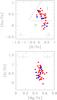 |
Fig. 3 Anti-correlations between light elements: Na-O (upper panel) and Mg-Al (lower panel). GIRAFFE stars are indicated by red filled circles and UVES stars by filled blue squares; upper limits in O are shown as arrows. The error bars are the cluster average internal (star-to-star) errors for each element for the GIRAFFE sample in red and UVES in blue (see text). In the upper panel we indicate the separation between P and I, and I and E populations, according to Carretta et al. (2009a). |
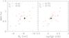 |
Fig. 4 Left panel: correlation between total absolute magnitude and the interquartile range of the [O/Na] ratio for GC in our FLAMES survey (Carretta et al. 2009a, 2010b, 2011a, 2013b, 2014b, 2015, and references therein). Right panel: relation between the maximum temperature along the HB (Recio-Blanco et al. 2006; Carretta et al. 2007) and IQR[O/Na]. In each panel NGC 6139 indicated by a filled green star. The Spearman rank correlation coefficient rs and the Pearson linear correlation coefficient rp are listed in each panel. |
Using the criteria defined in Carretta et al. (2009a), we can define the fraction of stars belonging to the primordial (P) and second-generation (I, E) components. The percentage of first-generation P stars is 26% ± 8%; the percentage of second-generation I stars (with moderate modification of the abundances) is 74% ± 13%; finally, there are no second-generation E stars (with extremely modified composition) in our sample of 43 stars in NGC 6139. These numbers agree with what is found in all massive Milky Way GCs (see, e.g., Carretta et al. 2010a, 2014b; Johnson & Pilachowski 2012, and references therein); SG stars are currently the dominant population in them. Our study then does not confirm NGC 6139 as a mainly-FG cluster, as proposed by Caloi & D’Antona (2011).
As for the other GCs in our sample (e.g., Carretta et al. 2009a), for which most of the abundance ratios are based on GIRAFFE spectra, the errors on abundances produce almost continuous distributions (Fig. 3). However, a separation between the P and I stars is visible in the upper panel (Na and O), especially for the stars observed with UVES. A clear-cut separation in groups along the Na-O anti correlation has only been seen in high-quality and high-resolution data, such as the UVES spectra in M4 (Marino et al. 2008) and NGC 2808 (Carretta 2014). The Mg-Al distribution (Fig. 3 lower panel) looks continuous, with a total excursion of about 1 dex in [Al/Fe].
The Na-O anti-correlation has moderate extension, with an interquartile range (IQR) for the [O/Na] ratio (Carretta 2006) IQR[O/Na] = 0.647. This IQR makes NGC 6139 fit in the relations with absolute magnitude (MV, i.e., mass) and maximum temperature reached on the HB ( (HB), Recio-Blanco et al. 2006; Carretta et al. 2007, see Fig. 4 for a graphical representation).
In conclusion, with our study of 45 member stars in NGC 6139 conducted with FLAMES spectra, we determined for the first time its metallicity with high-resolution spectroscopy (the cluster has an intermediate metallicity, with [Fe/H] = −1.58 dex). We also measured the light elements O, Na, Mg, and Al involved in proton-capture reactions of H-burning at high temperatures; we detected the usual correlations and anti-correlations found in almost all GCs investigated so far. The ratio of first-to-second generation stars in NGC 6139 is typical of the majority of GCs and is consistent with its relatively high total present-day mass. We do not support the idea that NGC 6139 is an FG-dominated cluster. The intermediate extension of the Na-O anti-correlation, as measured by the interquartile range of the [O/Na] ratio, fits the relation with the maximum temperature along the HB found by Carretta et al. (2007) very well. All in all, NGC 6139 behaves like a normal MW GC of similar mass and HB extension. The formation event that shaped its internal chemistry seems consistent with the pattern of a regular, relatively high-mass blue HB GC.
However, the finding of strong variation in Al, which should also imply some spread in He, does not perfectly agree with the HB of the cluster. We calculated IQR[Al/Mg], finding a value of 0.425; according to Fig. 28 in Gratton et al. (2010); this would require a ΔY of about 0.02 (but note that the relation between IQR[Al/Mg] and ΔY is rather poorly determined, being based on only eight points). We note also that the more massive, metal-poorer NGC 5024 (M53, with MV = −8.71, [Fe/H] =−2.10, Harris 1996), proposed to be an FG-dominated GC by Caloi & D’Antona (2011) on the basis of its HB and discussed at length in that paper, has been demonstrated to host a substantial SG by Mészáros et al. (2015), using APOGEE data. NGC 5024 has a wide spread in Al (with a bimodal distribution) and almost no Mg variation; it behaves like NGC 5272 (M3, MV = −8.88, [Fe/H] = −1.50, Harris 1996), another GC with a rather short HB, even more massive than NGC 6139, but with a similar metallicity. The relation between Al and He is evidently not completely understood. As as an additional cautionary note, Bastian et al. (2015) claimed that none of the enrichment mechanisms proposed to explain multiple populations in GCs can consistently do so, because all predict too wide He spreads to reproduce the observed spreads in light elements, notably those in Na and O. More observational constraints are required, both from spectroscopy with large samples of stars for which elements of all nucleosynthetic chains are measured (as we and other groups are doing for an increasing number of GCs) and from precise photometry (e.g., Piotto et al. 2015, to determine He). These constraints will be helpful in improving the modelling of the formation and early enrichment phases of GCs.
Online material
Appendix A: Additional tables
Information on the member stars observed.
Information on non-member stars on the basis of RV or metallicity, all observed with GIRAFFE.
Adopted atmospheric parameters and derived metallicity for confirmed member stars.
Light-element abundances for confirmed member stars.
This appears to occur, for instance, for NGC 6397 and NGC 6838 (Carretta et al. 2009b), for which Gratton et al. (2010) found that the He dispersion is not necessary to explain their HBs. However, Milone et al. (2012b) studied the main sequence of NGC 6397 and found an internal variation in Y of about 0.01, which is small, but exceeds their measurement error.
IRAF is distributed by the National Optical Astronomical Observatory, which are operated by the Association of Universities for Research in Astronomy, under contract with the National Science Foundation.
Harris (1996) refers to Webbink (1981), who used RVs from Kinman (1959), derived on spectra at R ~ 200 of four stars.
Acknowledgments
We thank the referee for constructive comments that improved the paper. This research has made use of WEBDA, SIMBAD database, operated at CDS, Strasbourg, France, and NASA’s Astrophysical Data System. This publication makes use of data products from the Two Micron All Sky Survey, which is a joint project of the University of Massachusetts and the Infrared Processing and Analysis Center/California Institute of Technology, funded by the National Aeronautics and Space Administration and the National Science Foundation. This research has been partially funded by PRIN INAF 2011 “Multiple populations in globular clusters: their role in the Galaxy assembly”, and PRIN MIUR 2010-2011, project “The Chemical and Dynamical Evolution of the Milky Way and Local Group Galaxies”.
References
- Alonso, A., Arribas, S., & Martínez-Roger, C. 1999, A&AS, 140, 261 [NASA ADS] [CrossRef] [EDP Sciences] [Google Scholar]
- Alonso, A., Arribas, S., & Martínez-Roger, C. 2001, A&A, 376, 1039 [NASA ADS] [CrossRef] [EDP Sciences] [Google Scholar]
- Bastian, N., Lamers, H. J. G. L. M., de Mink, S. E., et al. 2013, MNRAS, 436, 2398 [NASA ADS] [CrossRef] [MathSciNet] [Google Scholar]
- Bastian, N., Cabrera-Ziri, I., & Salaris, M. 2015, MNRAS, 449, 3333 [NASA ADS] [CrossRef] [Google Scholar]
- Boesgaard, A. M., Lum, M. G., & Deliyannis, C. P. 2015, ApJ, 799, 202 [Google Scholar]
- Bragaglia, A., Carretta, E., Gratton, R. G., et al. 2001, AJ, 121, 327 [NASA ADS] [CrossRef] [Google Scholar]
- Bragaglia, A., Gratton, R. G., Carretta, E., et al. 2012, A&A, 548, A122 [NASA ADS] [CrossRef] [EDP Sciences] [Google Scholar]
- Bragaglia, A., Sneden, C., Carretta, E., et al. 2014, ApJ, 796, 68 [NASA ADS] [CrossRef] [Google Scholar]
- Caloi, V., & D’Antona, F. 2011, MNRAS, 417, 228 [NASA ADS] [CrossRef] [Google Scholar]
- Cantat-Gaudin, T., Donati, P., Pancino, E., et al. 2014, A&A, 562, A10 [NASA ADS] [CrossRef] [EDP Sciences] [Google Scholar]
- Carretta, E. 2006, AJ, 131, 1766 [NASA ADS] [CrossRef] [Google Scholar]
- Carretta, E. 2014, ApJ, 795, L28 [NASA ADS] [CrossRef] [Google Scholar]
- Carretta, E., Recio-Blanco, A., Gratton, R. G., Piotto, G., & Bragaglia, A. 2007, ApJ, 671, L125 [NASA ADS] [CrossRef] [Google Scholar]
- Carretta, E., Bragaglia, A., Gratton, R. G., et al. 2009a, A&A, 505, 117 [NASA ADS] [CrossRef] [EDP Sciences] [Google Scholar]
- Carretta, E., Bragaglia, A., Gratton, R. G., & Lucatello, S. 2009b, A&A, 505, 139 [NASA ADS] [CrossRef] [EDP Sciences] [Google Scholar]
- Carretta, E., Bragaglia, A., Gratton, R. G., D’Orazi, V., & Lucatello, S. 2009c, A&A, 508, 695 [NASA ADS] [CrossRef] [EDP Sciences] [Google Scholar]
- Carretta, E., Bragaglia, A., Gratton, R. G., et al. 2010a, A&A, 516, A55 [NASA ADS] [CrossRef] [EDP Sciences] [Google Scholar]
- Carretta, E., Bragaglia, A., Gratton, R. G., et al. 2010b, A&A, 520, A95 [NASA ADS] [CrossRef] [EDP Sciences] [Google Scholar]
- Carretta, E., Lucatello, S., Gratton, R. G., Bragaglia, A., & D’Orazi, V. 2011a, A&A, 533, A69 [NASA ADS] [CrossRef] [EDP Sciences] [Google Scholar]
- Carretta, E., Bragaglia, A., Gratton, R., D’Orazi, V., & Lucatello, S. 2011b, A&A, 535, A121 [NASA ADS] [CrossRef] [EDP Sciences] [Google Scholar]
- Carretta, E., Bragaglia, A., Gratton, R. G., Lucatello, S., & D’Orazi, V. 2012, ApJ, 750, L14 [NASA ADS] [CrossRef] [Google Scholar]
- Carretta, E., Gratton, R. G., Bragaglia, A., D’Orazi, V., & Lucatello, S. 2013a, A&A, 550, A34 [NASA ADS] [CrossRef] [EDP Sciences] [Google Scholar]
- Carretta, E., Bragaglia, A., Gratton, R. G., et al. 2013b, A&A, 557, A138 [NASA ADS] [CrossRef] [EDP Sciences] [Google Scholar]
- Carretta, E., Bragaglia, A., Gratton, R. G., et al. 2014a, A&A, 561, A87 [NASA ADS] [CrossRef] [EDP Sciences] [Google Scholar]
- Carretta, E., Bragaglia, A., Gratton, R. G., et al. 2014b, A&A, 564, A60 [NASA ADS] [CrossRef] [EDP Sciences] [Google Scholar]
- Carretta, E., Bragaglia, A., Gratton, R. G., et al. 2015, A&A, 578, A116 [NASA ADS] [CrossRef] [EDP Sciences] [Google Scholar]
- Cohen, J. G. 2004, AJ, 127, 1545 [NASA ADS] [CrossRef] [Google Scholar]
- Cunha, K., Smith, V. V., Johnson, J. A., et al. 2015, ApJ, 798, L41 [NASA ADS] [CrossRef] [MathSciNet] [Google Scholar]
- D’Antona, F., Bellazzini, M., Caloi, V., et al. 2005, ApJ, 631, 868 [NASA ADS] [CrossRef] [Google Scholar]
- D’Antona, F., Caloi, V., D’Ercole, A., et al. 2013, MNRAS, 434, 1138 [NASA ADS] [CrossRef] [Google Scholar]
- Davidge, T. J. 1998, AJ, 116, 1744 [NASA ADS] [CrossRef] [Google Scholar]
- Decressin, T., Meynet, G., Charbonnel, C., Prantzos, N., & Ekström, S. 2007, A&A, 464, 1029 [NASA ADS] [CrossRef] [EDP Sciences] [Google Scholar]
- Geisler, D., Villanova, S., Carraro, G., et al. 2012, ApJ, 756, L40 [NASA ADS] [CrossRef] [Google Scholar]
- de Silva, G. M., Gibson, B. K., Lattanzio, J., & Asplund, M. 2009, A&A, 500, L25 [NASA ADS] [CrossRef] [EDP Sciences] [MathSciNet] [Google Scholar]
- Gratton, R. G. 1988, Rome Obs. Preprint Ser., 29 [Google Scholar]
- Gratton, R. G., Carretta, E., Eriksson, K., & Gustafsson, B. 1999, A&A, 350, 955 [NASA ADS] [Google Scholar]
- Gratton, R. G., Carretta, E., Claudi, R., Lucatello, S., & Barbieri, M. 2003, A&A, 404, 187 [NASA ADS] [CrossRef] [EDP Sciences] [Google Scholar]
- Gratton, R., Sneden, C., & Carretta, E. 2004, ARA&A, 42, 385 [NASA ADS] [CrossRef] [Google Scholar]
- Gratton, R. G., Lucatello, S., Bragaglia, A., et al. 2007, A&A, 464, 953 [NASA ADS] [CrossRef] [EDP Sciences] [Google Scholar]
- Gratton, R. G., Carretta, E., Bragaglia, A., Lucatello, S., & D’Orazi, V. 2010, A&A, 517, A81 [NASA ADS] [CrossRef] [EDP Sciences] [Google Scholar]
- Gratton, R. G., Carretta, E., & Bragaglia, A. 2012, A&ARv, 20, 50 [CrossRef] [Google Scholar]
- Harris, W. E. 1996, AJ, 112, 1487 [NASA ADS] [CrossRef] [Google Scholar]
- Hazen, M. L. 1991, AJ, 101, 170 [NASA ADS] [CrossRef] [Google Scholar]
- Johnson, C. I., & Pilachowski, C. A. 2012, ApJ, 754, L38 [NASA ADS] [CrossRef] [Google Scholar]
- Johnson, J. A., Ivans, I. I., & Stetson, P. B. 2006, ApJ, 640, 801 [NASA ADS] [CrossRef] [Google Scholar]
- Kinman, T. D. 1959, MNRAS, 119, 157 [NASA ADS] [Google Scholar]
- Kurucz, R. 1993, ATLAS9 Stellar Atmosphere Programs and 2 km s-1 grid, CD-ROM No. 13 (Cambridge, Mass.: Smithsonian Astrophysical Observatory) [Google Scholar]
- Larsen, S. S., Strader, J., & Brodie, J. P. 2012, A&A, 544, L14 [NASA ADS] [CrossRef] [EDP Sciences] [Google Scholar]
- Letarte, B., Hill, V., Jablonka, P., et al. 2006, A&A, 453, 547 [NASA ADS] [CrossRef] [EDP Sciences] [Google Scholar]
- MacLean, B. T., De Silva, G. M., & Lattanzio, J. 2014, MNRAS, 466, 3556 [Google Scholar]
- Magain, P. 1984, A&A, 134, 189 [NASA ADS] [Google Scholar]
- Marino, A. F., Villanova, S., Piotto, G., et al. 2008, A&A, 490, 625 [NASA ADS] [CrossRef] [EDP Sciences] [Google Scholar]
- Mészáros, S., Martell, S. L., Shetrone, M., et al. 2015, AJ, 149, 153 [NASA ADS] [CrossRef] [Google Scholar]
- Milone, A. P., Piotto, G., Bedin, L. R., et al. 2012a, ApJ, 744, 58 [NASA ADS] [CrossRef] [Google Scholar]
- Milone, A. P., Marino, A. F., Piotto, G., et al. 2012b, ApJ, 745, 27 [NASA ADS] [CrossRef] [Google Scholar]
- Milone, A. P., Marino, A. F., Dotter, A., et al. 2014, ApJ, 785, 21 [NASA ADS] [CrossRef] [Google Scholar]
- Mucciarelli, A., Origlia, L., Ferraro, F. R., & Pancino, E. 2009, ApJ, 695, L134 [NASA ADS] [CrossRef] [Google Scholar]
- Nataf, D. M., Gould, A. P., Pinsonneault, M. H., & Udalski, A. 2013, ApJ, 766, 77 [NASA ADS] [CrossRef] [Google Scholar]
- Ortolani, S., Bica, E., & Barbuy, B. 1999, A&AS, 138, 267 [NASA ADS] [CrossRef] [EDP Sciences] [Google Scholar]
- Pasquini, L., Avila, G., Blecha, A., et al. 2002, The Messenger, 110, 1 [NASA ADS] [Google Scholar]
- Piotto, G., King, I. R., Djorgovski, S. G., et al. 2002, A&A, 391, 945 [NASA ADS] [CrossRef] [EDP Sciences] [Google Scholar]
- Piotto, G., Bedin, L. R., Anderson, J., et al. 2007, ApJ, 661, L53 [NASA ADS] [CrossRef] [Google Scholar]
- Piotto, G., Milone, A. P., Bedin, L. R., et al. 2015, AJ, 149, 91 [NASA ADS] [CrossRef] [Google Scholar]
- Prantzos, N., Charbonnel, C., & Iliadis, C. 2007, A&A, 470, 179 [NASA ADS] [CrossRef] [EDP Sciences] [Google Scholar]
- Recio-Blanco, A., Aparicio, A., Piotto, G., de Angeli, F., & Djorgovski, S. G. 2006, A&A, 452, 875 [NASA ADS] [CrossRef] [EDP Sciences] [Google Scholar]
- Samus’, N. N., Kravtsov, V. V., Pavlov, M. V., et al. 1996, Astron. Lett., 22, 686 [NASA ADS] [Google Scholar]
- Saviane, I., da Costa, G. S., Held, E. V., et al. 2012, A&A, 540, A27 [NASA ADS] [CrossRef] [EDP Sciences] [Google Scholar]
- Sbordone, L., Bonifacio, P., Buonanno, R., et al. 2007, A&A, 465, 815 [NASA ADS] [CrossRef] [EDP Sciences] [Google Scholar]
- Sbordone, L., Salaris, M., Weiss, A., & Cassisi, S. 2011, A&A, 534, A9 [NASA ADS] [CrossRef] [EDP Sciences] [Google Scholar]
- Skrutskie, M. F., Cutri, R. M., Stiening, R., et al. 2006, AJ, 131, 1163 [NASA ADS] [CrossRef] [Google Scholar]
- Stetson, P. B. 1987, PASP, 99, 191 [NASA ADS] [CrossRef] [Google Scholar]
- Stetson, P. B. 1993, in Stellar photometry – Current techniques and future developments, eds. C. J. Butler, & I. Elliott (Cambridge: Cambridge Univ. Press), Proc. IAU Colloq., 136, 291 [Google Scholar]
- Stetson, P. B., & Pancino, E. 2008, PASP, 120, 1332 [Google Scholar]
- Tautvaišienė, G., Wallerstein, G., Geisler, D., Gonzalez, G., & Charbonnel, C. 2004, AJ, 127, 373 [NASA ADS] [CrossRef] [Google Scholar]
- Ventura, P., D’Antona, F., Mazzitelli, I., & Gratton, R. 2001, ApJ, 550, L65 [NASA ADS] [CrossRef] [Google Scholar]
- Villanova, S., Geisler, D., Carraro, G., Moni Bidin, C., & Muñoz, C. 2013, ApJ, 778, 186 [NASA ADS] [CrossRef] [Google Scholar]
- Webbink, R. F. 1981, ApJS, 45, 259 [NASA ADS] [CrossRef] [Google Scholar]
- Zinn, R., & Barnes, S. 1998, AJ, 116, 1736 [NASA ADS] [CrossRef] [Google Scholar]
All Tables
Sensitivities of abundance ratios to variations in the atmospheric parameters and to errors in the equivalent widths, and errors in abundances for stars of NGC 6139 observed with UVES.
Sensitivities of abundance ratios to variations in the atmospheric parameters and to errors in the equivalent widths, and errors in abundances for stars of NGC 6139 observed with GIRAFFE.
Information on non-member stars on the basis of RV or metallicity, all observed with GIRAFFE.
Adopted atmospheric parameters and derived metallicity for confirmed member stars.
All Figures
|
Fig. 1 a) CMD of NGC 6139, with its quite short blue HB. In grey we plot all stars, in red all targets observed with FLAMES. The seven UVES stars are indicated by blue open squares; the stars with RV from Saviane et al. (2012) are represented by blue crosses. b) The non-member stars (and the star on the HB) are indicated by red open squares, the stars that are candidate members on the basis of their RV by filled blue squares. The member stars define a reasonably tight RGB, and we indicate with green circles the probable AGB stars (see Sect. 3.1) |
| In the text | |
|
Fig. 2 Upper panel: histogram of all measured RVs (open histogram) and of the candidate member stars alone (blue filled histogram). Lower panel: RVs versus distance from the cluster centre. The candidate member stars are indicated by filled blue squares, the UVES targets by large red crosses, and the lines indicate the cluster mean RV and the ± 3σ interval. |
| In the text | |
|
Fig. 3 Anti-correlations between light elements: Na-O (upper panel) and Mg-Al (lower panel). GIRAFFE stars are indicated by red filled circles and UVES stars by filled blue squares; upper limits in O are shown as arrows. The error bars are the cluster average internal (star-to-star) errors for each element for the GIRAFFE sample in red and UVES in blue (see text). In the upper panel we indicate the separation between P and I, and I and E populations, according to Carretta et al. (2009a). |
| In the text | |
|
Fig. 4 Left panel: correlation between total absolute magnitude and the interquartile range of the [O/Na] ratio for GC in our FLAMES survey (Carretta et al. 2009a, 2010b, 2011a, 2013b, 2014b, 2015, and references therein). Right panel: relation between the maximum temperature along the HB (Recio-Blanco et al. 2006; Carretta et al. 2007) and IQR[O/Na]. In each panel NGC 6139 indicated by a filled green star. The Spearman rank correlation coefficient rs and the Pearson linear correlation coefficient rp are listed in each panel. |
| In the text | |
Current usage metrics show cumulative count of Article Views (full-text article views including HTML views, PDF and ePub downloads, according to the available data) and Abstracts Views on Vision4Press platform.
Data correspond to usage on the plateform after 2015. The current usage metrics is available 48-96 hours after online publication and is updated daily on week days.
Initial download of the metrics may take a while.