| Issue |
A&A
Volume 583, November 2015
Rosetta mission results pre-perihelion
|
|
|---|---|---|
| Article Number | A24 | |
| Number of page(s) | 6 | |
| Section | Planets and planetary systems | |
| DOI | https://doi.org/10.1051/0004-6361/201526351 | |
| Published online | 30 October 2015 | |
Suprathermal electron environment of comet 67P/Churyumov-Gerasimenko: Observations from the Rosetta Ion and Electron Sensor
1 The Catholic University of America, Washington, DC 20064, USA
2 NASA Goddard Space Flight Center, Greenbelt, MD 20771, USA
3 Space Science and Engineering Division, Southwest Research Institute, San Antonio, TX 78249, USA
4 Department of Physics and Astronomy, University of Kansas, Lawrence, KS 66045, USA
5 Department of Physics and Astronomy, University of Texas at San Antonio, San Antonio, TX 78249, USA
Received: 18 April 2015
Accepted: 15 May 2015
Abstract
Context. The Rosetta spacecraft is currently escorting comet 67P/Churyumov-Gerasimenko until its perihelion approach at 1.2 AU. This mission has provided unprecedented views into the interaction of the solar wind and the comet as a function of heliocentric distance.
Aims. We study the interaction of the solar wind and comet at large heliocentric distances (>2 AU) using data from the Rosetta Plasma Consortium Ion and Electron Sensor (RPC-IES). From this we gain insight into the suprathermal electron distribution, which plays an important role in electron-neutral chemistry and dust grain charging.
Methods. Electron velocity distribution functions observed by IES fit to functions used to previously characterize the suprathermal electrons at comets and interplanetary shocks. We used the fitting results and searched for trends as a function of cometocentric and heliocentric distance.
Results. We find that interaction of the solar wind with this comet is highly turbulent and stronger than expected based on historical studies, especially for this weakly outgassing comet. The presence of highly dynamical suprathermal electrons is consistent with observations of comets (e.g., Giacobinni-Zinner, Grigg-Skjellerup) near 1 AU with higher outgassing rates. However, comet 67P/Churyumov-Gerasimenko is much farther from the Sun and appears to lack an upstream bow shock.
Conclusions. The mass loading process, which likely is the cause of these processes, plays a stronger role at large distances from the Sun than previously expected. We discuss the possible mechanisms that most likely are responsible for this acceleration: heating by waves generated by the pick-up ion instability, and the admixture of cometary photoelectrons.
Key words: comets: individual: 67P/Churyumov-Gerasimenko / plasmas / solar wind
Now at Johns Hopkins University Applied Physics Laboratory, Laurel, MD, USA, e-mail: This email address is being protected from spambots. You need JavaScript enabled to view it.
© ESO, 2015
1. Introduction
The solar wind interaction with a comet has been studied with great interest for the past several decades and much of our knowledge is based on the in situ plasma measurements from the past thirty years (e.g. Bame et al. 1986; Haerendel et al. 1986; Coates et al. 1987; Cravens et al. 1987). These in situ measurements have been limited to flybys when the comets were close to their perihelion approach (~1 AU). Consequently, many questions still remain open about solar wind interaction with comets. An important process that we discuss in this paper is the mass loading process. Mass loading occurs when the gases in the cometary coma are photoionized (from solar extreme ultraviolet radiation, EUV) and thus can now interact with the solar wind flow by being picked up in the interplanetary magnetic field (IMF). A comprehensive review of this process can be found in Szego et al. (2000). When enough mass is added to the solar wind flow, it becomes significantly decelerated, which causes magnetic field pile-up regions to occur, and a bow shock upstream of the comet may be produced. Qualitatively, the dynamics of this shock region can resemble the structure and dynamics observed at planetary bow shocks; quantitatively, however, the two regimes are significantly different. For example, in the cometary plasma environment, gyro-radii can be much larger than the comet itself and its gravitationally unbound neutral coma. In this scenario particle motions become important, and it requires a kinetic approach. In contrast, the fluid approach in planetary magnetospheres (e.g. Earth) works well. Comparative studies between these very different plasma environments can reveal new and interesting physics.
It is not surprising that the mass loading process is strongly coupled to the neutral content and thus to the outgassing rate of the comet (Szego et al. 2000). Furthermore, comparative studies between cometary electron plasma environments paint a different picture, which has been linked to the total outgassing rate (Reme et al. 1993). One particular feature that appears to be linked to the outgassing rate is the characteristics of suprathermal electrons. Suprathermal electrons are accelerated by an unknown mechanism from a few eV upward to 100 s of eV and play an important role in the electron-neutral chemistry as well as in dust grain charging (Cravens et al. 1987; Mendis & Horányi 2013; Gombosi et al. 2015). Previous works (Thomsen et al. 1986; Reme et al. 1993; Bingham et al. 1988; Hall et al. 1986), all showed that accelerated electrons are ubiquitous in the interaction of the solar wind with the comet (or pseudo-comet in the case of Bingham et al. 1988; Hall et al. 1986), but these works also postulated different dominant mechanisms. For example, Thomsen et al. (1986) showed that accelerated electrons (< ~ 200 eV) at comet Giacobinni-Zinner (G-Z) were likely associated with upstream wave fluctuations convecting tailward. The high degree of variability in their observations led the authors to assume that a weakly, intermittent shock resided upstream. They also found that their results compared well with electron spectra accelerated behind interplanetary collisionless shocks (Feldman et al. 1983b). A comparative study by Reme et al. (1993) also showed that large modulations in the electron fluxes (100 s of eV) existed in measurements of the cometosheath of comet Grigg-Skjellerup (G-S). In the same study, they showed comet Halley to have more coherent structures and linked to differences in the gas production rate. The Active Magnetospheric Particle Tracer Explorers (AMPTE) satellite studied the effects of the solar wind interacting with a pseudo-comet generated by the release of barium ions (Haerendel et al. 1986). Results from AMPTE showed that electrons were mainly accelerated by lower hybrid waves generated by the pick-up ion process (Bingham et al. 1988; Hall et al. 1986). A review of cometary pick-up ions and their effects on the local plasma environment can be found in (Coates 2004, and references therein). Other work, such as (e.g. Gan & Cravens 1990) suggested that photoelectrons play an important role in the electron energetics, where, as other studies claim, it is negligible (Hall et al. 1986). It is clear from the literature that cometary environments can drastically differ from one another, with several different processes at play to varying degrees.
Since 2014, the Rosetta spacecraft has escorted comet 67P/Churyumov-Gerasimenko (comet 67P) on its trajectory through the inner solar system, thus providing the first continuous observations of the interaction of solar wind and comet. For context, the outgassing rate of comet 67P is approximately 100 times lower than that of comet Halley and ten times lower than that of comet Giacobinni-Zinner (G-Z). The initial rendezvous with comet 67P occurred at a heliocentric distance of ~3.6 AU, a point in space and time where most models predicted a very weak interaction with the solar wind (Mendis & Horányi 2014; Koenders et al. 2013). This is well-founded based on the knowledge of cometary flybys near 1 AU (a time of peak cometary activity). In this paper, we present suprathermal electron measurements from the Rosetta Ion and Electron Sensor (IES; Burch et al. 2007) that contradict previous expectations and show a rich and dynamic electron environment. We conclude that the role of mass loading beyond 3 AU is still significant, even for weakly outgassing comets such as comet 67P. We also consider possible mechanisms of energizing the electrons at 67P and compare them with previous observations from comet flybys and cometary plasma modeling.
2. Instrument and data
The Rosetta IES is a toroidal top hat electrostatic analyzer that measures the 3D fluxes of ions and electrons over an energy-per-charge (E/q) from 4 eV/q to 17 keV/q with an energy resolution of 8%. IES has a 360° field of view (FOV) in the symmetry plane and is swept electrostatically in elevation + / − 45° normal to that plane in 16 different angles, about 5.5°. The electron sensor has 16 discrete anodes with a FWHM angular resolution of 22.5°. A 3D distribution typically takes 128 seconds to complete. Several data modes are used in flight. Time multipliers and angular integration are mode dependent. These nuances are taken into account when analyzing the raw data. IES is mounted on the top corner of the spacecraft science deck and allows simultaneous viewing of the comet and solar wind under most orbital conditions. However, there are still parts of the IES FOV that are occulted by spacecraft structures and various instruments. These blockages are illustrated in Fig. 1. Vertical and horizontal axes represent the IES elevation and azimuthal look directions. The segmented boxes on the horizontal axis refer to the electron (top) and ion (bottom) anode numbering scheme. These blockages inhibit particle measurements and need to be carefully taken into account. The spacecraft potential can also inhibit the measurements by linearly shifting their observed energy distribution. The Rosetta Langmuir Probe (LAP) team has observed primarily negative spacecraft potentials (Anders Eriksson, private communication). Effectively, this translates into part of the low-energy electron distribution being repelled, thus IES does not observe the full electron phase space density. However, this does not significantly affect the suprathermal electrons.
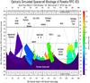 |
Fig. 1 Various components of the Rosetta spacecraft and its instrumentation are coded in different colors to show obstructions in the IES view field. IES ion anode numbers are shown in segments between 85° − 90° and −85° − −90°. IES electron anode numbers are shown in segments between 80° − 85° and −80° − −85°. The solar array, high-gain antenna, and ROSINA RTOF cap are all moving within the IES view field. |
Rosetta rendezvoused with comet 67P in August 2014 at a heliocentric distance of ~3.6 AU. For the period considered in this study, Rosetta has gone into a terminator-like orbit and has been monitoring the comet continuously with varying radial distances between ~10 km to ~50 km. Rosetta has an orbital velocity relative to the comet of ~1 m/s. At the time of writing (February 2015), the comet has traversed over 1 AU and is now at a distance of ~2.4 AU from the Sun. Figure 2 depicts Rosetta’s trajectory in comet solar ecliptic (CSO) coordinates. Darker shades of blue represent elapsed time.
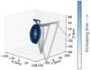 |
Fig. 2 Rosetta’s trajectory from August 2014 until January 2015 (the time frame considered in this study). Elapsed time is illustrated by a darker shade of blue in the color bar. |
3. Electron observations
Rosetta IES observations of the electrons depict a dynamical environment, which can be seen in Fig. 3. During the early phases of the capture orbit the electrons exhibited a typical solar wind-like spectrum. This spectrum which can be characterized by bi-Maxwellian distributions (Pilipp et al. 1987). As Rosetta approached 67P and began a terminator orbit only tens of km distant from the nucleus (August 2014, top panel), the electrons were accelerated to several tens or hundreds of eV. Subsequently (September 2014 and thereafter), Rosetta IES observed dynamical electron signatures that varied in time and energy; it is all shown in the montage of energy-per-charge signatures from August to January in Fig. 3. Qualitatively, from visual inspection, the suprathermal electrons are consistently accelerated to higher energies with time (or with heliocentric distance); this is also shown quantitatively in Fig. 5. The Rosetta terminator orbit varies only slowly with time (1 m/s relative velocity) and does not change significantly from orbit to orbit. Furthermore, electron gyroradii are similar to the radial distance variation observed during the first several months of observations. For example, a 100 eV electron in a 2 nT field has a gyroradius of ~17 km. We note that some features in the data are not purely due to typical solar wind plasma impinging on the neutral coma of 67P – some features (possibly interplanetary shocks) are known and are represented by the white arrows in Fig. 3. This may not be a comprehensive list to date. IES mode-dependent features can sometimes be seen as data gaps at energies >1 keV; they also sometimes produce a smearing effect or portray elevated background counts (e.g., see 11/19 in Fig. 3). Other examples of data gaps occurred when IES was turned off (e.g., see 9/2-9/4 in Fig. 3).
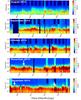 |
Fig. 3 Electron energy versus time spectrograms (q = 1 for electrons) from August 2014 until January 2015. Colors represent logarithmic counts per second. White arrows represent times when solar wind structures (e.g. CIRs) are thought to be present. |
The suprathermal electrons (~10−300 eV) are not Maxwellian. We therefore fit the suprathermal component of the electron distribution using (Thomsen et al. 1986; Feldman et al. 1983b,a; Dum et al. 1974) ![Mathematical equation: \begin{equation} f(v)=A \exp{[-(v/v_{\rm o})^{p}]} \end{equation}](/articles/aa/full_html/2015/11/aa26351-15/aa26351-15-eq14.png) (1)where A is the amplitude, v is the velocity, vo is related to the temperature of the electron distribution and p is the power. The shape and evolution of the suprathermal electrons (~10−300 eV) are characterized from the Rosetta rendezvous until the end of January. Figure 4 illustrates three examples of electron velocity distribution functions (VDFs) from comet 67P: (1) a solar wind distribution taken nearly 120 km upstream of the comet at a heliocentric distance of ~3.6 AU (blue curve); (2) electrons that are energized to ~60 eV (black curve); and (3) electrons that are energized to ~100 eV (green curve). The energized distributions (2 and 3) were recorded at cometocentric distances of ~50 km and 10 km or heliocentric distances of ~3.3 AU and ~3 AU, respectively. The red curves in Fig. 4 are fits from Eq. (1) to the energized VDFs (2 and 3). The generalized Gaussian (Eq. (1)) has two free parameters, vo and p, which were determined through a nonlinear least-squares fitting routine. The shape and peaks of the electron distributions are consistent with those reported by Thomsen et al. (1986) and Hall et al. (1986). The narrow or broad shoulders of the suprathermal component are captured by the power p in Eq. (1) – higher values of p represent a more flat-top distribution with a sharply decreasing slope with velocity. In contrast, lower values of p represent broader shoulders (more electrons are energized to higher energies). A suprathermal distribution best fit with p ≈ 2 can also be represented by a Maxwellian distribution. Above a few hundred electron volts, the remaining high-energy tail can be characterized by a Maxwellian and a power law distribution. We focus on the part of the distribution that can be characterized by Eq. (1), namely ~10 eV to 200 eV. The one-count level is shown as the green dashed curved. The electron spectra in Fig. 4 show evidence of energy-dependent acceleration, which we discuss in more detail in Sect. 4.
(1)where A is the amplitude, v is the velocity, vo is related to the temperature of the electron distribution and p is the power. The shape and evolution of the suprathermal electrons (~10−300 eV) are characterized from the Rosetta rendezvous until the end of January. Figure 4 illustrates three examples of electron velocity distribution functions (VDFs) from comet 67P: (1) a solar wind distribution taken nearly 120 km upstream of the comet at a heliocentric distance of ~3.6 AU (blue curve); (2) electrons that are energized to ~60 eV (black curve); and (3) electrons that are energized to ~100 eV (green curve). The energized distributions (2 and 3) were recorded at cometocentric distances of ~50 km and 10 km or heliocentric distances of ~3.3 AU and ~3 AU, respectively. The red curves in Fig. 4 are fits from Eq. (1) to the energized VDFs (2 and 3). The generalized Gaussian (Eq. (1)) has two free parameters, vo and p, which were determined through a nonlinear least-squares fitting routine. The shape and peaks of the electron distributions are consistent with those reported by Thomsen et al. (1986) and Hall et al. (1986). The narrow or broad shoulders of the suprathermal component are captured by the power p in Eq. (1) – higher values of p represent a more flat-top distribution with a sharply decreasing slope with velocity. In contrast, lower values of p represent broader shoulders (more electrons are energized to higher energies). A suprathermal distribution best fit with p ≈ 2 can also be represented by a Maxwellian distribution. Above a few hundred electron volts, the remaining high-energy tail can be characterized by a Maxwellian and a power law distribution. We focus on the part of the distribution that can be characterized by Eq. (1), namely ~10 eV to 200 eV. The one-count level is shown as the green dashed curved. The electron spectra in Fig. 4 show evidence of energy-dependent acceleration, which we discuss in more detail in Sect. 4.
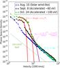 |
Fig. 4 Electron velocity distribution functions. Representative VDF for the evolution from a solar wind-like VDF (blue curve) to accelerated VDFs (black and green curves). A generalized Gaussian (Eq. (1)) is used to fit the non-Maxwellian suprathermal distribution. At high electron velocities, the distribution resembles a Maxwellian part and then a power-law dependence (purple and cyan curves). Error bars are reported (Poisson statistics), but they are smaller than the marker size. |
Rosetta IES electron measurements between August 2014 and January 2015 were fitted to the generalized Gaussian and the free fitting parameters p and vo were recorded for each fit. We note that the fitting routine did not converge for every measured distribution; we leave this for further investigation. Figure 5a illustrates p as a function of heliocentric distance. The data were binned into 0.1 AU bins; error bars represent the variance and the solid black line represents the mean. The mean value of p shows a decreasing trend as the comet approaches perihelion. This means that acceleration becomes stronger. It is expected that the outgassing rate increases as the comet approaches the Sun. This leads to an increase in ionization and mass loading, which may be controlling the dynamics of the suprathermal population. However, the variance in p remains similar perhaps suggesting a dynamic acceleration mechanism. Figure 5b shows the number of events in each bin that were used to determine the mean and variance of p. The large variation in the shape of the suprathermal electron distribution was also observed by Thomsen et al. (1986) at comet G-Z. They postulated that the variations were due to fluctuations in the upstream conditions and that depending on the upstream plasma, the shock may decay altogether, thus leading to variably shocked plasma regions. Their observations were also made at a heliocentric distance of ~1 AU and the outgassing rate of G-Z is approximately a factor 10 higher than predicted for comet 67P. In contrast, modulations in the observed electron flux at comet Halley were much weaker (Reme et al. 1993). It is surprising that a weakly outgassing comet at large heliocentric distances produces a dynamic and energetic suprathermal electron environment. We discuss this in more detail in the next section.
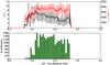 |
Fig. 5 Mean values for the free fitting parameters from Eq. (1) as a function of heliocentric distance (top panel). Total number of events in each 0.1 AU bin (bottom panel). Error bars are represented by the variance in each parameter. |
The fitting parameters p and vo were mapped out along the spacecraft trajectory in the comet centered solar orbit (CSO). In the CSO frame, x points toward the Sun, y is the component of the comet velocity vector orthogonal to x, and z completes the right-handed reference frame. The results are illustrated in Fig. 6. Panel a shows the p values in the z-y plane, and panels b, c, and d are collapsed to the z, y, and x plane, respectively. These data were spatially binned in 0.5 km bins. Unlike Fig. 5, where the mean value of p appears connected to heliocentric distance, there is no clear organization in the cometocentric frame. This may be because the S/C orbit is mainly located along the terminator orbit in this study or because the mechanism responsible for energizing the electrons is active over a large spatial scale around the comet. The variance in p is also significantly stronger. On shorter time scales, variations in the electron environment appear to be qualitatively correlated with factors that control the sources of neutral gas (i.e., rotation, latitude, etc.).
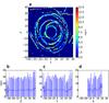 |
Fig. 6 Mean value of p (see Eq. (1)) mapped along Rosetta’s trajectory in the CSO frame for the Z-Y plane (see text for definitions). Panels b), c), and d) are cuts through the z, y, and x plane respectively. Error bars represent the variance of p. Bins are 0.5 km in width. |
4. Discussion
Comet 67P is a weakly outgassing comet (a factor of 10 lower than G-Z and a factor of 100 lower than Halley); even at large heliocentric distances (≥3 AU), however, IES observes a rich and dynamic suprathermal electron environment. Electron VDFs measured by IES exhibit features that are consistent with previous electron acceleration studies (Thomsen et al. 1986; Feldman et al. 1983b; Hall et al. 1986; Bingham et al. 1988). Table 1 summarizes the values of p found in this study and previous works. Here, we briefly introduce the various mechanisms that have been shown to accelerate electrons and discuss the context of our observations.
Values of p found in different physical environments.
4.1. Mixing of photoelectrons, secondaries and the solar wind
Photoelectrons are created through the interaction of a solar EUV photon and neutral molecule in the coma. The resulting energy of a photoelectron depends on the ionization potential and results in discrete energy peaks. Secondaries are created through the interaction of an energetic electron with a neutral molecule and have energies equal to the electron incident energy minus the molecule’s ionization potential. These processes have been shown to play an important role in shaping the electron spectra at comets (Cravens et al. 1987, and references therein). Another study (Hall et al. 1986) has shown photoelectrons to play an insignificant role in the accelerated electron spectra. The unperturbed densities from both of these sources near the nucleus are lower than 1 cm3, yet the observed electron densities are closer to 10 − 100 cm3. Which processes account for the density (and flux) enhancements that IES observes are not obvious, but may involve the ambipolar electric field and/or a local compression in the flow. The ambipolar electric field is proportional to the electron pressure gradient and is required to maintain quasi-neutrality with significant ion densities being produced by photoionization (e.g. Cravens, in prep.). Any mechanism (e.g., electrostatic fields) must have some degree of structure to account for the large variations in the energies and fluxes seen on short time-scales. The observed VDFs show no evidence of a clear peak (a maximum with positive and negative slopes on either side) in phase space, either. This typically is a distribution that has a flat top or broad shoulder and rolls off with increasing energy. If a well-structured electric field were present, then a well-defined peak would be expected. Again, this points to fine structure in the plasma environment. It might likewise be important that comet 67P is dominated by kinetic processes.
4.2. Electrostatic shock potentials
Cross-shock potentials have been observed to accelerate electrons to energies of 100 s of eV (e.g. Feldman et al. 1983b). Some of the electron VDFs we presented here resemble a flat top-like distribution, similar to those seen at Earth’s bow shock. The p values we reported are also consistent with those observed by Feldman et al. (1983b). However, no evidence exists that would show comet 67P to develop a bow shock as far out as ~3.5 AU, when IES first started to observe these accelerated electrons. Moreover, for the time frame considered here, the ion data do not show a significant deceleration of the solar wind, which one might expect if a bow shock existed. Lastly, magnetic field data have not shown any evidence of a reverse shock, which is associated with cometary bow shocks. Consequently, we postulate that these signatures are probably no caused by an upstream bow shock.
4.3. Magnetic field compression
Compression of the magnetic field leads to adiabatic energization through conservation of the first invariant. This mechanism leads to an increase in perpendicular (to the magnetic field) energy. Unfortunately, the magnetic field magnitude and direction are not available at this time. However, we observe changes on orders of magnitude and larger in the count rate on short time-scales. This would suggest that the magnetic field compressions are equally as large and rapidly changing, which is unlikely. This process undoubtedly plays a role, but it probably is not the dominant mechanism accelerating the electrons.
4.4. Wave-particle interactions
One common feature associated with the works of Thomsen et al. (1986), Hall et al. (1986), Bingham et al. (1988), and Reme et al. (1993) is the role of electromagnetic waves. The pick-up ion process creates a source of free energy that can be easy transmitted through waves to the electrons. Shapiro et al. (1999) considered the role of lower hybrid waves in accelerating electrons in cometary environments. They used a modified two-stream instability (MTSI) of the different ion population resulting from mass loading between the solar wind and cometary coma. By balancing the growth rate of lower hybrid waves with the Landau damping rate of electrons that is due to the interaction, they produced an effective average energy and density of the suprathermal electrons resulting from this process (Shapiro et al. 1999, cf. Eq. (22)). They found that at comet Hyakutake the average energy of the suprathermal electrons is ~100 eV with a density of ~5−10 cm-3. The outgassing rate of comet Hyakutake’s outgassing rate was estimated to be 6 − 10 × 1028 mol/s at 1 AU. They predicted that the suprathermal electron density scales with the cometary ion density. The energy and density of electrons energized through lower hybrid waves appears to be consistent with our observations. Using data from the Ion Composition Analyzer (ICA), Nilsson et al. (2015) performed a statistical analysis of the ion environment between 2.0 and 3.6 AU. Their work illustrates that the comet becomes more active through showing the increased flux in water pick-up ions as a function of heliocentric distance (Nilsson et al. 2015, cf. Fig. 3). We note that the accelerated water ion fluxes reported by Nilsson et al. (2015) match our results well (see Fig. 5 in this paper). An analysis of pick-up ion distributions around comet 67P was also reported by Goldstein et al. (2015) and Broiles et al. (2015). Lower hybrid wave frequencies have frequencies between that of the electron and proton gyrofrequency. Unfortunately, there is no instrument onboard Rosetta that can measure electromagnetic waves at this frequency.
4.5. Prospects
Rosetta will soon transition from the terminator-like orbit and perform flybys with varying apogees, while also continuing to escort the comet through the inner solar system with a perihelion approach in early August 2015 at ~1.2 AU. The gas production rate is expected to increase, and mass loading will become more significant. Currently, Rosetta is scheduled for an excursion that will take it out to 1500 km, which will give an unprecedented view on the spatial variability of the plasma. These future anticipated measurements will complement this study and provide observations on the strength and variability of the suprathermal electrons far from the comet. Modeling endeavors of the plasma environment should aim at reproducing the low-to mid-energy spectral shapes reported here. Our results also suggest that the electron signatures are probably not due to latitudinal or longitudinal differences in the orbit, but rather are a function of heliocentric distance. Finally, because we do not yet know the magnetic field direction, we were unable to investigate anisotropies with respect to the magnetic field. Deeper insight into the acceleration processes will be gained by case studies from which detailed information about the IMF direction can be inferred.
5. Summary
We presented the first assessment of electron observations from Rosetta IES. We found that electrons are being accelerated upward to several hundreds of eV, which is most likely due to an admixture of photoelectrons and waves produced by the pick-up ion instability. Cross-shock potentials and adiabatic compression acting as a dominant acceleration mechanism appear to be unlikely, but data from future excursions from the comet need to be considered. These results paint a dynamic picture of the plasma environment around comet 67P, which was previously thought to be tranquil for a weakly outgassing comet at large heliocentric distances. The nascent formation of the plasma environment produced by mass loading of the solar wind with heavy cometary ions at distances >2 AU plays an important role in the dynamics of the electron environment. Lastly, these observations of the suprathermal electrons are important for the future modeling of cometary photoelectrons, coma chemistry, and charging of small dust grains.
Acknowledgments
We would like to thank the teams at ESA, Imperial College London, and the Rosetta Plasma Consortium for making this work possible. A special thank you also to Chelsea Clark, John Dorelli, Anders Erikkson, Adolfo F.-Viñas, Dan Gershman, Shrey Mittal, Bradley Trantham, and Martin Volwerk. This work was supported, in part, by the US National Aeronautics and Space Administration through contract #1345493 with the Jet Propulsion Laboratory, California Institute of Technology. The data for this work will be published to ESA’s PSA archive and/or NASA’s PDS Small Bodies Node.
References
- Bame, S. J., Anderson, R. C., Asbridge, J. R., et al. 1986, Science, 232, 356 [NASA ADS] [CrossRef] [PubMed] [Google Scholar]
- Bingham, R., Bryant, D. A., & Hall, D. S. 1988, Comp. Phys. Commun., 49 [Google Scholar]
- Broiles, T. W., Burch, J. L., Clark, G., et al. 2015, A&A, 583, A21 [NASA ADS] [CrossRef] [EDP Sciences] [Google Scholar]
- Burch, J. L., Goldstein, R., Cravens, T. E., et al. 2007, Space Sci. Rev., 128, 697 [NASA ADS] [CrossRef] [Google Scholar]
- Coates, A. J. 2004, Adv. Space Res., 33, 1977 [NASA ADS] [CrossRef] [Google Scholar]
- Coates, A. J., Lin, R. P., Wilken, B., et al. 1987, Nature, 327, 489 [NASA ADS] [CrossRef] [Google Scholar]
- Cravens, T. E., Kozyra, J. U., Nagy, A. F., Gombosi, T. I., & Kurtz, M. 1987, J. Geophys. Res., 92, 7341 [Google Scholar]
- Dum, C. T., Chodura, R., & Biskamp, D. 1974, Phys. Rev. Lett., 32, 1231 [NASA ADS] [CrossRef] [Google Scholar]
- Feldman, W. C., Anderson, R. C., Bame, S. J., et al. 1983a, J. Geophys. Res., 88, 9949 [NASA ADS] [CrossRef] [Google Scholar]
- Feldman, W. C., Anderson, R. C., Bame, S. J., et al. 1983b, J. Geophys. Res., 88, 96 [NASA ADS] [CrossRef] [Google Scholar]
- Gan, L., & Cravens, T. E. 1990, J. Geophys. Res., 95, 6285 [Google Scholar]
- Goldstein, R., Burch, J. L., Mokashi, P., et al. 2015, Geophys. Res. Lett., 42, 3093 [NASA ADS] [CrossRef] [Google Scholar]
- Gombosi, T. I., Burch, J. L., & Horányi, M. 2015, A&A, 583, A23 [NASA ADS] [CrossRef] [EDP Sciences] [Google Scholar]
- Haerendel, G., Paschmann, G., Baumjohann, W., & Carlson, C. W. 1986, Nature, 320, 720 [NASA ADS] [CrossRef] [Google Scholar]
- Hall, D. S., Bryant, D. A., Chaloner, C. P., Bingham, R., & Lepine, D. R. 1986, J. Geophys. Res., 91, 1320 [NASA ADS] [CrossRef] [Google Scholar]
- Koenders, C., Glassmeier, K.-H., Richter, I., Motschmann, U., & Rubin, M. 2013, Planet. Space Sci., 87, 85 [NASA ADS] [CrossRef] [Google Scholar]
- Mendis, D. A., & Horányi, M. 2013, Rev. Geophys., 51, 53 [Google Scholar]
- Mendis, D. A., & Horányi, M. 2014, ApJ, 794, 14 [NASA ADS] [CrossRef] [Google Scholar]
- Nilsson, H., Stenberg Wieser, G., Behar, E., et al. 2015, A&A, 583, A20 [NASA ADS] [CrossRef] [EDP Sciences] [Google Scholar]
- Pilipp, W. G., Miggenrieder, H., Mühlhäuser, K.-H., et al. 1987, J. Geophys. Res., 92, 1093 [NASA ADS] [CrossRef] [Google Scholar]
- Reme, H., Mazelle, C., Sauvaud, J. A., et al. 1993, J. Geophys. Res., 98, 20965 [NASA ADS] [CrossRef] [Google Scholar]
- Shapiro, V. D., Bingham, R., Dawson, J. M., et al. 1999, J. Geophys. Res., 104, 2537 [NASA ADS] [CrossRef] [Google Scholar]
- Szego, K., Glassmeier, K.-H., Bingham, R., et al. 2000, Space Sci. Rev., 94, 429 [NASA ADS] [CrossRef] [Google Scholar]
- Thomsen, M. F., Bame, S. J., Feldman, W. C., et al. 1986, Geophys. Res. Lett., 13, 393 [NASA ADS] [CrossRef] [Google Scholar]
All Tables
All Figures
|
Fig. 1 Various components of the Rosetta spacecraft and its instrumentation are coded in different colors to show obstructions in the IES view field. IES ion anode numbers are shown in segments between 85° − 90° and −85° − −90°. IES electron anode numbers are shown in segments between 80° − 85° and −80° − −85°. The solar array, high-gain antenna, and ROSINA RTOF cap are all moving within the IES view field. |
| In the text | |
|
Fig. 2 Rosetta’s trajectory from August 2014 until January 2015 (the time frame considered in this study). Elapsed time is illustrated by a darker shade of blue in the color bar. |
| In the text | |
|
Fig. 3 Electron energy versus time spectrograms (q = 1 for electrons) from August 2014 until January 2015. Colors represent logarithmic counts per second. White arrows represent times when solar wind structures (e.g. CIRs) are thought to be present. |
| In the text | |
|
Fig. 4 Electron velocity distribution functions. Representative VDF for the evolution from a solar wind-like VDF (blue curve) to accelerated VDFs (black and green curves). A generalized Gaussian (Eq. (1)) is used to fit the non-Maxwellian suprathermal distribution. At high electron velocities, the distribution resembles a Maxwellian part and then a power-law dependence (purple and cyan curves). Error bars are reported (Poisson statistics), but they are smaller than the marker size. |
| In the text | |
|
Fig. 5 Mean values for the free fitting parameters from Eq. (1) as a function of heliocentric distance (top panel). Total number of events in each 0.1 AU bin (bottom panel). Error bars are represented by the variance in each parameter. |
| In the text | |
|
Fig. 6 Mean value of p (see Eq. (1)) mapped along Rosetta’s trajectory in the CSO frame for the Z-Y plane (see text for definitions). Panels b), c), and d) are cuts through the z, y, and x plane respectively. Error bars represent the variance of p. Bins are 0.5 km in width. |
| In the text | |
Current usage metrics show cumulative count of Article Views (full-text article views including HTML views, PDF and ePub downloads, according to the available data) and Abstracts Views on Vision4Press platform.
Data correspond to usage on the plateform after 2015. The current usage metrics is available 48-96 hours after online publication and is updated daily on week days.
Initial download of the metrics may take a while.