| Issue |
A&A
Volume 583, November 2015
|
|
|---|---|---|
| Article Number | A52 | |
| Number of page(s) | 7 | |
| Section | Cosmology (including clusters of galaxies) | |
| DOI | https://doi.org/10.1051/0004-6361/201526051 | |
| Published online | 27 October 2015 | |
Constraining cosmology with pairwise velocity estimator
1
Jodrell Bank Centre for Astrophysics, School of Physics and Astronomy, The
University of Manchester,
Manchester,
M13 9PL
UK
e-mail: This email address is being protected from spambots. You need JavaScript enabled to view it.
2
Astrophysics and Cosmology Research Unit, School of Chemistry and
Physics, University of KwaZulu-Natal, Durban, 4001,
South Africa
3
Changchun Observatory, National Astronomical
Observatories, CAS,
Changchun, Jilin
130117, PR
China
4
College of Physics, Jilin University, Changchun
130012, PR
China
5
Center for High Energy Physics, Peking University,
Beijing
100871, PR
China
Received: 8 March 2015
Accepted: 3 August 2015
Abstract
In this paper, we develop a full statistical method for the pairwise velocity estimator previously proposed, and apply Cosmicflows-2 catalogue to this method to constrain cosmology. We first calculate the covariance matrix for line-of-sight velocities for a given catalogue, and then simulate the mock full-sky surveys from it, and then calculate the variance for the pairwise velocity field. By applying the 8315 independent galaxy samples and compressed 5224 group samples from Cosmicflows-2 catalogue to this statistical method, we find that the joint constraint on Ωm0.6h and σ8 is completely consistent with the WMAP 9-year and Planck 2015 best-fitting cosmology. Currently, there is no evidence for the modified gravity models or any dynamic dark energy models from this practice, and the error-bars need to be reduced in order to provide any concrete evidence against/to support ΛCDM cosmology.
Key words: large-scale structure of Universe / distance scale / cosmology: observations / galaxies: kinematics and dynamics / methods: statistical / methods: data analysis
© ESO, 2015
1. Introduction
The study of peculiar velocity field is a powerful tool for probing the large-scale structures of the Universe. This is because in the standard Λ cold dark matter (ΛCDM) cosmology, the gravitational instability causes the density perturbations to grow and the peculiar velocity field to emerge. On large scales, the peculiar velocity field is directly related to the underlying matter perturbations that can be used to test the growth of structure in the standard ΛCDM universe.
There have been various approaches to using the peculiar velocity field to study cosmology and probe the growth of structure. Since in the linear perturbation theory, the velocity field in real space is related to the integral of matter density contrast with a Newtonian kernel (Peebles 1993), there has been wide interest in comparing the measured velocity field with the reconstructed density field from galaxy redshift surveys and testing the linear relation between the two. One of the approaches is to reconstruct the linear velocity field from the density field and compare it with the measured velocity field (Branchini et al. 2001; Pike & Hudson 2005; Davis et al. 2011; Ma et al. 2012). The other approach, the “POTENT”, is to use the reverse process, i.e. reconstructing the gravitational potential and density field from the velocity field and comparing with the measured galaxy density field (Dekel et al. 1993, 1999; Hudson et al. 1995; Sigad et al. 1998; Branchini et al. 2000). The results from these practices show that the linear perturbation theory works very well on scales of 10–100 h-1 Mpc, and the fitted growth rate factors (fσ8) are consistent with the ΛCDM cosmology at low redshifts. The second method is to reconstruct the cosmic bulk flow on various depths of the local Universe, which are only sensitive to cosmological perturbations on large scales (Kashlinsky et al. 2008; Watkins et al. 2009; Feldman et al. 2010; Watkins & Feldman 2015b). In recent years, there have been a few studies that claim to find very large bulk flows on a scale of 100 h-1 Mpc or on deeper scales that seem to exceed the ΛCDM prediction by a 3σ confidence level (CL; Kashlinsky et al. 2008; Watkins et al. 2009; Feldman et al. 2010; Macaulay et al. 2011, 2012). But later studies show that this might be due to the systematics that arose when combining different catalogues with different calibration schemes (Nusser & Davis 2011; Ma & Scott 2013). The third method is to directly fit the velocity field power spectrum from the peculiar velocity field data (Macaulay et al. 2011, 2012; Johnson et al. 2014). The recent results from the six-degree-field galaxy survey data (6dF) show that the fitted values of structure growth rate at low redshift are consistent with Planck 2013 cosmology (Planck Collaboration XVI 2014).
In this paper, we consider a different estimator of peculiar velocity field, namely the
mean relative pairwise velocity of galaxies v12, which is defined as the mean value of
the peculiar velocity difference of a galaxy pair at separation r (Ferreira et al. 1999). In the fluid limit, the pairwise velocity becomes
a density-weighted relative velocity (Juszkiewicz et al.
1998), 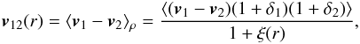 (1)where v and
δ are the
peculiar velocity and density contrast, respectively, and ξ is the two-point
correlation function. Since the line-of-sight velocities of discrete galaxies are measured
for each sample, Ferreira et al. (1999) proposed that
the estimator of the pairwise velocity is
(1)where v and
δ are the
peculiar velocity and density contrast, respectively, and ξ is the two-point
correlation function. Since the line-of-sight velocities of discrete galaxies are measured
for each sample, Ferreira et al. (1999) proposed that
the estimator of the pairwise velocity is ![Mathematical equation: \begin{eqnarray} v_{12}(r)=\left[2 \sum (s_{\rm A}-s_{\rm B})p_{\rm AB}\right] \Big/ \left[\sum p^{2}_{\rm AB}\right], \label{eq:pairwise-estimate} \end{eqnarray}](/articles/aa/full_html/2015/11/aa26051-15/aa26051-15-eq15.png) (2)where
(2)where  is the line-of-sight velocity of galaxy A,
 is the geometric factor, and the summation
is for all pairs within a distance separation bin Δr. It was first proposed in Ferreira et al. (1999) that the estimator measures the cosmological
density parameter Ω, and later
it was found in Juszkiewicz et al. (2000) that the
matter density of the Universe is close to 0.35 and that the Einstein-de Sitter model Ω = 1 is inconsistent with the data. The
result of a low-density universe was further confirmed by Feldman et al. (2003) with the Mark III catalogue, Spiral Field I-Band (SFI) catalogue,
Nearby Early-type Galaxies Survey (ENEAR) catalogue, and the Revised Flat Galaxy Catalog
(RFGC). This becomes the early measurement of matter content of the Universe before the
experiment of the cosmic microwave background radiation from Wilkinson
Microwave Anisotropy Probe (WMAP) and strongly indicates that there is
Λ in the cosmic budget. In
addition, Juszkiewicz et al. (1999) investigated the
dynamics of the pairwise motion by calibrating the mean pairwise velocity with
N-body
simulations. They provide a theoretical formula that is very consistent with the
N-body
simulation result. Additionally, Bhattacharya & Kosowsky
(2007) forecast the prospective constraints on cosmological parameters from the
pairwise kinetic Sunyaev-Zeldovich effect (proportional to velocity field). In 2012, by
applying the pairwise momentum estimator of Ferreira et al.
(1999) into the temperature map, the Atacama Cosmology Telescope team (ACT)
provided the first detection of the kinetic Sunyaev-Zeldovich effect (Hand et al. 2012). More recently, Planck
Collaboration Int. XXXVII (2015) have estimated the pairwise momentum of the kSZ
temperature fluctuations of Planck maps at the positions of the Central
Galaxy Catalogue samples extracted from Sloan Digital Sky Survey (SDSS-DR7) data. They find
a ~2σ CL detection of the kSZ
signal, which is consistent and slightly lower than the one found in Hand et al. (2012).
is the geometric factor, and the summation
is for all pairs within a distance separation bin Δr. It was first proposed in Ferreira et al. (1999) that the estimator measures the cosmological
density parameter Ω, and later
it was found in Juszkiewicz et al. (2000) that the
matter density of the Universe is close to 0.35 and that the Einstein-de Sitter model Ω = 1 is inconsistent with the data. The
result of a low-density universe was further confirmed by Feldman et al. (2003) with the Mark III catalogue, Spiral Field I-Band (SFI) catalogue,
Nearby Early-type Galaxies Survey (ENEAR) catalogue, and the Revised Flat Galaxy Catalog
(RFGC). This becomes the early measurement of matter content of the Universe before the
experiment of the cosmic microwave background radiation from Wilkinson
Microwave Anisotropy Probe (WMAP) and strongly indicates that there is
Λ in the cosmic budget. In
addition, Juszkiewicz et al. (1999) investigated the
dynamics of the pairwise motion by calibrating the mean pairwise velocity with
N-body
simulations. They provide a theoretical formula that is very consistent with the
N-body
simulation result. Additionally, Bhattacharya & Kosowsky
(2007) forecast the prospective constraints on cosmological parameters from the
pairwise kinetic Sunyaev-Zeldovich effect (proportional to velocity field). In 2012, by
applying the pairwise momentum estimator of Ferreira et al.
(1999) into the temperature map, the Atacama Cosmology Telescope team (ACT)
provided the first detection of the kinetic Sunyaev-Zeldovich effect (Hand et al. 2012). More recently, Planck
Collaboration Int. XXXVII (2015) have estimated the pairwise momentum of the kSZ
temperature fluctuations of Planck maps at the positions of the Central
Galaxy Catalogue samples extracted from Sloan Digital Sky Survey (SDSS-DR7) data. They find
a ~2σ CL detection of the kSZ
signal, which is consistent and slightly lower than the one found in Hand et al. (2012).
The literature listed above about the pairwise velocity estimator is for the old data set, whereas this work uses a new data set, the new compiled Cosmicflows-2 catalogue, to constrain cosmology. In addition, we developed a new method of computing the covariance matrix of the pairwise velocity field and formed a likelihood that directly relates the models of pairwise velocity field with the data. The paper is organized as follows. In Sect. 2, we introduce the new Cosmicflows-2 data set. In Sect. 3, we introduce our statistical method of computing the likelihood of pairwise velocities. In Sect. 4, we present our results of constraints and compare them with WMAP nine-year cosmology and Planck 2015 cosmology. The conclusion is presented in the last section.
Throughout the paper, unless otherwise stated, we use Planck 2015 best-fitting cosmological parameters (Planck Collaboration XIII 2015), i.e. {Ωm, σ8, h, Ωb, ln(1010As)}={0.309, 0.816, 0.677, 0.049, 3.064}.
2. Data set
The Cosmicflows-2 catalogue (Tully et al. 2013) is a compiled catalogue of distances and peculiar velocities of more than 8000 galaxy samples. Some of these samples are from new measurements, while others are taken from the literature. The majority of the distances of the samples are measured through the Tully-Fisher relation (Tully & Fisher 1977) or fundamental-plane (FP) relation (Djorgovski & Davis 1987; Campbell et al. 2014) with roughly 20 per cent of the error for the distances. But there are a small portion of the samples whose distances are measured from Type-Ia supernovae light curves, surface brightness fluctuation, the tip of the red giant branch (TRGB), or Cepheids. The Cosmicflows-2 samples are calibrated at their zero points by using two different approaches. One is to use the Cepheid period-luminosity relation (Cepheid PLR), and the other to use the luminosities of red giant branch stars at the onset of core helium burning, at a location in a stellar colour–magnitude diagram (CMD) known as the TRGB.
Eventually, the correlation between the galaxy luminosity and HI line width was refitted so zero points were determined (Tully et al. 2013). In addition, Tully & Courtois (2012) have demonstrated that no extra systematics were found after the zero-point calibration. The results of the two methods of re-calibrations were compared, which confirmed that the distance estimation is unbiased (Tully et al. 2013). We obtained these samples from the “VizieR” astronomy data base, which are available in two tables. Table I provides the entry for every galaxy with a distance, consisting of 8315 galaxies in total. Table II condenses the galaxies in each group and provides a distance for each group, therefore consisting 5224 group entries. In the following analysis, we use both tables in the pairwise velocity analysis, so we name Table I as GALAXY and Table II as GROUP in the following text.
We made one adjustment of the observed peculiar velocities in the Cosmicflows-2 samples.
On page 20 of Tully et al. (2013), it is stated that
the line-of-sight peculiar velocity is calculated through cz −
H0d, where d is the measured distance.
However, as shown in Davis & Scrimgeour (2014) and
Watkins & Feldman (2015a), this estimator makes
the velocity estimate biased at the level Δvp ~ 100 km s-1 at
z ~ 0.04 and
even more biased at higher redshifts. The more accurate formula for calculating the
line-of-sight velocity is (Davis & Scrimgeour
2014) 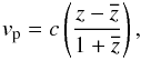 (3)where z is the measured redshift,
and
(3)where z is the measured redshift,
and  is the redshift for the unperturbed
background. One can obtain by inverting the measured luminosity
distance
is the redshift for the unperturbed
background. One can obtain by inverting the measured luminosity
distance 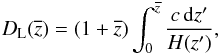 (4)where
 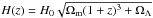 is the Hubble parameter. In Fig. 1, we show the measured velocity difference of
GROUP catalogue between Eq. (3) and the Col. 20 of Table II in Tully
et al. (2013). One can see that by adjusting the peculiar velocity calculation,
there is a trend towards lower velocity values, which indicates that the original velocities
provided by Tully et al. (2013) are biased towards
higher velocity values. This is consistent with the prediction shown in Figs. 2 and 3 in Davis &
Scrimgeour (2014)1. In addition, we propagate
the distance error into the peculiar velocities and plot the histogram of the rms velocity
errors in the upper panel of Fig. 2. One can see that
the two histograms peak at slightly different values, i.e. 500–1000 and 1000 km s-1, respectively. We use
the propagated velocity errors as the measurement error in the likelihood analysis.
is the Hubble parameter. In Fig. 1, we show the measured velocity difference of
GROUP catalogue between Eq. (3) and the Col. 20 of Table II in Tully
et al. (2013). One can see that by adjusting the peculiar velocity calculation,
there is a trend towards lower velocity values, which indicates that the original velocities
provided by Tully et al. (2013) are biased towards
higher velocity values. This is consistent with the prediction shown in Figs. 2 and 3 in Davis &
Scrimgeour (2014)1. In addition, we propagate
the distance error into the peculiar velocities and plot the histogram of the rms velocity
errors in the upper panel of Fig. 2. One can see that
the two histograms peak at slightly different values, i.e. 500–1000 and 1000 km s-1, respectively. We use
the propagated velocity errors as the measurement error in the likelihood analysis.
We plot the redshift distribution of GALAXY and GROUP catalogues in the lower panel of Fig. 2. One can see that the bulk of the samples are in the range of 0–15 000 km s-1, while a few samples reside at higher redshifts. The two catalogues are probing the same redshift range. The GROUP catalogue is just a scaled-down version of the GALAXY catalogue, since GROUP is just a condensation of the GALAXY catalogue. In Fig. 3, we plot the re-adjusted peculiar velocities (through Eq. (3)) of two catalogues on the sky in the Galactic coordinate, so the Galactic plane region is empty. The red (light grey) points are moving away from us, and the blue (dark grey) points are moving towards us. The size of the points is proportional to the magnitude of the line-of-sight peculiar velocity. One can see that the velocity distribution is almost uniform across the full sky.
3. Methodology
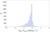 |
Fig. 1 Histogram of the line-of-sight peculiar velocity difference in the GROUP catalogue between the calculation by using Eq. (3) (labelled as VMa) and the values given in Tully et al. (2013) (labelled as VTully). |
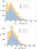 |
Fig. 2 Top: histogram of the measured velocity error of GALAXT (Orange) and GROUP (blue) catalogues. The two histograms peak at 500–1000 and 1000 km s-1, respectively. The bin width of the histogram is Δσ(vp) = 200 km s-1. Bottom: histogram of redshift distribution of GALAXY and GROUP samples. The bin width of the plot is cΔz = 2000 km s-1. |
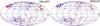 |
Fig. 3 Full-sky GALAXY (8315 samples) and GROUP (5224 samples) catalogues plotted in Galactic coordinates. The red (light grey) points are moving away from us, and the blue (dark grey) points towards us. The size of the points is proportional to the magnitude of the line-of-sight peculiar velocity. |
In this section, we first present three theoretical models of pairwise velocity field, and then discuss how can we simulate the covariance matrix of the pairwise velocity estimator at different distance bins. Then we present the likelihood function.
3.1. Theoretical models
Equation (1) is the definition of pairwise
velocity field at each separate distance r. The approximate solution of the pairwise
velocity field through the pair conservation equation derived by Juszkiewicz et al. (1999) is given as (also see Feldman et al. 2003) ![Mathematical equation: \begin{eqnarray} v_{12}(r) & = & -\frac{2}{3}\Omega^{0.6}_{\rm m} H_{0} r \bar{\xi}(r)(1+\alpha \bar{\xi}(r)), \\ \label{eq:v12-r-theory} \hspace*{-4mm}\bar{\xi}(r) & = & \left[3 \int^{r}_{0}\xi(x)x^{2}\der x\right] \Big/ \left[r^{3}(1+\xi(r))\right] ,\label{eq:xi-r} \end{eqnarray}](/articles/aa/full_html/2015/11/aa26051-15/aa26051-15-eq44.png) where α = 1.2−0.65γ, and γ = −(dlnξ/dlnr) | ξ = 1.
ξ(r) can be measured directly from
galaxy surveys two-point correlation statistics. Here we use the two-point correlation
function of Point Source Catalogue redshift survey (PSCz) calculated by Hamilton & Tegmark (2002). This is because the
PSCz survey
measures the galaxy distance out to 120
h-1 Mpc and its sky coverage is close to
the Cosmicflows-2 catalogue (see panels a, b, and d of Fig. 1 in Ma et al. 2012). Thus the PSCz covers the similar volume of the local Universe
as Cosmicflows-2 . The ξ(r) model derived by
PSCz survey
(Hamilton & Tegmark 2002) is
where α = 1.2−0.65γ, and γ = −(dlnξ/dlnr) | ξ = 1.
ξ(r) can be measured directly from
galaxy surveys two-point correlation statistics. Here we use the two-point correlation
function of Point Source Catalogue redshift survey (PSCz) calculated by Hamilton & Tegmark (2002). This is because the
PSCz survey
measures the galaxy distance out to 120
h-1 Mpc and its sky coverage is close to
the Cosmicflows-2 catalogue (see panels a, b, and d of Fig. 1 in Ma et al. 2012). Thus the PSCz covers the similar volume of the local Universe
as Cosmicflows-2 . The ξ(r) model derived by
PSCz survey
(Hamilton & Tegmark 2002) is ![Mathematical equation: \begin{eqnarray} \xi(r)=\left(\frac{\sigma_{8}}{0.83} \right)^{2}\left[\left(\frac{r}{r_{1}} \right)^{-\gamma_{1}} + \left(\frac{r}{r_{2}} \right)^{-\gamma_{2}} \right], \label{eq:model1} \end{eqnarray}](/articles/aa/full_html/2015/11/aa26051-15/aa26051-15-eq49.png) (7)where r1 = 2.33
h-1 Mpc, r2 = 3.51
h-1 Mpc, γ1 = 1.72,
γ2 =
1.28, and σ8 is a free parameter.
(7)where r1 = 2.33
h-1 Mpc, r2 = 3.51
h-1 Mpc, γ1 = 1.72,
γ2 =
1.28, and σ8 is a free parameter.
We name the above PSCz model as Model 1 in the following discussion. In
addition, we also consider two other simplified models of the correlation function as
(Feldman et al. 2003) 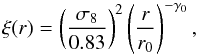 (8)where (γ0,
r0) = (1.3, 4.76 h-1 Mpc)
and (1.8, 4.6 h-1 Mpc) for
Models 2 and 3, respectively.
(8)where (γ0,
r0) = (1.3, 4.76 h-1 Mpc)
and (1.8, 4.6 h-1 Mpc) for
Models 2 and 3, respectively.
We vary two parameters in the pairwise velocity field model. One is σ8, which is the
square root of the amplitude of the two-point correlation function (Eqs. (7) and (8)). But because ξ(r) affects both the numerator
and denominator of  (Eq. (6)), σ8 will affect
the shape of the pairwise velocity field function v12(r). In addition, we
also vary the total amplitude parameter
(Eq. (6)), σ8 will affect
the shape of the pairwise velocity field function v12(r). In addition, we
also vary the total amplitude parameter  as the pre-factor in Eq. (6).
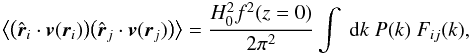
The three model predictions plotted in Fig. 5 are all negative in the regime of 0–30 Mpc, because of the gravitational potential effect. In addition, one can see that Models 1 and 2 predictions are close to each other, while Model 3 has slightly lower power on a large separation r ~ 30 Mpc.
3.2. Covariance matrix
We now calculate the covariance matrix for the pairwise velocity estimator. In the original work of Ferreira et al. (1999), the covariance matrix is calculated analytically by assuming a smoothed survey window function. However, this is only an approximation since the real survey window can have complicated geometry. Here we calculate the covariance matrix of pairwise velocity field directly from a numerical simulation that automatically includes the real survey geometry.
We simulated a large number of mock catalogues. For each simulation, we simulated Ndata = 8315 and 5224 samples’ line-of-sight velocities for GALAXY and GROUP catalogues and then computed the pairwise velocities from Eq. (1). Then we calculated the variance of the pairwise velocity field from these mock catalogues. We tested that Nsim = 103 is large enough for the results to converge.
3.2.1. Covariance matrix of line-of-sight velocities
As one can see from Eqs. (14)–(16) of Ma & Scott
(2013), the line-of-sight velocities are correlated. We therefore need to
calculate the covariance matrix of these line-of-sight velocities before simulation. For
any two samples, their covariance matrix is 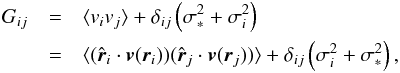 (9)where the first term is the cosmic variance
term since the intrinsic correlation between velocities at two different directions. The
second bracket contains the rms measurement noise for each galaxy
σi (i.e. quantity
plotted in the upper panel of Fig. 2) and the small
scale and intrinsic dispersion σ∗ which is estimated to be around
200 km s-1
(Turnbull et al. 2012).
(9)where the first term is the cosmic variance
term since the intrinsic correlation between velocities at two different directions. The
second bracket contains the rms measurement noise for each galaxy
σi (i.e. quantity
plotted in the upper panel of Fig. 2) and the small
scale and intrinsic dispersion σ∗ which is estimated to be around
200 km s-1
(Turnbull et al. 2012).
For the cosmic variance term, any two samples are correlated so the off-diagonal
element of Gij
(i ≠
j) is non-zero. But for the measurement noise term,
small scale, and intrinsic dispersion, the two samples are not correlated, so they only
contribute to the diagonal term in the Gij matrix. The first
term is the real space velocity correlation function, which is related to the matter
power spectrum in Fourier space (Watkins et al.
2009; Ma & Scott 2013),
 (10)where P(k) is
the matter power spectrum that we output from public code camb (Lewis et al. 2000). The f(z) =
dlnD/ dlna is
the growth rate function that characterizes how fast the structures grow at different
epochs of the Universe. Since the Cosmicflows-2 samples peak at the redshift
z ≃
0.0167 (lower panel of Fig. 2),
we use the zero-redshift growth function
(10)where P(k) is
the matter power spectrum that we output from public code camb (Lewis et al. 2000). The f(z) =
dlnD/ dlna is
the growth rate function that characterizes how fast the structures grow at different
epochs of the Universe. Since the Cosmicflows-2 samples peak at the redshift
z ≃
0.0167 (lower panel of Fig. 2),
we use the zero-redshift growth function  (Watkins
et al. 2009; Ma & Scott 2013) in Eq.
(10). In the future, if the survey
probes deeper region of the space, one should use the corresponding growth function
f(z) in Eq. (10), so that the joint constraints on
f(z)σ8
can be obtained, which constitutes a sensitive test of modify gravity models (Hudson & Turnbull 2012; Planck Collaboration XIII 2015).
(Watkins
et al. 2009; Ma & Scott 2013) in Eq.
(10). In the future, if the survey
probes deeper region of the space, one should use the corresponding growth function
f(z) in Eq. (10), so that the joint constraints on
f(z)σ8
can be obtained, which constitutes a sensitive test of modify gravity models (Hudson & Turnbull 2012; Planck Collaboration XIII 2015).
The Fij(k)
is the window function 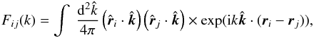 (11)which can be calculated analytically
(Appendix in Ma et al. 2011).
(11)which can be calculated analytically
(Appendix in Ma et al. 2011).
Therefore, by calculating Gij matrix, we obtain a Ndata × Ndata covariance matrix for the line-of-sight velocities of mock galaxies. We then followed the procedure in Appendix A to simulate a mock line-of-sight velocity catalogue. We did this repeatedly for Nsim number of mock catalogues.
3.2.2. Covariance matrix for pairwise velocities
For each mock catalogue, we can plug them into Eq. (2) to obtain v12(r) for different
bins, then one can obtain Nsim numbers of mock v12 velocity
fields. Then, for each distance bin, one can calculate the covariance matrix for
Nbin as  (12)Therefore, this Cij is a
Nbin ×
Nbin positive-definite symmetric matrix
which is the covariance matrix for v12(r).
(12)Therefore, this Cij is a
Nbin ×
Nbin positive-definite symmetric matrix
which is the covariance matrix for v12(r).
In Fig. 4, we plot the covariance matrix of the GALAXY catalogue. One can see that it is a positive and symmetric matrix, and the higher value of correlation exists on large separation distances. This is because the cosmic variance term becomes more significant at a larger separation distance. In Fig. 5, we plot the square root of the diagonal value of covariance matrix as the error bars for GALAXY and the GROUP catalogue as an example for Nbin = 14. But here we remind the reader that the correlation between different data points is significant, so the value of the square-root cannot fully represent the total error budget.
3.3. Likelihood
We now have the models, measured peculiar velocity field data, and the covariance matrix
ready. Our purpose is to fit the amplitude of matter fluctuation parameter σ8 and the
combined parameter  with the pairwise velocity data. We
formulate a log-likelihood function as
with the pairwise velocity data. We
formulate a log-likelihood function as 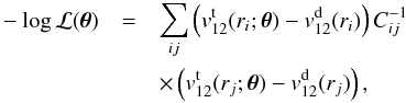 (13)where the indexes “t” and “d” mean “theory”
and “data” respectively, and θ represents the parameters of
interest. Maximizing this likelihood function will give us the estimate of the
cosmological parameter θ.
(13)where the indexes “t” and “d” mean “theory”
and “data” respectively, and θ represents the parameters of
interest. Maximizing this likelihood function will give us the estimate of the
cosmological parameter θ.
4. Results
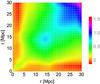 |
Fig. 4 Covariance matrix of v12(r) for GALAXY catalogue. The x- and y-axis mean the different radial bins, and the unit of colour bar is 100 km s-1. |
 |
Fig. 5 v12(r) for the GALAXY and GROUP catalogues with the data points calculated from Eq. (2) and error bars from the square root of Eq. (12). The black, red dashed, and blue dashed lines are for Models 1, 2, and 3, respectively, by using Planck 2015 best-fitting cosmological parameters. The measured v12(r) is separated into 14 bins, and the error bars between each bin are highly correlated. |
 |
Fig. 6 Joint constraints on |
In Fig. 5, the three models are plotted with Planck 2015 best-fitting cosmological parameters, which seems to be consistent with both GALAXY and GROUP data sets. However, the error bars in Fig. 5 are highly correlated (Fig. 4), so we need to use the full covariance matrix to derive more quantitative results.
We now present our final results for the likelihood analysis. In Fig. 6, we plot the joint constraints on
and σ8 from
GALAXY and GROUP catalogues, for three
theoretical models. The black-diamond and orange-square marks are the best-fitting
parameters from the WMAP nine-year results and Planck 2015 results. One can
see that the joint constraints from the GALAXY catalogue (upper
panels) contain the best-fitting point of the cosmic microwave background (CMB) survey at
around 1σ CL,
which indicates that they are highly consistent with the ΛCDM model with WMAP or Planck
cosmological parameters. For the GROUP catalogue (lower
panels), although the best-fitting parameter values from CMB are not within the
1σ CL of the
joint constraints, they are consistent with pairwise velocity constraints at 2σ CL, which is not big
enough to claim any discrepancy.
Comparing the six panels, we conclude that the current tightest constraint on cosmological
parameters is from the GROUP catalogue with parameter values as
 (14)Looking into the future, the potential for
enhancing the constraining power of the pairwise velocity field is embodied in the following
aspects.
(14)Looking into the future, the potential for
enhancing the constraining power of the pairwise velocity field is embodied in the following
aspects.
-
1.
Better modelling of the pairwise velocity from simulations ofthe large-scale structure. By developing a numerical simulation,Slosar et al. (2006) investigatedthe distribution of velocities of pairs at a given separation tak-ing both one-halo and two-halo contributions into account.Later on, Lam et al. (2011)studied how primordial non-Gaussianity affects the pairwisevelocity probability density function by using an analyticalmodel and the N-body simulations. More recently, Thompson &Nagamine (2012) have investigated the velocitydistribution of dark matter halo pairs in large N-body simulations(250 h-1 Mpc–1 h-1 Gpc) and examined the pairwise halo velocities with high velocity bullet cluster samples. These efforts at more accurate modelling of pairwise velocity field will continue and lead to the closer description of the observed pairwise velocity data.
-
2.
Better calibration of the distance estimate and the reduction of distance error. The most important aspect of enhancing cosmological constraints on a pairwise velocity field is to improve the distance estimate. Currently, the Tully-Fisher (Tully & Fisher 1977) and FP (Djorgovski & Davis 1987; Campbell et al. 2014) relations lead to the distance estimate in the range of 25–30 per cent. For instance, for the FP distance estimator, the total scattering of distance r constitutes intrinsic scatters (~20 per cent), FP slope multiplied the observational error (~18 per cent) and the photometric error (~3 per cent). The bulk part, i.e. intrinsic scatters, is due in part to the effect of stellar population age variations on M/L, but the very large uncertainties on individual age estimates mean that it is very difficult to correct the effect (Campbell et al. 2014). Therefore, much effort needs to be devoted to investigating those effects that strongly affect intrinsic scattering.
-
3.
Denser and broader sky coverage. These two factors in total will lead to providing more samples for each individual distance bin so that the rms noise level will be reduced as the sample size increases. In addition, since the Tully-Fisher survey needs to measure the HI line width, they are limited by the flux of HI measurement (Masters et al. 2006; Catinella et al. 2007). The Fundamental Plane survey measures the galaxy’s surface brightness, so it is limited by the sensitivity of the telescope (telescope size, exposure time, atmospheric interference, etc.). For these reasons, the faint galaxies are hard to measure, and the density in the survey volume is limited. As a rough estimate of the current state-of-the-art 6dF galaxy survey, the sampling density at z1 / 2 ≃ 0.05 is ρ = 4 × 10⁻³h3 Mpc-3 (Campbell et al. 2014).
-
4.
Deeper redshift and distance surveys. The survey volume is an important factor in improving the dark energy and modified gravity constraints. This is not only because the deeper survey provides more samples, but also because it provides estimates of the growth of the structure at different redshifts. As a result, for a much deeper survey, one can separate the pairwise velocity samples into different redshift bins and constrain the f(z)σ8 value in Eq. (10). The redshift evolution of f(z)σ8 in the regime of z = 0–1 constitutes a sensitive probe of the modified gravity and dark energy, which has been demonstrated in Hudson & Turnbull (2012) and Planck Collaboration XIII (2015).
-
5.
Alternative velocity probe of the kinetic Sunyaev-Zeldovich effect (Sunyaev & Zeldovich 1972, 1980). The kinetic Sunyaev-Zeldovich effect (kSZ) is the secondary anisotropy of the CMB produced by the inverse Compton scattering of the moving electrons. The temperature anisotropy of the CMB is therefore proportional to the line-of-sight peculiar velocities of the electrons, i.e.
 . Thus, the accurate measurement of the
kSZ effect from CMB observations and the precise modelling of intergalactic gas can,
in principle, lead to determining the pairwise velocity field without suffering from
systematics from optical survey. The pairwise momentum of the temperature field in
Hand et al. (2012) gave the first detection
of the kSZ effect by using the ACT data. More recently, Planck Collaboration Int. XXXVII (2015) have re-measured the
pairwise momentum field by using Planck 2015 data and
cross-correlated the temperature field with the reconstructed peculiar velocity field.
For the first time, they find the 3–3.7σ CL detection of this correlation, which
indicates that the gas is extended much beyond the virial radii of dark matter halo,
constituting direct evidence of the low-density, diffuse baryons (Planck Collaboration Int. XXXVII 2015; Hernández-Monteagudo et al. 2015). The effort of
accurately measuring kSZ effect will carry on and will improve the peculiar velocity
field measurement from the channel different from optical surveys.
. Thus, the accurate measurement of the
kSZ effect from CMB observations and the precise modelling of intergalactic gas can,
in principle, lead to determining the pairwise velocity field without suffering from
systematics from optical survey. The pairwise momentum of the temperature field in
Hand et al. (2012) gave the first detection
of the kSZ effect by using the ACT data. More recently, Planck Collaboration Int. XXXVII (2015) have re-measured the
pairwise momentum field by using Planck 2015 data and
cross-correlated the temperature field with the reconstructed peculiar velocity field.
For the first time, they find the 3–3.7σ CL detection of this correlation, which
indicates that the gas is extended much beyond the virial radii of dark matter halo,
constituting direct evidence of the low-density, diffuse baryons (Planck Collaboration Int. XXXVII 2015; Hernández-Monteagudo et al. 2015). The effort of
accurately measuring kSZ effect will carry on and will improve the peculiar velocity
field measurement from the channel different from optical surveys.
5. Conclusion
In this work, we have developed a Bayesian statistics method for using a galaxy pairwise velocity field to estimate cosmological parameters. We first reviewed the pairwise velocity estimator developed in Ferreira et al. (1999) to calculate the relative motion between galaxy pairs with a separation distance between 0 and 30 h-1 Mpc, and then we review three theoretical models of the mean pairwise velocity field, especially the one used in Juszkiewicz et al. (1999), which was calibrated against N-body simulation.
We then focused our effort on simulating mock galaxy catalogues and calculated the
log-likelihood function of the pairwise velocity field. We first calculated the covariance
matrix between any two line-of-sight velocities in a given survey and simulated the
103 mock catalogue
according to this covariance matrix. Then we calculated the pairwise velocity field for each
of these mock catalogues and calculated the variance of the v12(r). In this way, we
obtained a covariance matrix of the v12(r) field and used
this in the likelihood to estimate cosmological parameters
and σ8. By using the
Cosmicflows-2 catalogue, which consists of over 8000 galaxies over the full sky out to
25 000 km s-1, we
show that the results are consistent with the WMAP nine-year data and
Planck 2015 data, and the error bars are currently too big to draw any
concrete conclusion on modified gravity models or dynamical dark energy2. We hope therefore that future data with more samples on the local
Universe may help to pin down the sample variance and improve pairwise velocity field
statistics.
The re-adjusted peculiar velocities of Cosmicflows-2 catalogue can be requested from the corresponding author.
In this sense, we think what is claimed in Hellwing et al. (2014) is too optimistic.
Acknowledgments
We would like to thank Chris Blake, Helene Courtois, Elisabete da Cunha, Tamara Davis, Hume Feldman, Pedro Ferreira, Andrew Johnson, and Jeremy Mould for helpful discussions. We also acknowledge the use of the “VizieR” astronomy online database and camb package. Y.Z.M. acknowledges support from an ERC Starting Grant (No. 307209), and P.H. acknowledges support by the National Science Foundation of China (No. 11273013) and by the Open Project Program of State Key Laboratory of Theoretical Physics, Institute of Theoretical Physics, Chinese Academy of Sciences, China (No. Y4KF121CJ1).
References
- Bhattacharya, S., &Kosowsky, A. 2007, ApJ, 659, L83 [NASA ADS] [CrossRef] [Google Scholar]
- Branchini, E., Zehavi, I., Plionis, M., &Dekel, A. 2000, MNRAS, 313, 491 [NASA ADS] [CrossRef] [Google Scholar]
- Branchini, E., Freudling, W., Da Costa, L. N., et al. 2001, MNRAS, 326, 1191 [NASA ADS] [CrossRef] [Google Scholar]
- Campbell, L. A., Lucey, J. R.,Colless, M., et al. 2014, MNRAS, 443, 1231 [NASA ADS] [CrossRef] [Google Scholar]
- Catinella, B., Haynes, M. P., &Giovanelli, R. 2007, AJ, 134, 334 [NASA ADS] [CrossRef] [Google Scholar]
- Davis, T. M., &Scrimgeour, M. I. 2014, MNRAS, 442, 1117 [NASA ADS] [CrossRef] [Google Scholar]
- Davis, M., Nusser, A., Masters, K. L., et al. 2011, MNRAS, 413, 2906 [NASA ADS] [CrossRef] [Google Scholar]
- Dekel, A., Bertschinger, E., Yahil, A., et al. 1993, ApJ, 412, 1 [NASA ADS] [CrossRef] [Google Scholar]
- Dekel, A., Eldar, A., Kolatt, T., et al. 1999, ApJ, 522, 1 [NASA ADS] [CrossRef] [Google Scholar]
- Djorgovski, S., &Davis, M. 1987, ApJ, 313, 59 [NASA ADS] [CrossRef] [Google Scholar]
- Feldman, H., Juszkiewicz, R., Ferreira, P., et al. 2003, ApJ, 596, L131 [NASA ADS] [CrossRef] [Google Scholar]
- Feldman, H. A.,Watkins, R., & Hudson, M. J. 2010, MNRAS, 407, 2328 [NASA ADS] [CrossRef] [Google Scholar]
- Ferreira, P. G.,Juszkiewicz, R., Feldman, H. A., Davis, M., &Jaffe, A. H. 1999, ApJ, 515, L1 [NASA ADS] [CrossRef] [Google Scholar]
- Hamilton, A. J. S., &Tegmark, M. 2002, MNRAS, 330, 506 [NASA ADS] [CrossRef] [Google Scholar]
- Hand, N., Addison, G. E.,Aubourg, E., et al. 2012, Phys. Rev. Lett., 109, 041101 [NASA ADS] [CrossRef] [Google Scholar]
- Hellwing, W. A.,Barreira, A.,Frenk, C. S.,Li, B., &Cole, S. 2014, Phys. Rev. Lett., 112, 221102 [NASA ADS] [CrossRef] [Google Scholar]
- Hernández-Monteagudo, C., Ma, Y.-Z., Kitaura, F.-S., et al. 2015, Arxiv e-prints [arXiv:1504.04011] [Google Scholar]
- Hinshaw, G., Larson, D., Komatsu, E., et al. 2013, ApJS, 208, 19 [NASA ADS] [CrossRef] [Google Scholar]
- Hudson, M. J., &Turnbull, S. J. 2012, ApJ, 751, L30 [NASA ADS] [CrossRef] [Google Scholar]
- Hudson, M. J., Dekel, A., Courteau, S., Faber, S. M., &Willick, J. A. 1995, MNRAS, 274, 305 [NASA ADS] [CrossRef] [Google Scholar]
- Johnson, A., Blake, C., Koda, J., et al. 2014, MNRAS, 444, 3926 [NASA ADS] [CrossRef] [Google Scholar]
- Juszkiewicz, R., Fisher, K. B., &Szapudi, I. 1998, ApJ, 504, L1 [NASA ADS] [CrossRef] [Google Scholar]
- Juszkiewicz, R., Springel, V., &Durrer, R. 1999, ApJ, 518, L25 [NASA ADS] [CrossRef] [Google Scholar]
- Juszkiewicz, R., Ferreira, P. G.,Feldman, H. A.,Jaffe, A. H., & Davis, M. 2000, Science, 287, 109 [NASA ADS] [CrossRef] [Google Scholar]
- Kashlinsky, A., Atrio-Barandela, F., Kocevski, D., &Ebeling, H. 2008, ApJ, 686, L49 [NASA ADS] [CrossRef] [Google Scholar]
- Lam, T. Y.,Nishimichi, T., & Yoshida, N. 2011, MNRAS, 414, 289 [NASA ADS] [CrossRef] [Google Scholar]
- Lewis, A., Challinor, A., &Lasenby, A. 2000, ApJ, 538, 473 [NASA ADS] [CrossRef] [Google Scholar]
- Ma, Y.-Z., &Scott, D. 2013, MNRAS, 428, 2017 [NASA ADS] [CrossRef] [Google Scholar]
- Ma, Y.-Z., Gordon, C., &Feldman, H. A. 2011, Phys. Rev. D, 83, 103002 [NASA ADS] [CrossRef] [Google Scholar]
- Ma, Y.-Z., Branchini, E., &Scott, D. 2012, MNRAS, 425, 2880 [NASA ADS] [CrossRef] [Google Scholar]
- Macaulay, E., Feldman, H., Ferreira, P. G., Hudson, M. J., &Watkins, R. 2011, MNRAS, 414, 621 [NASA ADS] [CrossRef] [Google Scholar]
- Macaulay, E., Feldman, H. A.,Ferreira, P. G., et al. 2012, MNRAS, 425, 1709 [NASA ADS] [CrossRef] [Google Scholar]
- Masters, K. L.,Springob, C. M., Haynes, M. P., & Giovanelli, R. 2006, ApJ, 653, 861 [NASA ADS] [CrossRef] [Google Scholar]
- Nusser, A., &Davis, M. 2011, ApJ, 736, 93 [NASA ADS] [CrossRef] [Google Scholar]
- Peebles, P. J. E. 1993, Principles of Physical Cosmology, ed. P. J. E. Peebles (Princeton University Press) [Google Scholar]
- Pike, R. W., &Hudson, M. J. 2005, ApJ, 635, 11 [NASA ADS] [CrossRef] [Google Scholar]
- Planck Collaboration XVI. 2014, A&A, 571, A16 [NASA ADS] [CrossRef] [EDP Sciences] [Google Scholar]
- Planck Collaboration XIII. 2015, A&A, submitted [arXiv:1502.01589] [Google Scholar]
- Planck Collaboration Int. XXXVII. 2015, A&A, accepted, [arXiv:1504.03339] [Google Scholar]
- Sigad, Y., Eldar, A., Dekel, A., Strauss, M. A., &Yahil, A. 1998, ApJ, 495, 516 [NASA ADS] [CrossRef] [Google Scholar]
- Slosar, A., Seljak, U., &Tasitsiomi, A. 2006, MNRAS, 366, 1455 [NASA ADS] [CrossRef] [Google Scholar]
- Sunyaev, R. A., &Zeldovich, Y. B. 1972, Comm. Astrophys. Space Phys., 4, 173 [Google Scholar]
- Sunyaev, R. A., &Zeldovich, I. B. 1980, MNRAS, 190, 413 [NASA ADS] [CrossRef] [Google Scholar]
- Thompson, R., &Nagamine, K. 2012, MNRAS, 419, 3560 [NASA ADS] [CrossRef] [Google Scholar]
- Tully, R. B., &Courtois, H. M. 2012, ApJ, 749, 78 [NASA ADS] [CrossRef] [Google Scholar]
- Tully, R. B., &Fisher, J. R. 1977, A&A, 54, 661 [NASA ADS] [Google Scholar]
- Tully, R. B.,Courtois, H. M., Dolphin, A. E., et al. 2013, AJ, 146, 86 [NASA ADS] [CrossRef] [Google Scholar]
- Turnbull, S. J., Hudson, M. J.,Feldman, H. A., et al. 2012, MNRAS, 420, 447 [NASA ADS] [CrossRef] [Google Scholar]
- Watkins, R., &Feldman, H. A. 2015a, MNRAS, 450, 1868 [NASA ADS] [CrossRef] [Google Scholar]
- Watkins, R., &Feldman, H. A. 2015b, MNRAS, 447, 132 [NASA ADS] [CrossRef] [Google Scholar]
- Watkins, R., Feldman, H. A., &Hudson, M. J. 2009, MNRAS, 392, 743 [NASA ADS] [CrossRef] [Google Scholar]
Appendix A: Simulating a catalogue given its covariance matrix
The Gij is a symmetric,
positive-definite matrix, where we can use the singular value decomposition (SVD) method
to simulate the velocity vector vi (i =
1,...,Ndata).
The G matrix can be decomposed into  (A.1)where U is the left matrix, and
its transpose is the right matrix, and the S matrix is the diagonal matrix
with Ndata element that contains the
eigenvalues of matrix G. Since G is a positive-definite matrix,
the elements in S should be positive. Then we can simulate an array
of Gaussian random variables
(A.1)where U is the left matrix, and
its transpose is the right matrix, and the S matrix is the diagonal matrix
with Ndata element that contains the
eigenvalues of matrix G. Since G is a positive-definite matrix,
the elements in S should be positive. Then we can simulate an array
of Gaussian random variables  with zero mean and variance
Si (i = 1, 2, ..., Ndata) to
satisfy
with zero mean and variance
Si (i = 1, 2, ..., Ndata) to
satisfy  (A.2)Finally, the real velocity vector we want to
obtain is
(A.2)Finally, the real velocity vector we want to
obtain is  , because
 (A.3)i.e. the covariance matrix of v is G. In
this way, we simulate a line-of-sight velocity vector with dimension Ndata, which
satisfies the desired covariance matrix.
(A.3)i.e. the covariance matrix of v is G. In
this way, we simulate a line-of-sight velocity vector with dimension Ndata, which
satisfies the desired covariance matrix.
All Figures
|
Fig. 1 Histogram of the line-of-sight peculiar velocity difference in the GROUP catalogue between the calculation by using Eq. (3) (labelled as VMa) and the values given in Tully et al. (2013) (labelled as VTully). |
| In the text | |
|
Fig. 2 Top: histogram of the measured velocity error of GALAXT (Orange) and GROUP (blue) catalogues. The two histograms peak at 500–1000 and 1000 km s-1, respectively. The bin width of the histogram is Δσ(vp) = 200 km s-1. Bottom: histogram of redshift distribution of GALAXY and GROUP samples. The bin width of the plot is cΔz = 2000 km s-1. |
| In the text | |
|
Fig. 3 Full-sky GALAXY (8315 samples) and GROUP (5224 samples) catalogues plotted in Galactic coordinates. The red (light grey) points are moving away from us, and the blue (dark grey) points towards us. The size of the points is proportional to the magnitude of the line-of-sight peculiar velocity. |
| In the text | |
|
Fig. 4 Covariance matrix of v12(r) for GALAXY catalogue. The x- and y-axis mean the different radial bins, and the unit of colour bar is 100 km s-1. |
| In the text | |
|
Fig. 5 v12(r) for the GALAXY and GROUP catalogues with the data points calculated from Eq. (2) and error bars from the square root of Eq. (12). The black, red dashed, and blue dashed lines are for Models 1, 2, and 3, respectively, by using Planck 2015 best-fitting cosmological parameters. The measured v12(r) is separated into 14 bins, and the error bars between each bin are highly correlated. |
| In the text | |
|
Fig. 6 Joint constraints on |
| In the text | |
Current usage metrics show cumulative count of Article Views (full-text article views including HTML views, PDF and ePub downloads, according to the available data) and Abstracts Views on Vision4Press platform.
Data correspond to usage on the plateform after 2015. The current usage metrics is available 48-96 hours after online publication and is updated daily on week days.
Initial download of the metrics may take a while.