| Issue |
A&A
Volume 582, October 2015
|
|
|---|---|---|
| Article Number | A6 | |
| Number of page(s) | 8 | |
| Section | Extragalactic astronomy | |
| DOI | https://doi.org/10.1051/0004-6361/201526551 | |
| Published online | 25 September 2015 | |
Ram pressure stripping in the Virgo Cluster
1 Observatoire de Paris, LERMA, CNRS UMR 8112, 61 Av. de l’Observatoire, 75014 Paris, France
e-mail: This email address is being protected from spambots. You need JavaScript enabled to view it.
2 Collège de France, 11 place Marcelin Berthelot, 75005 Paris, France
3 Department of Astrophysics, Astronomy & Mechanics, Faculty of Physics, University of Athens, 15784 Panepistimiopolis Zografos, Greece
4 Univ. Bordeaux, Laboratoire d’Astrophysique de Bordeaux, CNRS UMR 5804, 33270 Floirac, France
Received: 18 May 2015
Accepted: 9 July 2015
Abstract
Gas can be violently stripped from their galaxy disks in rich clusters, and be dispersed over 100 kpc-scale tails or plumes. Young stars have been observed in these tails, suggesting they are formed in situ. This will contribute to the intracluster light, in addition to tidal stripping of old stars. We want to quantify the efficiency of intracluster star formation. We present CO(1–0) and CO(2–1) observations, made with the IRAM-30 m telescope, towards the ram-pressure stripped tail northeast of NGC 4388 in Virgo. We selected HII regions found all along the tails, together with dust patches, as observing targets. We detect molecular gas in 4 positions along the tail, with masses between 7 × 10⁵ to 2 × 10⁶M⊙. Given the large distance from the NGC 4388 galaxy, the molecular clouds must have formed in situ, from the HI gas plume. We compute the relation between surface densities of star formation and molecular gas in these regions, and find that the star formation has very low efficiency. The corresponding depletion time of the molecular gas can be up to 500 Gyr and more. Since this value exceeds a by far Hubble time, this gas will not be converted into stars, and will stay in a gaseous phase to join the intracluster medium.
Key words: galaxies: evolution / galaxies: clusters: individual: Virgo / galaxies: clusters: intracluster medium / galaxies: ISM / galaxies: interactions
© ESO, 2015
1. Introduction
In overdense cluster environments, galaxies are significantly transformed through different tidal interactions, like those caused by other galaxies, the cluster as a whole (e.g. Merritt 1984; Tonnesen et al. 2007), and those with the intracluster medium (ICM), which strips them from their gas content. This ram-pressure stripping (RPS) process has been described by Gunn & Gott (1972) and simulated by many groups (Quilis et al. 2000; Vollmer et al. 2001; Roediger & Hensler 2005; Jáchym et al. 2007). Evidence of stripping has been observed in many cases (Kenney et al. 2004; Chung et al. 2007; Sun et al. 2007; Vollmer et al. 2008). The RPS and tidal interactions can disperse the interstellar medium (ISM) of galaxies at large distance, up to 100 kpc scales, as shown by the spectacular tail of ionized gas in Virgo (Kenney et al. 2008).
What is the fate of the stripped gas? According to the timescale of the ejection, the relative velocity of the ICM-ISM interaction, and the environment, this gas could be first seen as neutral atomic gas (Chung et al. 2009; Scott et al. 2012; Serra et al. 2013), then ionized gas detected in Hα (Gavazzi et al. 2001; Cortese et al. 2007; Yagi et al. 2007; Zhang et al. 2013), and finally is heated to X-ray gas temperatures (e.g. Machacek et al. 2005, Sun et al. 2010). In rarer cases, stripped gas can be seen as dense and cold molecular gas, detected as carbon monoxide (CO) emission (Vollmer et al. 2005; Dasyra et al. 2012; Jáchym et al. 2014). The presence of these dense molecular clumps might appear surprising, since the RPS should not be able to drag them out of their galaxy disks (Nulsen 1982; Kenney & Young 1989). However, they could reform quickly in the tail. Unless they are self-shielded (e.g., Machacek et al. 2004; Fabian et al. 2006; Tamura et al. 2009), the survival of these clouds in the hostile ICM environment, with temperature 107 K and destructive X-rays (e.g., Machacek et al. 2004; Fabian et al. 2006; Tamura et al. 2009) is puzzling. The presence of cold molecular gas is also observed in rich galaxy clusters with cool cores. Here also a multiphase gas has been detected, in CO, Hα, X-rays, and also the strongest atomic cooling lines (Edge et al. 2010). Ionized gas, together with warm atomic and molecular gas and cold molecular gas clouds, coexist in spatially resolved filaments around the brightest cluster galaxy, such as in the spectacular prototype Perseus A (Conselice et al. 2001; Salomé et al. 2006, 2011; Lim et al. 2012).
The survival of molecular clouds was also observed by Braine et al. (2000) in several tidal tails, and in particular in the interacting system Arp 105 (dubbed the Guitar), embedded in the X-ray emitting medium of the Abell 1185 Cluster (Mahdavi et al. 1996). Again, the formation in situ of the molecular clouds is favored (Braine et al. 2000). In the Stephan’s Quintet compact group, where X-ray gas and star formation have been observed in between galaxies (O’Sullivan et al. 2009), the shock has been so violent (1000 km s-1) that H2 molecules are formed and provide the best cooling agent through mid-infrared radiation (Cluver et al. 2010). In this shock, multiphases of gas coexist, from cold dense molecular gas to X-ray gas.
Does this gas form stars? In usual conditions, inside galaxy disks, the star formation is observed to depend on the amount of molecular gas present (e.g., Bigiel et al. 2008; Leroy et al. 2013). A Schmidt-Kennicutt (S-K) relation is observed, roughly linear, between the surface densities of star formation and molecular gas, leading to a depletion timescale (τdep = Σgas/ ΣSFR) of 2 Gyr. This relation, however, does not apply to specific regions or circumstances, such as galaxy centers (Casasola et al. 2015), outer parts of galaxies and extended UV disks (Dessauges-Zavadsky et al. 2014), or low surface brightness galaxies (Boissier et al. 2008). Little is known about star formation in gas clouds stripped from galaxies in rich clusters. Boissier et al. (2012) have put constraints on this process, concluding in a very low star formation efficiency, lower by an order of magnitude than observed in normal galaxy disks, and even lower than outer parts of galaxies or in low surface brightness galaxies. It is useful to better constrain this efficiency, given the large amount of intracluster light (ICL) observed today (e.g., Feldmeier et al. 2002; Mihos et al. 2005). These stars could come from tidal stripping of old stars formed in galaxy disks, or a large fraction of these stars could have formed in situ from ram-pressure stripped gas. More intracluster star formation could have formed in the past (DeMaio et al. 2015). The origin of the ICL could bring insight on the relative role of galaxy interactions during the cluster formation, or cluster processing after relaxation.
One of the most suited environments to probe the survival of molecular gas and the efficiency of star formation under extreme ram-pressure conditions is the RPS tail north of NGC 4388 in the Virgo Cluster south of M86, where X-ray gas has been mapped (Iwasawa et al. 2003) and young stars have been found (Yagi et al. 2013). It is located at about 400 kpc in projection from the cluster center M87. NGC 4388 is moving at a relative velocity redshifted by 1500 km s-1 with respect to M87, and more than 2800 km s-1 with respect to the M86 group. This strong velocity may explain the violent RPS, the high HI deficiency of NGC 4388 (Cayatte et al. 1990), and the large (~35 kpc) emission-line region found by Yoshida et al. (2002), northeast of the galaxy. The ionized gas has a mass of 105M⊙, and is partly excited by the ionizing radiation of the Seyfert 2 nucleus in NGC 4388. The RPS plume is even more extended in HI (Oosterloo & van Gorkom 2005), up to 110 kpc, with a mass of 3.4 × 10⁸M⊙. Gu et al. (2013) found neutral gas in absorption in X-ray, with column densities 2–3 × 1020 cm-2, revealing that the RPS tail is in front of M86. The large ratio between hot and cold gas in the clouds means that significant evaporation has occurred. Yagi et al. (2013) find star-forming regions in the plume at 35 and 66 kpc from NGC 4388, with solar metallicity and age 6 Myr. Since these stars are younger than the RPS event, they must have formed in situ.
In the present paper, we present CO detections in the ram-pressure stripped gas northeast of NGC 4388. In a previous paper, we already found molecular gas in a ionized gas tail south of M86 (Dasyra et al. 2012), and discussed its survival conditions. Here we study the link between new stars formed and molecular gas to derive the star formation efficiency. In the RPS plume, a significant fraction of the Hα emission could originate from the ionized gas in the outer layers of molecular clouds (Ferland et al. 2009). This makes the Hα lumps good tracers of star formation in an RPS tail for the purposes of probing the efficiency of the process of formation of intracluster stars. Section 2 presents the IRAM-30 m observations, Sect. 3 the results obtained, which are discussed in Sect. 4.
In the following, we assume a distance of 17.5 Mpc to the Virgo Cluster (Mei et al. 2007).
2. Observations and data reduction
We completed CO observations along the HI plume (Oosterloo & van Gorkom 2005) connecting NGC 4388 and M86 with the IRAM 30-mt telescope at Pico Veleta, Spain, in two separate runs. The first run was part of the project 195-13, with 28 h of observation, and took place between the 5th and 8th of December 2013 with excellent weather conditions (τ< 0.1 and a pwv between 0.1 and 3mm). The second run was project 075-14, with 47 h of observations between June 25th–30th 2014, and had poor to average weather conditions (τ between 0.2 and 0.6 and a pwv between 3 and 10 mm).
We did all observations with the EMIR receiver in the E0/E2 configuration, allowing us to observe simultaneously CO(1–0) and CO(2–1) at 115.271 and 230.538 GHz, respectively. The telescope half-power beam widths at these frequencies are 22′′ and 11′′, respectively. The observing strategy consisted in single ON + OFF pointings per each target, with wobbler switching.
We selected targets along the HI plume for having a match of HI (using the NHI map from Oosterloo & van Gorkom 2005), Hα (with data from Kenney et al. 2008 and Yagi et al. 2013), and 250 μ emission (Herschel SPIRE data from Davies et al. 2012). See Fig. 1. With this criteria six targets where selected for the first run 195-13, and are listed in Table 1 (first six rows). As a result of this run, only two sources showed CO detection: Source-1 and HaR-2. Since HaR-2 is of particular interest because it is so far away from both galaxies and because it has a strong Hα detection (Yagi et al. 2013), this source was chosen as a central target, and we selected another five targets nearby this source for the second run 075-14 (second half of Table 1), following the path of an HI peak (Fig. 1 top right box)
 |
Fig. 1 Targets observed in the Virgo Cluster. Orange: HI contours levels at 1, 5, 10 and 50 × 1019 cm-2 from Oosterloo & van Gorkom (2005), showing the plume of atomic gas stripped from NGC 4388. Purple: Hα contours levels at 5, 11, and 50 e−/s (Kenney et al. 2008). Cyan: 250 μm contour levels at 0.01 and 0.1 Jy/beam (Davies et al. 2012). In zoomed regions: targets selected close to HaR-2 for run 075-14 (red circles). Circles enclosing targets are 22′′ width, as the CO(1–0) HPBW. |
Targets and observations.
Concerning the spectral resolution of our data, during the observations both FTS and WILMA backends were used simultaneously. The FTS backend has a spectral resolution of 195 kHz and a bandwidth of 32 GHz including both polarizations. At 115 GHz these values correspond to 0.5 and 83 200 km s-1, and at 230 GHz to 0.25 and 41 600 km s-1. As for the WILMA backend, we obtained a spectral resolution of 2 MHz and a bandwidth of 16 GHz. At 115 GHz this translates to 5.2 and 41 600 km s-1, and to 2.6 and 20 800 km s-1 at 230 GHz.
We reduced the data using the CLASS software from the GILDAS package. First, a careful inspection of all scans was done to remove bad scans. The approved scans of the same source, CO line, and backend were averaged with a normal time weighting to obtain one spectrum. Then, each spectrum was inspected individually, and in both of its polarizations, to identify a possible CO emission line. If we found a detection in the spectra of both backends, we chose the best spectrum (in terms of spectral resolution and S/N) as the final spectrum. The selected spectra with CO emission are presented in Figs. 2 and 3, which contain both polarizations, horizontal and vertical, combined.
Baselines were subtracted with polynomials of order 0 and 1, depending on the source, and antenna temperatures were corrected by the telescope beam and forward efficiencies1 to obtain main beam temperatures. We smoothed the spectra with the hanning method to degrade the velocity resolution until we obtained a value no greater than 1/3 of the FWHM line.
Finally, a simple Gaussian line was fitted to the line candidate. The CLASS fit return the velocity position of the line, its FWHM, the peak temperature and the integrated line intensity.
These spectra and fitting results for sources with CO detection are presented in Figs. 2 (from the first run) and 3 (from second run) and then in Table 2. For the rest of the sources, with no visible CO detections, 3σ upper limits for ICO where calculated from their rms values, assuming a Δv = 30 km s-1. These limits are presented in Table 3.
 |
Fig. 2 Top: spectra taken at the center of NGC 4388, observed for calibration purposes. Bottom: spectra from observing run 195-13, which showed CO emission. Spectra information and line parameters are presented in Table 2. The temperature scale corresponds to main beam temperature in mK. |
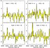 |
Fig. 3 Final CO spectra for HaR-2, HaR-1, and HaR-2-4 from run 075-14. In CO(2–1), only HaR-2 has data combined from both runs. All spectra have both polarizations combined. Spectra information and line parameters are presented in Table 2. The temperature scale corresponds to main beam temperature in mK. |
3. Results
After selecting the final spectra for every source with a visible detection and fitting their Gaussian profiles, line parameters are calculated and presented in Table 2. These CO detections present velocity centroids in the range of ~2200–2500 km s-1, and are very consistent with the HI velocities from Table 1, taken from Oosterloo & van Gorkom 2005 (their Fig. 2). H2 masses were derived from the CO(1–0) line intensity, using a Galactic CO conversion factor of 2.0 × 10²⁰ [cm-2(K km s-1)-1] and a correction factor of 1.36 to account for heavy elements ![Mathematical equation: \begin{equation} \rm {\it M}_{H_2}[{\it M}_{\odot}]=4.4\pi {\it R}^2[pc]~{\it I}_{CO(1-0)}~\left[K~km\,s^{-1}\right], \label{eq:M_H2} \end{equation}](/articles/aa/full_html/2015/10/aa26551-15/aa26551-15-eq29.png) (1)where the source’s radius R corresponds to the CO(1–0) beamsize radius at the distance of the source (17.5 Mpc from Mei et al. 2007).
(1)where the source’s radius R corresponds to the CO(1–0) beamsize radius at the distance of the source (17.5 Mpc from Mei et al. 2007).
CO detections and their line parameters.
CO(1–0) upper limits at 3σ for sources with no detection.
3.1. Star formation efficiency
To estimate how fast is the gas being transformed into stars, we compare the SFR surface density versus the gas surface density in a S-K relation, to understand the efficiency of this star formation process. Since these are low gas density regions, we can expect a large amount of gas in atomic phase, which is greater than in molecular phase. Therefore, we need to take both components, atomic and molecular, into account when estimating a total amount of gas to be converted into stars.
Molecular gas can be directly estimated from the CO(1–0) line intensity, obtained from our observations. If we take Eq. (1), and we divide it by the source area (πR2), we obtain the H2 surface density, ![Mathematical equation: \begin{equation} \rm \Sigma_{H_2}[{\it M}_{\odot}\,pc^{-2}] = 4.4 \,{\it I}_{CO(1-0)}[K~km~s^{-1}]. \label{eq:Sigma_H2} \end{equation}](/articles/aa/full_html/2015/10/aa26551-15/aa26551-15-eq43.png) (2)These values are listed in Col. 2 of Table 4 for the sources with CO(1–0) detections, including upper limits for the sources with no CO detection using Table 3.
(2)These values are listed in Col. 2 of Table 4 for the sources with CO(1–0) detections, including upper limits for the sources with no CO detection using Table 3.
For the atomic gas component, we estimated the amount of HI from the HI column density map of the NGC 4388 plume from Oosterloo & van Gorkom (2005). The atomic gas mass is derived from the integrated amount of NH inside the source solid angle, 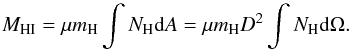 (3)Aperture photometry was done in the NH map of Oosterloo & van Gorkom (2005) to obtain the integrated column densities for our sources. We used 22′′ apertures to be consistent with our CO(1–0) observations. Since these apertures are smaller than the spatial resolution of the HI map (18 × 95.1 arcsec), the photometry results are equivalent to the pixel value of the HI map at the position of our CO targets. These values are listed in Col. 3 of Table 4. Then, by dividing Eq. (3) by the CO(1–0) beam solid angle Ω = πR2, we obtain the HI surface densities ΣHI listed in Col. 4 of Table 4.
Finally, we estimate the SFR surface density ΣSFR directly from the Hα emission in these regions. From Kennicutt & Evans (2012), ![Mathematical equation: \begin{equation} \rm log~\textit{SFR}[{\it M}_{\odot}\,yr^{-1}]=log~ \rm \textit{L}_{H_{\alpha}}[erg~ s^{-1}] - 41.27, \label{eq:SFR} \end{equation}](/articles/aa/full_html/2015/10/aa26551-15/aa26551-15-eq52.png) (4)which, divided by the CO(1–0) beam solid angle Ω, gives the SFR surface density ΣSFR. The Hα luminosities for HaR-1, HaR-2, and HaR-3-4 were obtained from Yagi et al. (2013), and are listed in Table 4, along with the corresponding ΣSFR. For the remaining sources, we used the Hα map from Kenney et al. (2008), using an aperture photometry of ~1′′ in diameter, similar to the seeing of the Hα observations from Yagi et al. (2013). For the sources with no visible detection in this map, an upper limit was calculated form the noise level of Kenney’s map, estimated in 4.8 × 10⁻⁷ erg s-1 cm-2 sr-1.
(4)which, divided by the CO(1–0) beam solid angle Ω, gives the SFR surface density ΣSFR. The Hα luminosities for HaR-1, HaR-2, and HaR-3-4 were obtained from Yagi et al. (2013), and are listed in Table 4, along with the corresponding ΣSFR. For the remaining sources, we used the Hα map from Kenney et al. (2008), using an aperture photometry of ~1′′ in diameter, similar to the seeing of the Hα observations from Yagi et al. (2013). For the sources with no visible detection in this map, an upper limit was calculated form the noise level of Kenney’s map, estimated in 4.8 × 10⁻⁷ erg s-1 cm-2 sr-1.
Schmidt-Kennicutt relation values.
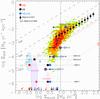 |
Fig. 4 S-K relation for sources in Table 4, with filled circles and arrows for values and upper limits, respectively. Red markers indicate H2 for Σgas, black markers HI, and blue ones the sum of both. Figure adapted from Jáchym et al. (2014), where their sources ESO137-001, 001-A, 001-B, and 001-C were plotted in a similar way as ours: red circles for H2 gas, black left arrows for HI upper limits, and blue “error bars” to account for both gas components. Colored contours account for the spiral galaxies from Bigiel et al. 2008 (green, orange, red, and purple for 1, 2, 5, and 10 sampling points per 0.05 dex, respectively). Black markers with error bars correspond to the running medians in ΣSFR as a function of σH2 of 30 nearby galaxies from Bigiel et al. (2011). Shaded ovals represent the data from the outer parts of XUV disk galaxies: NGC 4625 and NGC 6946 from Watson et al. (2014, priv. comm.), and M63 (NGC 5055) from Dessauges-Zavadsky et al. (2014), only taking H2 into account in all of them. The dashed vertical line shows the 9 M⊙ pc-2 threshold at which the atomic gas saturates. Dashed inclined lines represent “isochrones” of constant star formation efficiencies, indicating the depletion times τdep = Σgas/ ΣSFR of 108, 109, and 1010 years to consume all the gas. The dashed red isochrone marks a depletion time equal to the age of the Universe, as one Hubble time (13.8 Gyr). A representative shift of the HaR-1 marker for ΣH2 is drawn, to show the “effective” molecular gas density at which stars would form in this region if we consider a beam correction factor of +2.68 in log space, to convert our 22′′ beam to a ~1′′ beam as in the Hα data. |
The SFR surface densities are plotted as a function of the gas surface densities to construct a S-K relation in Fig. 4, using the values from Table 4. We have separately plotted, the atomic and molecular gas component of Σgas, along with a plot of both components combined, in red, black, and blue markers, respectively. Arrows denote the upper limits values from Table 4. In this figure, adapted from Jáchym et al. (2014), we can compare our sources with those of Jáchym et al. in the Norma Cluster, as well as with the sample of spiral galaxies from Bigiel et al. (2008) (in colored contours), and the sample of 30 nearby galaxies from Bigiel et al. (2011), plotted as the running medians of ΣSFR as a function of ΣH2, and with a typical depletion time of ~2.3 Gyr. Additionally, we included shaded ovals to represent regions from the outskirts of XUV disk galaxies. NGC 4625 and NGC 6946 data were taken from Watson et al. 2014 (priv. comm.), including IRAM-30 m CO observations and Hα luminosities measured within a 6′′ aperture. M63 (NGC 5055) data corresponds to the bright UV region located at 1.35r25 in Dessauges-Zavadsky et al. (2014), with IRAM 30-m CO data, and a SFR measured from the FUV and 24 μm emission.
“Isochrones” of constant star formation efficiencies are also shown to indicate the depletion times of 108, 109, and 1010 years to consume all the gas, including an additional red isochrone to mark the age of the Universe as one Hubble time (i.e., τdep = 13.8 Gyr).
Contrary to the photometry done in the HI data, the Hα data was not measured in a 22′′ diameter aperture, as the CO(1–0) FWHM, but in an aperture of 1′′ in diameter, similar to the seeing of those observations. Since we are averaging this Hα emission in a 22′′ aperture to calculate the ΣSFR, we could be diluting the real surface density of the gas being converted into stars. To correct for this beam dilution, as a representation, we shifted one of the points in Fig. 4 to a fictitious ΣH2, corresponding to a source’s solid angle of 1′′ in diameter. This correction translates in a +2.68 shift in log space, and is a representation of the real gas surface density at which stars would be formed, but it would always have the same τdep.
For Source-5, we have made the assumption that the HI and Hα emission are spatially correlated, i.e., that they both belong to the gas plume associated with NGC 4388. We know that this is true for HI, since we used the data from Oosterloo & van Gorkom (2005) and they probed the physical asociation of the HI gas plume to NGC 4388. This could not be the case for Hα, since we used the data from Kenney et al. (2008) and their Hα map show that this source could be associated with M86 instead, when Hα is considered.
From Fig. 4, we can see that our sources have extremely low SFRs in comparison with the nearby spiral galaxies, and are only comparable with the most outer clumps in the Hα/X-ray tail of the ISM stripped galaxy ESO137-001 in the Norma Cluster (Jáchym et al. 2014) and the XUV disk galaxies from Watson et al. (2014) and Dessauges-Zavadsky et al. (2014). We obtain depletion times that are significantly large. For example, HaR-1 and HaR-2 have τdep values of 2.2 × 10¹² and 1.2 × 10¹¹ years, respectively, to consume all the amount of gas present (HI + H2). These values transform into 1.6 × 10¹² and 1.0 × 10¹¹ years if we only consider the atomic gas component, and into 5.8 × 10¹¹ and 1.6 × 10¹⁰ years if we only consider the molecular component. These values are quite large in comparison with the typical τdep of ~2 Gyr for spiral galaxies, and are even larger than a Hubble time by up to 2 orders of magnitude. In Table 4, the depletion times of H2 that can be calculated are listed in Col. 7.
The extremely low SF efficiency of our sources seems to fall off the linearity of the S-K relation for typical spiral galaxies at higher gas densities, a result previously reported in other low gas density environments, such as XUV disk galaxies (Dessauges-Zavadsky et al. 2014). Watson et al. (2014) present a different conclusion for their results in XUVs, with a typical SFR in agreement with the S-K linear regime, but they take the 24 μm emission in the SFR into account, and neglect the contribution of heavy elements in the ΣH2. We see that when we correct by these differences to make their data analytically compatible with ours (i.e. neglect the 24 μm emission and correct for heavy elements), their data points in the S-K plot are comparable to ours.
4. Summary and conclusions
CO(1–0) and CO(2–1) observations were done with the IRAM 30-m telescope in a total of 11 targets all along the ram-pressure stripped tail northeast NGC 4388 in the Virgo Cluster to probe the presence of molecular gas under extreme conditions. These targets were selected for having strong peaks of HI and Hα emission.
Four of such positions showed CO detections, and three of them concentrated in the HaR-2 region, at a distance of ~70 kpc of NGC 4388, where molecular gas in unexpected. Given the large distances of these sources to NGC 4388, it is not likely that the molecular gas was stripped from the galaxy, and must have formed in situ from the HI gas plume.
Gaussian line profiles were fitted to the spectra of the detections, finding a range of velocity dispersion between 12 and 35 km s-1. The CO(1–0) line profiles were used to estimate molecular gas masses and surface densities. The amount of molecular gas in these three regions (HaR-1, HaR-2 and HaR-2-4) is very low ( between 0.7 and 2.4 × 10⁶M⊙), and their H2 surface densities between 0.2 and 0.9 M⊙ pc-2. These values are well below the HI-H2 threshold, where the gas is mainly atomic and very little is know about the SFR at these low gas densities, and, hence, the importance of these detections.
Using complementary data from Yagi et al. (2013) and Kenney et al. (2008) for Hα and from Oosterloo & van Gorkom (2005) for HI, we computed ΣSFR and ΣHI to plot, in combination with ΣH2, a S-K relation. Our sources show an extremely low SFR (up to 2 order of magnitude lower than for typical spiral galaxies). For example, HaR-1 and HaR-2 have total gas depletion times of 2.2 × 10¹² and 1.2 × 10¹¹ years, respectively. If we consider just the molecular gas component, these depletion times are 5.8 × 10¹¹ and 1.6 × 10¹⁰ years. Furthermore, Source-1 and HaR-2-4 have H2 depletion times even greater than 1.4 × 10¹² and 3.7 × 10¹¹ years respectively. These high values of depletion times exceed by far a Hubble time, thus indicating that this molecular gas will not eventually form stars, but will remain in a gaseous phase and later join the ICM.
From Fig. 4, we can see that the linearity between the SFR and the gas surface density at high gas surface densities (>9 M⊙ pc-2) for normal spiral galaxies, cannot be extrapolated to lower densities, below the HI-H2 threshold, where the star formation is extremely inefficient, and the molecular gas, even though present, does not necessarily form stars.
Acknowledgments
We warmly thank the referee for constructive comments and suggestions. Also, the IRAM staff is gratefully acknowledged for their help in the data acquisition. We thank T. Oosterloo and J. Kenney for facilitating important HI and Hα data, respectively. F.C. acknowledges the European Research Council for the Advanced Grant Program Number 267399-Momentum. We made use of the NASA/IPAC Extragalactic Database (NED), and of the HyperLeda database. C.V. acknowledges financial support from CNRS and CONICYT through agreement signed on December 11th 2007.
References
- Bigiel, F., Leroy, A., Walter, F., et al. 2008, AJ, 136, 2846 [NASA ADS] [CrossRef] [Google Scholar]
- Bigiel, F., Leroy, A. K., Walter, F., et al. 2011, ApJ, 730, L13 [NASA ADS] [CrossRef] [Google Scholar]
- Boissier, S., Gil de Paz, A., Boselli, A., et al. 2008, ApJ, 681, 244 [NASA ADS] [CrossRef] [Google Scholar]
- Boissier, S., Boselli, A., Duc, P.-A., et al. 2012, A&A, 545, A142 [NASA ADS] [CrossRef] [EDP Sciences] [Google Scholar]
- Braine, J., Lisenfeld, U., Due, P.-A., & Leon, S. 2000, Nature, 403, 867 [NASA ADS] [CrossRef] [PubMed] [Google Scholar]
- Casasola, V., Hunt, L., Combes, F., & Garcia-Burillo, S. 2015, A&A, 577, A135 [NASA ADS] [CrossRef] [EDP Sciences] [Google Scholar]
- Cayatte, V., van Gorkom, J. H., Balkowski, C., & Kotanyi, C. 1990, AJ, 100, 604 [NASA ADS] [CrossRef] [Google Scholar]
- Chung, A., van Gorkom, J. H., Kenney, J. D. P., & Vollmer, B. 2007, ApJ, 659, L115 [NASA ADS] [CrossRef] [Google Scholar]
- Chung, A., van Gorkom, J. H., Kenney, J. D. P., Crowl, H., & Vollmer, B. 2009, AJ, 138, 1741 [NASA ADS] [CrossRef] [Google Scholar]
- Cluver, M. E., Appleton, P. N., Boulanger, F., et al. 2010, ApJ, 710, 248 [NASA ADS] [CrossRef] [Google Scholar]
- Conselice, C. J., Gallagher, III, J. S., & Wyse, R. F. G. 2001, AJ, 122, 2281 [NASA ADS] [CrossRef] [Google Scholar]
- Cortese, L., Marcillac, D., Richard, J., et al. 2007, MNRAS, 376, 157 [NASA ADS] [CrossRef] [Google Scholar]
- Dasyra, K. M., Combes, F., Salomé, P., & Braine, J. 2012, A&A, 540, A112 [NASA ADS] [CrossRef] [EDP Sciences] [Google Scholar]
- Davies, J. I., Bianchi, S., Cortese, L., et al. 2012, MNRAS, 419, 3505 [NASA ADS] [CrossRef] [Google Scholar]
- DeMaio, T., Gonzalez, A. H., Zabludoff, A., Zaritsky, D., & Bradač, M. 2015, MNRAS, 448, 1162 [NASA ADS] [CrossRef] [Google Scholar]
- Dessauges-Zavadsky, M., Verdugo, C., Combes, F., & Pfenniger, D. 2014, A&A, 566, A147 [NASA ADS] [CrossRef] [EDP Sciences] [Google Scholar]
- Edge, A. C., Oonk, J. B. R., Mittal, R., et al. 2010, A&A, 518, L46 [NASA ADS] [CrossRef] [EDP Sciences] [Google Scholar]
- Fabian, A. C., Sanders, J. S., Taylor, G. B., et al. 2006, MNRAS, 366, 417 [Google Scholar]
- Feldmeier, J. J., Mihos, J. C., Morrison, H. L., Rodney, S. A., & Harding, P. 2002, ApJ, 575, 779 [NASA ADS] [CrossRef] [Google Scholar]
- Ferland, G. J., Fabian, A. C., Hatch, N. A., et al. 2009, MNRAS, 392, 1475 [NASA ADS] [CrossRef] [Google Scholar]
- Gavazzi, G., Boselli, A., Mayer, L., et al. 2001, ApJ, 563, L23 [NASA ADS] [CrossRef] [Google Scholar]
- Gu, L., Yagi, M., Nakazawa, K., et al. 2013, ApJ, 777, L36 [NASA ADS] [CrossRef] [Google Scholar]
- Gunn, J. E., & Gott, III, J. R. 1972, ApJ, 176, 1 [NASA ADS] [CrossRef] [Google Scholar]
- Iwasawa, K., Wilson, A. S., Fabian, A. C., & Young, A. J. 2003, MNRAS, 345, 369 [NASA ADS] [CrossRef] [Google Scholar]
- Jáchym, P., Palouš, J., Köppen, J., & Combes, F. 2007, A&A, 472, 5 [NASA ADS] [CrossRef] [EDP Sciences] [Google Scholar]
- Jáchym, P., Combes, F., Cortese, L., Sun, M., & Kenney, J. D. P. 2014, ApJ, 792, 11 [NASA ADS] [CrossRef] [Google Scholar]
- Kenney, J. D. P., & Young, J. S. 1989, ApJ, 344, 171 [NASA ADS] [CrossRef] [Google Scholar]
- Kenney, J. D. P., van Gorkom, J. H., & Vollmer, B. 2004, AJ, 127, 3361 [NASA ADS] [CrossRef] [Google Scholar]
- Kenney, J. D. P., Tal, T., Crowl, H. H., Feldmeier, J., & Jacoby, G. H. 2008, ApJ, 687, L69 [NASA ADS] [CrossRef] [Google Scholar]
- Kennicutt, R. C., & Evans, N. J. 2012, ARA&A, 50, 531 [NASA ADS] [CrossRef] [Google Scholar]
- Leroy, A. K., Walter, F., Sandstrom, K., et al. 2013, AJ, 146, 19 [NASA ADS] [CrossRef] [Google Scholar]
- Lim, J., Ohyama, Y., Chi-Hung, Y., Dinh-V-Trung, & Shiang-Yu, W. 2012, ApJ, 744, 112 [NASA ADS] [CrossRef] [Google Scholar]
- Machacek, M. E., Jones, C., & Forman, W. R. 2004, ApJ, 610, 183 [NASA ADS] [CrossRef] [Google Scholar]
- Machacek, M., Dosaj, A., Forman, W., et al. 2005, ApJ, 621, 663 [NASA ADS] [CrossRef] [Google Scholar]
- Mahdavi, A., Geller, M. J., Fabricant, D. G., et al. 1996, AJ, 111, 64 [NASA ADS] [CrossRef] [Google Scholar]
- Mei, S., Blakeslee, J. P., Côté, P., et al. 2007, ApJ, 655, 144 [NASA ADS] [CrossRef] [Google Scholar]
- Merritt, D. 1984, ApJ, 276, 26 [NASA ADS] [CrossRef] [Google Scholar]
- Mihos, J. C., Harding, P., Feldmeier, J., & Morrison, H. 2005, ApJ, 631, L41 [NASA ADS] [CrossRef] [Google Scholar]
- Nulsen, P. E. J. 1982, MNRAS, 198, 1007 [NASA ADS] [CrossRef] [Google Scholar]
- Oosterloo, T., & van Gorkom, J. 2005, A&A, 437, L19 [NASA ADS] [CrossRef] [EDP Sciences] [Google Scholar]
- O’Sullivan, E., Giacintucci, S., Vrtilek, J. M., Raychaudhury, S., & David, L. P. 2009, ApJ, 701, 1560 [NASA ADS] [CrossRef] [Google Scholar]
- Quilis, V., Moore, B., & Bower, R. 2000, Science, 288, 1617 [NASA ADS] [CrossRef] [PubMed] [Google Scholar]
- Roediger, E., & Hensler, G. 2005, A&A, 433, 875 [NASA ADS] [CrossRef] [EDP Sciences] [Google Scholar]
- Salomé, P., Combes, F., Edge, A. C., et al. 2006, A&A, 454, 437 [NASA ADS] [CrossRef] [EDP Sciences] [Google Scholar]
- Salomé, P., Combes, F., Revaz, Y., et al. 2011, A&A, 531, A85 [NASA ADS] [CrossRef] [EDP Sciences] [Google Scholar]
- Scott, T. C., Cortese, L., Brinks, E., et al. 2012, MNRAS, 419, L19 [NASA ADS] [CrossRef] [Google Scholar]
- Serra, P., Koribalski, B., Duc, P.-A., et al. 2013, MNRAS, 428, 370 [NASA ADS] [CrossRef] [Google Scholar]
- Sun, M., Donahue, M., & Voit, G. M. 2007, ApJ, 671, 190 [NASA ADS] [CrossRef] [Google Scholar]
- Sun, M., Donahue, M., Roediger, E., et al. 2010, ApJ, 708, 946 [NASA ADS] [CrossRef] [Google Scholar]
- Tamura, T., Maeda, Y., Mitsuda, K., et al. 2009, ApJ, 705, L62 [NASA ADS] [CrossRef] [Google Scholar]
- Tonnesen, S., Bryan, G. L., & van Gorkom, J. H. 2007, ApJ, 671, 1434 [NASA ADS] [CrossRef] [Google Scholar]
- Vollmer, B., Cayatte, V., Balkowski, C., & Duschl, W. J. 2001, ApJ, 561, 708 [NASA ADS] [CrossRef] [Google Scholar]
- Vollmer, B., Braine, J., Combes, F., & Sofue, Y. 2005, A&A, 441, 473 [NASA ADS] [CrossRef] [EDP Sciences] [Google Scholar]
- Vollmer, B., Beckert, T., & Davies, R. I. 2008, A&A, 491, 441 [NASA ADS] [CrossRef] [EDP Sciences] [Google Scholar]
- Watson, L. C., Martini, P., Lisenfeld, U., et al. 2014, in AAS Meet. Abst., 223, 454.22 [Google Scholar]
- Yagi, M., Komiyama, Y., Yoshida, M., et al. 2007, ApJ, 660, 1209 [NASA ADS] [CrossRef] [Google Scholar]
- Yagi, M., Gu, L., Fujita, Y., et al. 2013, ApJ, 778, 91 [NASA ADS] [CrossRef] [Google Scholar]
- Yoshida, M., Yagi, M., Okamura, S., et al. 2002, ApJ, 567, 118 [NASA ADS] [CrossRef] [Google Scholar]
- Zhang, B., Sun, M., Ji, L., et al. 2013, ApJ, 777, 122 [NASA ADS] [CrossRef] [Google Scholar]
All Tables
All Figures
|
Fig. 1 Targets observed in the Virgo Cluster. Orange: HI contours levels at 1, 5, 10 and 50 × 1019 cm-2 from Oosterloo & van Gorkom (2005), showing the plume of atomic gas stripped from NGC 4388. Purple: Hα contours levels at 5, 11, and 50 e−/s (Kenney et al. 2008). Cyan: 250 μm contour levels at 0.01 and 0.1 Jy/beam (Davies et al. 2012). In zoomed regions: targets selected close to HaR-2 for run 075-14 (red circles). Circles enclosing targets are 22′′ width, as the CO(1–0) HPBW. |
| In the text | |
|
Fig. 2 Top: spectra taken at the center of NGC 4388, observed for calibration purposes. Bottom: spectra from observing run 195-13, which showed CO emission. Spectra information and line parameters are presented in Table 2. The temperature scale corresponds to main beam temperature in mK. |
| In the text | |
|
Fig. 3 Final CO spectra for HaR-2, HaR-1, and HaR-2-4 from run 075-14. In CO(2–1), only HaR-2 has data combined from both runs. All spectra have both polarizations combined. Spectra information and line parameters are presented in Table 2. The temperature scale corresponds to main beam temperature in mK. |
| In the text | |
|
Fig. 4 S-K relation for sources in Table 4, with filled circles and arrows for values and upper limits, respectively. Red markers indicate H2 for Σgas, black markers HI, and blue ones the sum of both. Figure adapted from Jáchym et al. (2014), where their sources ESO137-001, 001-A, 001-B, and 001-C were plotted in a similar way as ours: red circles for H2 gas, black left arrows for HI upper limits, and blue “error bars” to account for both gas components. Colored contours account for the spiral galaxies from Bigiel et al. 2008 (green, orange, red, and purple for 1, 2, 5, and 10 sampling points per 0.05 dex, respectively). Black markers with error bars correspond to the running medians in ΣSFR as a function of σH2 of 30 nearby galaxies from Bigiel et al. (2011). Shaded ovals represent the data from the outer parts of XUV disk galaxies: NGC 4625 and NGC 6946 from Watson et al. (2014, priv. comm.), and M63 (NGC 5055) from Dessauges-Zavadsky et al. (2014), only taking H2 into account in all of them. The dashed vertical line shows the 9 M⊙ pc-2 threshold at which the atomic gas saturates. Dashed inclined lines represent “isochrones” of constant star formation efficiencies, indicating the depletion times τdep = Σgas/ ΣSFR of 108, 109, and 1010 years to consume all the gas. The dashed red isochrone marks a depletion time equal to the age of the Universe, as one Hubble time (13.8 Gyr). A representative shift of the HaR-1 marker for ΣH2 is drawn, to show the “effective” molecular gas density at which stars would form in this region if we consider a beam correction factor of +2.68 in log space, to convert our 22′′ beam to a ~1′′ beam as in the Hα data. |
| In the text | |
Current usage metrics show cumulative count of Article Views (full-text article views including HTML views, PDF and ePub downloads, according to the available data) and Abstracts Views on Vision4Press platform.
Data correspond to usage on the plateform after 2015. The current usage metrics is available 48-96 hours after online publication and is updated daily on week days.
Initial download of the metrics may take a while.