| Issue |
A&A
Volume 582, October 2015
|
|
|---|---|---|
| Article Number | A73 | |
| Number of page(s) | 19 | |
| Section | Stellar structure and evolution | |
| DOI | https://doi.org/10.1051/0004-6361/201526408 | |
| Published online | 12 October 2015 | |
The VLT-FLAMES Tarantula Survey
XXIII. Two massive double-lined binaries in 30 Doradus⋆,⋆⋆
1 Department of Physics & Astronomy, University College London, Gower Street, London, WC1E 6BT, UK
2 Astrophysics Research Centre, Queen’s University Belfast, BT7 1NN, Northern Ireland, UK
3 UK Astronomy Technology Centre, Royal Observatory Edinburgh, Blackford Hill, Edinburgh, EH9 3HJ, UK
4 Department of Physics & Astronomy, Johns Hopkins University, Bloomberg Center for Physics and Astronomy, Room 520, 3400 N. Charles Street, Baltimore, MD 21218, USA
5 Instituto de Astronomia, Geofísica e Ciências, Rua do Matão 1226, Cidade Universitária São Paulo, 05508-090 São Paulo SP, Brasil
6 IAASARS, National Observatory of Athens, 15236 Penteli, Greece
7 Department of Physics & Astronomy, The Open University, Walton Hall, Milton Keynes, MK7 6AA, UK
8 Argelander Institut für Astronomie der Universität Bonn, Auf dem Hügel 71, 53121 Bonn, Germany
9 ESA/STScI, 3700 San Martin Drive, Baltimore, MD 21218, USA
10 Instituto de Astrofísica de Canarias, 38200 La Laguna, Tenerife, Spain
11 Departamento de Astrofísica, Universidad de La Laguna, 38205 La Laguna, Tenerife, Spain
12 Warsaw University Observatory, Al. Ujazdowskie 4, 00-478 Warszawa, Poland
Received: 25 April 2015
Accepted: 24 August 2015
Abstract
Aims. We investigate the characteristics of two newly discovered short-period, double-lined, massive binary systems in the Large Magellanic Cloud, VFTS 450 (O9.7 II–Ib + O7::) and VFTS 652 (B1 Ib + O9: III:).
Methods. We perform model-atmosphere analyses to characterise the photospheric properties of both members of each binary (denoting the “primary” as the spectroscopically more conspicuous component). Radial velocities and optical photometry are used to estimate the binary-system parameters.
Results. We estimate Teff = 27 kK, log g = 2.9 (cgs) for the VFTS 450 primary spectrum (34 kK, 3.6: for the secondary spectrum); and Teff = 22 kK, log g = 2.8 for the VFTS 652 primary spectrum (35 kK, 3.7: for the secondary spectrum). Both primaries show surface nitrogen enrichments (of more than 1 dex for VFTS 652), and probable moderate oxygen depletions relative to reference LMC abundances. We determine orbital periods of 6.89 d and 8.59 d for VFTS 450 and VFTS 652, respectively, and argue that the primaries must be close to filling their Roche lobes. Supposing this to be the case, we estimate component masses in the range ~20–50 M⊙.
Conclusions. The secondary spectra are associated with the more massive components, suggesting that both systems are high-mass analogues of classical Algol systems, undergoing case-A mass transfer. Difficulties in reconciling the spectroscopic analyses with the light-curves and with evolutionary considerations suggest that the secondary spectra are contaminated by (or arise in) accretion disks.
Key words: binaries: eclipsing / binaries: close / binaries: spectroscopic
Based on observations obtained at the European Southern Observatory Very Large Telescope (VLT) as part of programmes 182.D-0222 and 090.D-0323.
Tables 2, 3, and 8 are available in electronic form at http://www.aanda.org
© ESO, 2015
1. Introduction
Massive, luminous stars are of interest for the role that they play in galactic chemical evolution; the environmental impact they have through mechanical and radiative energy input to their surroundings; and as tracers of recent star formation. However, while there have been considerable advances in modelling their spectra, direct determinations of their fundamental parameters are relatively few, because of the scarcity of suitable double-lined eclipsing binary systems (cf., e.g., Bonanos 2009, and references therein).
Multi-epoch spectroscopy from the VLT-FLAMES Tarantula Survey (VFTS; Evans et al. 2011) of the OB-star population of 30 Doradus, in the Large Magellanic Cloud (LMC), has led to the discovery of a number of systems showing radial-velocity variations that appear to be consistent with binary motion (Sana et al. 2013; Dunstall et al. 2015). These systems offer an important opportunity to better understand the physical properties of stars in the upper Hertzsprung-Russell diagram, as exemplified by the VFTS study of R139 by Taylor et al. (2011).
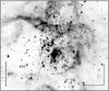 |
Fig. 1 Central region of 30 Dor, showing R136 and the locations of VFTS 450 and VFTS 652. |
Here we discuss two newly identified double-lined radial-velocity variables discovered in the VFTS: Nos. 450 and 652 (stars 50 and 5 in Melnick 1985). The primary velocity amplitudes are among the largest measured in the VFTS dataset, and the number of spectroscopic observations available makes it possible to undertake full orbital analyses (rather than mere detections of variability). Each system also shows orbital photometric variability. Both are relatively close to the core of 30 Dor, with radial distances of 0.́47 and 0.́83 from R136 (Fig. 1), corresponding to projected distances of 6.8 and 12.0 pc, respectively.
The paper is organized as follows: Sect. 2 summarizes the data, and the binary characteristics are examined in Sect. 3. A model-atmosphere analysis is described in Sect. 4, and simple models of the systems are constructed in Sect. 5. Throughout the paper we adopt the convention that the “primary” in each system is the star with the stronger optical absorption-line spectrum (though we shall argue that this is probably not the more massive component).
Characteristics of spectroscopic observations.
Basic observed properties.
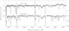 |
Fig. 2 Rectified blue-region spectra of VFTS 450 and 652, velocity shifted to the rest frame of the primary. The data are LR02 and LR03 spectra from MJD 54 748, 54 810 (VFTS 450; φ ≃ 0.12 from the circular-orbit ephemeris in Table 5) and 56 294, 54 808 (VFTS 652, φ ≃ 0.66), merged at ~4560 Å. Secondary spectra are offset by ca. +260, −150 kms-1 (VFTS 450, 652, respectively). Narrow Balmer emission is nebular. |
2. Observations
2.1. Optical Spectroscopy
Initial spectroscopic data were obtained as part of the VFTS (Evans et al. 2011), using the Fibre Large Array Multi-Element Spectrograph (FLAMES; Pasquini et al. 2002) on the Very Large Telescope, primarily with the Giraffe spectrograph, but with supplementary data from the Ultraviolet and Visual Echelle Spectrograph (UVES). These observations were obtained in the 2008/9 and 2009/10 observing seasons; additional Giraffe spectroscopy was secured as part of a binary-monitoring campaign of VFTS targets between 2012 Oct. and 2013 Mar.
Table 1 summarizes the basic instrumental characteristics; a full account of the observations and data reduction is given by Evans et al. (2011). Logs of the individual blue-region spectra, which are the principal focus of this paper, are given in Tables 2 and 3. Representative spectra are shown in Fig. 2.
2.1.1. Spectral types
Spectral types previously determined from the VFTS spectra are O9.7 III: + O7:: and B2 Ip + O9 III: (VFTS 450, VFTS 652; Walborn et al. 2014). Melnick (1985) gives O9.5 I and O9.5 V pec (“binary?”) for VFTS 450 and 652, respectively, while Walborn & Blades (1997) report ON9: I and B2 Ib.
Our review of the more extensive dataset discussed here, including examination of the disentangled component spectra presented in Sect. 3.3, broadly supports the Walborn et al. (2014) classifications, but the clear presence of Si iv λ4089 and λ4116 in the primary spectrum of VFTS 652 leads us to revise its classification to B1 Ib. The crucial He iλ4471 classification line suffers significant nebular contamination in the disentangled secondary spectra, admitting the possibility of an O8 (or, conceivably, O7) secondary spectrum for this target.
Our rectification of the VFTS 450 spectra leaves a broad, shallow emission feature spanning λλ4640, 4686 (C iii/N iii, He ii; Fig. 2). We have investigated, and rejected, possible instrumental origins, including contamination by the nearby WR star Brey 79 (3.̋5 distant). While such features are not widely reported, and are easily overlooked, they are not unprecedented in late-O supergiants (e.g., α Cam, O9 Ia; Wilson 1958); this suggests the possibility of a brighter luminosity class for the VFTS 450 primary than previously inferred from VFTS data. The intensity of the Si iv lines compared to He i λ4026 also indicates a somewhat more luminous type (cf. Table 6 of Sota et al. 2011). The arbitrary intensity scaling of the disentangled spectrum hampers a precise assignment, but we revise the previous classification for the VFTS 450 primary spectrum to O9.7 II−Ib1. Our adopted spectral types are incorporated into Table 4.
2.1.2. Hα spectra
We have Hα observations, shown in Fig. 3, at a single epoch for each system. These spectra suffer from strong nebular contamination which is poorly corrected by standard sky subtraction, but nevertheless each star clearly shows broad, double-peaked intrinsic emission. Although the single-epoch spectra may not be representative of typical behaviour, this emission morphology is characteristic of interacting binaries, rather than typical OB-star stellar-wind P Cygni profiles. Peak-to-peak separations are ~560 and 420 kms-1 for VFTS 450 and 652, respectively, with full widths at continuum level about twice those values.
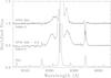 |
Fig. 3 Hα spectra, labelled with MJDs of mid-observation. The subtracted sky spectrum is shown for reference, and illustrates the nebular contamination, which varies on small spatial scales; correction for this nebular emission in the stellar spectra is generally poor, in particular in the residual core Hα emission, although the extended double-peaked emission is real. |
2.2. Photometry
2.2.1. OGLE photometry
We have OGLE IC-band photometry from phases III and IV of the project (cf. Udalski et al. 2008, 2015), spanning 2001 October to 2009 April and 2010 March to 2014 March, respectively. Each dataset for each star consists of ~400 observations. We have also examined the sparser OGLE-III V-band data.
VFTS 450 is located in a high-background region, and, as noted above, is only ~3.̋5 arcsec from Brey 79 (IC ≃ 12.7). The standard OGLE-III Difference Image Analysis (DIA) pipeline is not optimal under these circumstances, and we found that a profile-fitting extraction, using DoPhot (Schechter et al. 1993), resulted in reduced scatter. Furthermore, the OGLE-IV IC photometry for this target is ~0 17 brighter than the OGLE-III data (regardless of extraction method). This is probably a consequence of the high background; while it is difficult to be certain, we believe the OGLE-IV normalization to be the more reliable. Neither issue arises in the VFTS 652 results.
Both stars show orbital photometric variability, with full amplitudes of ~02. Periods were determined by using a date-compensated discrete fourier transform (Ferraz-Mello 1981), augmented with least-squares fitting of a double sine wave. Results are included in Table 5. There are no significant differences in periods determined from the OGLE-III, OGLE-IV, and combined datasets (Table 5 gives results from the combined IC-band data). The phased OGLE photometry is shown in Fig. 5. The rms scatter about the mean curve for VFTS 450, ~0023, is consistent with the probable measurement uncertainties, but the larger scatter for VFTS 652, ~0036, suggests significant intrinsic variability.
 |
Fig. 4 Colour–magnitude diagram, comparing VFTS 450 and 652 to selected LMC emission-line stars and OBA supergiants (after Bonanos et al. 2009). |
 |
Fig. 5 OGLE photometry. Phases are computed with respect to the photometric circular-orbit T0 values and periods reported in Table 5. OGLE-III and OGLE-IV magnitudes are shown in grey and black, respectively; the OGLE-III results for VFTS 450 have been offset by |

2.2.2. IR photometry
Representative visual–IR magnitudes for both stars, adapted from the compilation by Bonanos et al. (2009), are listed in Table 4, and are included in a J− [3.6] , [3.6] colour–magnitude diagram of luminous LMC sources in Fig. 4. VFTS 652 lies at the red edge of the distribution of normal OBA supergiants in this figure (though this displacement from the main grouping could possibly arise from different phase sampling at J and [3.6] of the orbital photometric variability discussed in Sect. 3.2). However, at these wavelengths VFTS 450 has a substantial IR excess, intermediate between those of typical Wolf-Rayet stars and supergiant B[e] stars.
3. Spectroscopic orbits
3.1. Radial-velocity measurements
3.1.1. Primaries
Radial velocities for the primary components were reasonably straightforward to measure using relatively unblended Si iii and He i lines. We used the results of the model-atmosphere analyses reported in Sect. 4 to identify suitable tlusty models to employ as templates in a cross-correlation analysis. Results, which are insensitive to the precise choice of model template, are incorporated into Tables 2 and 3; the dispersion in velocities from different lines, and residuals from the orbital solutions discussed in Sect. 3.2, are consistent with measurement errors of ≲10 kms-1.
3.1.2. Secondaries
In order to measure the much weaker secondary spectra, we merged LR02/LR03 spectra taken on any given night using a weighted mean, with a sigma-clipping algorithm to exclude cosmic-ray events and other flaws. (Multiple observations taken at a given spectrograph setting on any one night span ≲1% of the orbital periods that we report in Table 5, and may therefore be combined without special procedures to compensate for binary motion.) Uncertain corrections for echelle blaze render measurements in the UVES spectra unreliable.
The secondary velocities were measured by direct fitting of gaussians, but the shallowness and breadth of the lines make the results quite sensitive to the adopted rectification. Repeat measurements and residuals to model fits are both consistent with typical measurement errors of ~35 kms-1.
VFTS 450.
Because of blending with features in the primary spectrum, we did not attempt radial-velocity measurements of the secondary at phases near conjunctions (100 ≲ Vprimary ≲ 400kms-1). The helium lines in the secondary spectrum show poor agreement, as illustrated in Fig. 6; the He iiλ4200 velocities are generally – though not consistently – some ~100 kms-1 more positive than found for He iiλ4541 or He i λ4471. Given the shallowness of the lines in the secondary spectra, we cannot rule out that rectification difficulties contribute to this problem. In practice, we rely principally on results for λ4200, which gives consistent results and which is not subject to significant blending (cp., e.g., secondary λ4541, which can be affected by Si iiiλ4552 in the primary spectrum).
VFTS 652.
The absence of He ii lines in the primary spectrum renders measurement of the weak He iiλ4541 line in the secondary reasonably straightforward in both LR02 and LR03 spectra. He iiλ4200 gives consistent, but somewhat more scattered, results.
 |
Fig. 6 Selected helium lines in the spectrum of VFTS 450 near quadrature; smooth red curves show gaussian fits to the data. Although these helium lines give consistent results for the primary (at ~+400 kms-1), the secondary velocities are discordant (Sect. 3.1.2; for reference, the dashed vertical line indicates the measured secondary He iλ4471 velocity). This figure also illustrates the differences in He i:He ii line ratios in the two components (Sect. 4.2). |
Radial-velocity orbital solutions, for circular and eccentric orbits.
3.2. Results
The primaries’ spectroscopic orbits are summarized in Table 5, and are illustrated in Figs. 8 and 9. We adopted uniform weighting for our final solutions, but other weighting schemes result in unimportant changes to the orbital parameters. According to the formulation of the F test described by Lucy & Sweeney (1971), the orbital eccentricities are formally significant with >99% confidence. However, the apparent eccentricities are quite small, and we caution that they may not reflect the true centre-of-mass motions.
Given the considerable uncertainties in the radial-velocity measurements of the secondaries, we chose a simple but robust method to estimate the mass ratio for each system, namely, a linear regression of the secondary velocities on the primary values (Fig. 10). The gradient yields the mass ratio directly, independently of all other parameters; results are included in Table 5. The means of the observed minus predicted secondary orbital velocities (i.e., the differences between primary and secondary γ velocities) are +10.0 ± 8.5 (s.e.) and +29.5 ± 6.5kms-1 for VFTS 450 and 652, respectively; differences in γ velocities such as that shown by VFTS 652 have been found previously in “windy” massive binaries (e.g., Niemela & Morrell 1986; Niemela & Bassino 1994).
Although the spectroscopic period determined for VFTS 450 differs from the photometric value by ~1.7σ, we don’t consider this to be significant evidence for period changes, given that the OGLE-III and OGLE-IV datasets are in good mutual agreement, and span the spectroscopic epochs.
3.3. Disentangling
In principle, an alternative approach to the spectroscopic-orbit modelling is a simultaneous solution of the individual component spectra and the orbital characteristics (“disentangling”; cf., e.g., Hadrava 2004). Because of the weakness of the secondary spectra we instead chose the simpler option of reconstructing the separate component spectra in the more extensive LR02 datasets from the “known” velocities, using cres (Ilijić 2004). We explored the consequences of using observed velocities or those calculated from the orbital solution, including using mass ratios in the range 0.5–1.0 when computing the secondary spectra. We found the results to be quite robust to these factors (the corollary being that the technique cannot recover a precise mass ratio for these data). The resulting spectra of individual components are shown in Fig. 11; they have better S:N than any individual spectrum, but the y scaling is arbitrary, and nebular emission contaminates some key lines.
4. Model-atmosphere analysis
4.1. Methodology
Model-atmosphere analyses of both systems were performed using a grid of line-blanketed non-LTE tlusty models at LMC metallicity (Hubeny 1988; Hubeny & Lanz 1995; Hubeny et al. 1998; for more details of the grid see Ryans et al. 2003; Dufton et al. 2005). The analyses assume that each component’s spectrum can be reliably characterized by a single set of atmospheric parameters, and that hydrostatic, plane-parallel structures are appropriate. Depending on the adequacy or otherwise of these assumptions, the results may be subject to significant (and largely unquantifiable) systematic errors, and should therefore be interpreted with due caution.
For the primary spectra, the atmospheric parameters were estimated from the Si iii and Si iv line strengths, together with the H i and He ii profiles. The lower quality of the secondary spectra allowed only relatively rough estimates of parameter values to be made, using the H i and He ii lines; the microturbulence was indeterminate (and unimportant) for these lines, and we assumed appropriate values.
The analyses were based principally on the disentangled spectra, which have better signal:noise ratios than any individual spectrum (and, of course, should be free from blending), although cross-checks were made against the directly observed spectra, particularly for the Balmer lines, which suffer nebular contamination.
A complication is the uncertainty in the relative flux contributions of the two components in each system; without ancillary information, it is impossible to distinguish between a strong continuum with weak lines and a weak continuum with strong lines. We addressed this issue by supposing that the primary [secondary] contributes a wavelength-independent fraction ℱ1 [ℱ2, = 1−ℱ1] of the rectified continuum flux, and adjusted this fraction as necessary.
Equivalent widths of the primary in the integrated spectra.
4.1.1. Metal-line equivalent widths
The data quality allows abundance analyses to be conducted for the primary spectra. For this purpose, equivalent widths were measured by fitting theoretical profiles to the observations, using a least-squares technique. In the LR03 region directly observed spectra were used; for the LR02 setting, the disentangled spectra were employed (to take advantage of the improved S/N), and the results scaled to recover the Wλ values that would be determined in the directly observed spectra. Results are summarized in Table 6.
The λ4552 Si iii line falls in the region of overlap between LR02 and LR03 spectra; results from both spectrograph configurations are separately listed in the Table. The values from the two settings differ by ~15 mÅ, in opposite senses for VFTS 450 and VFTS 652. This is probably a fair reflection of observational uncertainties (including, potentially, temporal/orbital variations, although comparison of LR02 spectra taken at different epochs shows no evidence for substantial changes in line strengths).
The disentangling results show that the absorption lines of metals can be safely attributed to the primary spectra (even in the LR03 data), but of course the measurements in Table 6 have to be scaled by the appropriate ℱ value when performing an abundance analysis.
4.2. VFTS 450
The LR02 primary spectrum shows hydrogen and neutral & ionized helium lines, together with strong metal lines (particularly O ii and Si iv). By contrast, only the hydrogen and ionized helium lines are clearly seen in the secondary spectrum, with the former being badly contaminated by nebular emission. The He i lines at 4387, 4471 Å are probably present, with less convincing evidence for Si iv λ4089 and N iii λλ4097, 4510–4534.
Summary of stellar-atmosphere parameter determinations.
Primary:
the primary spectrum was first analysed by assuming no secondary contamination (i.e., ℱ2 ≡ 0), leading to estimates of Teff and log g that are, in practice, lower limits to allowable values. To investigate the sensitivity of the results to spectral contamination by the secondary component, the analysis was repeated for ℱ2 = 0.25, 0.5, spanning the range of plausible values; results are summarized in Table 7.
Gravities were estimated from the Hδ and Hγ line profiles, with results agreeing to better than 0.1 dex. The effective temperature was estimated from the He ii spectrum (by assuming a normal helium abundance), as results from the silicon ionization equilibrium were found to be sensitive to the microturbulence, ξ, and were used to determine that parameter. (Because of the relatively large value of ξ, the Si iii triplet lines at 4552−4574 Å lie near the linear part of the curve of growth, and hence are not particularly sensitive to the microturbulence.)
Given ξ and ℱ, element abundances were estimated from the equivalent widths listed in Table 6, with standard deviations of 0.1−0.2 dex implied by the individual oxygen estimates. To obtain approximately “normal” LMC abundances for magnesium and silicon requires ℱ2 ≃ 0.25, which represents our “best-bet” model. There then appears to be a significant surface-nitrogen enhancement approaching 1 dex, and an oxygen depletion of ~0.3 dex.
The range of parameter estimates, together with the agreement between theoretical and observed profiles, leads us to adopt modelling uncertainties of ±1 kK in Teff, ±0.2 dex in log g, and 2 kms-1 in ξ. Uncertainties on the abundances are difficult to address precisely; the adopted uncertainties in the atmospheric parameters alone translate into typical errors of 0.15 dex for both nitrogen and oxygen, (see Hunter et al. 2007 for more details). Varying the secondary contribution (ℱ2) contributes significant additional uncertainty to the absolute abundances, but has little effect on the N:O abundance ratio; the inference of a significant surface-nitrogen enhancement appears to be robust.
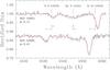 |
Fig. 7 VFTS 652 as a double-lined spectroscopic binary (Sect. 4.3). Wavelengths of selected lines are shown in the rest frame of the system centre of mass, together with the observed orbital displacements of N iiλ4530, Si iiiλ4552 (primary spectrum), and He iiλ4541 (secondary spectrum). |
Secondary:
the weakness of the secondary’s absorption lines makes an atmospheric analysis difficult, and our results should be treated with caution. Nonetheless, the He ii absorption lines do provide useful diagnostics, principally for the effective temperature. Additionally, although the Balmer-series lines are badly contaminated by nebular emission, the lack of significant Stark-broadened wings sets an upper limit on the surface gravity. As an exercise in defining the range of possible parameter space, we conducted analyses assuming that the continuum was entirely due to the secondary (ℱ2 = 1), along with two cases considered for the primary (ℱ2 = 0.25 and 0.5); the results are summarized in Table 7. Note that the gravity limits are appropriate for the upper limit of the effective-temperature range – a lower effective temperature would lead to lower gravity limit.
4.3. VFTS 652
The spectra of VFTS 652 show a rich metal-line spectrum for the primary, in accord with its classification as a B-type supergiant. The secondary spectrum shows convincing evidence for the presence of He ii lines (Fig. 7), together with Stark-broadened wings in the Balmer series; He i lines also appear to be present.
Primary:
as for VFTS 450, we evaluated parameters for ℱ2 = 0, 0.25, and 0.5. The effective temperature was estimated from the silicon ionization equilibrium, the gravity from the Balmer-line profiles, and the microturbulence from the relative strengths of lines in the Si iii triplet. Results are summarized in Table 7.
To obtain “normal” LMC abundances for magnesium and silicon requires ℱ2 = 0.25–0.50. Abundances were also derived for nitrogen and oxygen, with the scatter among estimates from individual lines being in the range 0.1–0.2 dex. Using the same criteria as for VFTS 450 leads to estimated uncertainties of ±1 kK, ±0.1 dex, and ±3 kms-1, for Teff, log g, and ξ respectively. These in turn imply uncertainties of typically 0.2–0.3 dex for the nitrogen and oxygen abundances (but significantly less for the N:O abundance ratio). The effects of varying the dilution factor are relatively small, leading to adopted final errors of 0.3 dex for these elements; a conservative error estimate on the N:O ratio is ~0.2 dex.
At ℱ2 = 0.25, the oxygen abundance is possibly underabundant, by ~0.4 dex compared to the LMC baseline, while nitrogen is again clearly enhanced, by more than 1.0 dex. Qualitatively similar conclusions follow for other dilution factors; regardless of the dilution factor adopted, the N:O abundance ratio is 1.6–1.7 dex higher than for the adopted LMC baseline abundances.
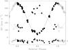 |
Fig. 8 Spectroscopic orbit for VFTS 450; orbital phases refer to the circular-orbit T0 (from Table 5), as do the (O−C) residuals for the primary shown at the bottom of the plot. The eccentric-orbit solution for the primary is shown as a dotted line (which may appear as a continuous grey line if viewed at low resolution), and the circular orbit for the secondary as a dash-dot line. Diamonds show the He iiλ4200 velocities measured in the secondary’s spectrum, and used to estimate the mass ratio. |
 |
Fig. 9 Spectroscopic orbit for VFTS 652; details as for Fig. 8, except that He iiλ 4541 velocities are shown for the secondary. |
 |
Fig. 10 Spectroscopic mass-ratio determination; secondary velocities have been offset as indicated for display purposes (primary velocities unchanged). The slope of the linear fit gives the mass ratio directly. |
Secondary:
again as an exercise in defining the range of possible parameter space, we used the He ii λλ4200, 4541 and available Balmer lines to estimate atmospheric parameters for several dilution factors. The results are summarized in Table 7; for ℱ2 = 0.25, inferred stellar parameters lie at the boundary of, or just outside, our grid of tlusty models. Representative values of the microturbulence were adopted but varying these by reasonable amounts would have a negligible effect on our estimates.
The absence of detectable metal lines in the secondary spectrum is consistent with the adopted parameters, secondary flux level, and signal:noise ratio.
 |
Fig. 11 Disentangled component spectra; the y-axis scaling is approximate (and depends on the primary:secondary continuum flux ratios). The Balmer lines and, to a lesser extent, He i are corrupted by nebular emission (marked as “n”); broad features, such as the λ4430 diffuse interstellar band, are rectified out. |
4.4. Uncertainties
Atmospheric parameters:
the primary spectrum of VFTS 652 was easier to model than that of VFTS 450, with better internal agreement between different spectral features. However, for both systems the inclusion of dilution by the secondary leads to only relatively small changes in fit parameters. We therefore expect the error estimates for the primaries’ Teff and log g values discussed above to be reasonable.
Parameter estimates for the secondary components are considerably less secure. The Teff and log g values estimated from the He ii and H i profiles are moderately sensitive to the choice of the dilution factor, ℱ2. It is therefore difficult to assess realistic error estimates, although in general terms we consider the Teff values to be more reliable than those for log g (reflecting the greater reliability of the deconvolved He ii spectrum); for the “worst case” of VFTS 450, we estimate an uncertainty in Teff of perhaps ±4 kK. Nonetheless, provided that the secondary spectra are formed in the photospheres of the secondary stars, it seems secure that the primary is the cooler component in each system.
Dilution factor:
from the general characteristics of the spectra, we are confident that ℱ2 is certainly less than 0.5 for each system. Unfortunately, the magnesium and silicon abundances used to constrain on the dilution factor also depend the atmospheric parameters (and hence do not provide particularly strong limits). However, that the secondary spectra can be measured at all implies ℱ2 ≳ 0.1. Hence dilution factors of ℱ2 ≃ 0.25 ± 0.1 would appear to be reasonable for both systems.
Abundance estimates:
these are available only for the primary components, and are quoted in Table 7 to two decimal places in order to illustrate the sensitivity to the adopted dilution factors (and not to indicate their accuracy). The most striking results are the enhanced surface-nitrogen abundances (0.7 dex for VFTS 450, 1.2 dex for VFTS 652) and nitrogen:oxygen abundance ratios (1.0 dex and 1.6 respectively); although there are additional uncertainties associated with binarity, the relatively normal abundance estimates for other elements strongly support large nitrogen enhancements in both stars.
The situation is less clear for oxygen, with implied underabundances of 0.3–0.5 dex, compared to uncertainties of ±0.2–0.3 dex; such underabundances are, however, consistent with those predicted from LMC single-star evolutionary models that yield nitrogen enhancements of a factor ~10 (e.g., Brott et al. 2011a).
4.5. Projected rotation velocities
Estimates of the projected equatorial rotation velocities, vesini, were obtained by using a Fourier technique similar to that adopted in other VFTS rotational-velocity investigations (see, for example Dufton et al. 2013; Ramírez-Agudelo et al. 2013), and by simple profile fitting, which yields the line-width parameter vsini (which has contributions from both rotation and macroturbulence). Measurements were principally made on the disentangled spectra (Sect. 3.3), but checks were performed using the directly observed data.
For the primaries, we used N iiλλ3995, 4447, Si iiiλ4552, Si ivλ4089, and S iiiλ4253. Adopted vesini values are averages of results from all lines in each target; although the dispersion from different lines is <5%, systematic effects can be important (see notes in Sundqvist et al. 2013; Simón-Díaz & Herrero 2014), and realistic uncertainties are perhaps ~10−20%, following arguments given by McEvoy et al. (2015). For the secondaries we were limited to the available He ii lines (Sect. 4), but systematic effects should be negligible, and likely uncertainties are on the order of ~±10%.
Results are included in Table 7. The primaries’ rotation velocities are rather high when considered in the context of the VFTS sample of single late-O/early-B supergiants (McEvoy et al. 2015), but are close to values expected for synchronous rotation (Sect. 5.2); however, the secondaries’ rotations are exceptionally rapid.
Estimates of vsini from simple profile fitting of the primary spectra are 105 ± 6 and 91 ± 4kms-1 (VFTS 450, 652), ~5–10% larger than vesini measurements from the Fourier Transform methodology; however, the estimates are consistent within the uncertainties. Thus while there may be a macroturbulent contribution to line broadening in the primary spectra, its extent is difficult to quantify usefully. Rotational broadening dominates the secondary spectra, rendering estimates of any macroturbulence contribution impossible.
5. Discussion
The secondary-spectrum radial velocities indicate that the spectroscopically less conspicuous star is, in each system, the more massive component. This conclusion is supported by photometric considerations (Sects. 5.1.1, 5.1.2), and so appears to be a robust conclusion, even if the secondary spectrum is only an approximate tracer of the secondary star’s centre-of-mass motions.
Taken at face value, the spectroscopic analysis also indicates the secondaries to be the hotter components and hence, being fainter, the smaller. However, in each system, the secondary spectrum has the larger vesini; we cannot, therefore, assume corotation in order to constrain radii or inclinations. In principle, a light-curve analysis can yield this information, but eclipses, if they occur at all, are very shallow (Fig. 5), leading to poorly constrained solutions, and our initial attempts in this direction have yielded unphysical results. The lack of deep eclipses, coupled with significant “ellipsoidal” variations, does, though, indicate both that the primaries are close to filling their Roche lobes, and that the systems are observed at intermediate orbital inclinations.
5.1. System constraints
The systems’ absolute magnitudes can be determined from the apparent magnitudes (we use the mean V,IC OGLE results from Table 4), the LMC distance modulus (18.5; cf., e.g., Schaefer 2008; Pietrzyński et al. 2013), and the reddenings.
We estimate (B−V)0 and (V−IC)0 by taking flux-weighted averages of empirical intrinsic colours for each component as a function of spectral type (from Wegner 1994), and of model colours as a function of temperature (making use of synthetic photometry from the LMC-abundance Atlas models reported by Howarth 2011). The two sources of intrinsic colours, with two observed colours (Table 4), and a reddening law (Howarth 1983; A(IC) /E(B−V) = 1.84), then yield four separate estimates of E(B−V) and E(V−IC), whence four estimates of M(V) and M(IC) for each system. The dispersions in these estimates are small, and we simply adopt mean values; for quantitative results we rely principally on the IC-band results, since the extinction and the sensitivity of flux to temperature are both slightly less here than at V. (Adopting the absolute V magnitudes introduces only minor changes to the numerical results, as illustrated in Fig. 13.)
Absolute magnitudes for the individual components follow from the continuum flux ratio, ℱ2/ℱ1[≡ ℱ2/ (1−ℱ2)]. Coupling these with the corresponding surface fluxes (from model atmospheres at the spectroscopically-determined effective temperatures) gives the stellar radii.
The observed a1sini value, together with the mass ratio q, gives both the projected semi-major axis asini, and the projected Roche-lobe radii, RL(1,2)sini (conveniently evaluated using the analytical approximation given by Eggleton 1983). Requiring the primary’s radius not to exceed its Roche-lobe radius sets a limit on sini for a given q; or, alternatively, limits possible values for q (by setting sini = 1).
With values for R, Teff, q, and i in hand, other parameters (L, M, etc.) follow straightforwardly, given the primary’s spectroscopic orbit.
5.1.1. VFTS 450
We find M(V) = −6.35 ± 0.11, M(IC) = −6.01 ± 0.07, where the errors are standard deviations of the four individual estimates (which are not independent). The inferred reddening is slightly larger for the (B−V) baseline [E(B−V) = 0.45 → E(V−IC) = 0.57] than it is for (V−IC) [E(B−V) = 0.39 ← E(V−IC) = 0.49].
The upper limit on the primary radius, assuming that it contributes all the IC-band light, is 25.4 R⊙, for Teff(1) = 27 kK (± 0.8, ± 1.1R⊙ for ΔTeff = ∓ 1 kK, ΔM = ∓ 0.1). More realistically, using the spectroscopic (~ B-band2) brightness ratio of ~3:1, the implied radii are R1,2 ≃ 22.0, 10.1R⊙, with uncertainties on the order of 10%.
For a primary radius R1 ≤ 25.4 ± 1.0R⊙ we find q ≤ 1.24 ± 0.06. This can be considered a rather firm upper limit, as it depends only on the absolute magnitude, the primary’s effective temperature, and its radial-velocity curve, all of which are reasonably well established; this analysis therefore suggests that the secondary is very probably the more massive component (independently of the secondary radial-velocity curve). Adopting the spectroscopic mass ratio of 0.61 implies sini ≤ 0.70, where the equality corresponds to a lobe-filling primary.
5.1.2. VFTS 652
We estimate M(V) = −5.86 ± 0.14, M(IC) = −5.67 ± 0.08; in this case, the inferred reddening is slightly smaller for the (B−V) baseline [E(B−V) = 0.40 → E(V−IC) = 0.50] than for (V−IC) [E(B−V) = 0.47 ← E(V−IC) = 0.59].
The same reasoning as applied in Sect. 5.1.1 gives an upper limit on the primary’s radius of R1 ≤ 25.5R⊙ (± 0.9, ± 1.2R⊙). This implies q ≤ 0.98 ± 0.05 (again indicating that the secondary is the more massive component), or, adopting the spectroscopic mass ratio, sini ≤ 0.66; while the spectroscopic brightness ratio of ~3:1 implies R1,2 ≃ 22.1,8.5R⊙.
5.2. A first estimate of system parameters from spectroscopy
The substantial photometric variability strongly suggests that the primaries fill, or very nearly fill, their Roche lobes, as do the various indicators of lobe-overflow mass transfer, discussed further below (Sect. 5.5). With this assumption, and using the procedures outlined in Sect. 5.1, we can make a first estimate of approximate actual system parameters, which are summarized in Table 8 (columns headed “M1”). The Table also explores the sensitivity of derived quantities to input parameters. Masses are the least well determined variables, principally because of the third-power dependence on sini.
The inferred inclinations are consistent with the absence of clear eclipses, and there is tolerable agreement between the orbital and model-atmosphere estimates of log g, although the spectroscopic determinations are ~0.3 dex smaller3. For these first-pass parameter estimates, projected equatorial corotation velocities are in good agreement with the primaries’ observed values, but the secondaries appear to be rotating considerably faster than synchronous (although well below critical).
5.3. Light-curves
Model light-curves for parameters in the region of the “M1” solutions fail to reproduce the amplitudes of the observed light-curves. The observed “ellipsoidal” variations (Fig. 5) imply that the primary in each system must be very close to filling its Robe lobe, but if the secondary is hotter and fainter than the primary, while being more massive, then it must significantly underfill its Roche lobe, regardless of detailed numerical parameter values. The amplitude of orbital photometric variability under these circumstances does not substantially exceed ~01 over a range of mass ratios and inclinations – about half the observed amplitudes. Varying the spectroscopically inferred parameters over plausible ranges cannot overcome this discrepancy; the only way to reproduce the light-curve amplitude by conventional models is to adopt an overcontact (or double-contact) configuration, but this would imply spectroscopically more conspicuous secondaries.
 |
Fig. 12 Stellar parameters from Table 8, plotted in the Hertzprung-Russell diagram. Error bars illustrate uncertainties of ± 1 kK on primaries (larger symbols) and ± 2 kK on secondaries, and the sums in quadrature of the error ranges on L listed in Table 8. Dynamical masses are indicated in square brackets. Evolutionary tracks from Brott et al. (2011a) for single, non-rotating stars are shown for comparison, labelled by ZAMS mass. |
 |
Fig. 13 Constraints in the mass-luminosity plane for the primary and secondary components (upper, lower panels) of VFTS 450 and VFTS 652 (left, right panels), obtained by assuming that the primaries fill their Roche lobes, with absolute magnitudes and effective temperatures as summarized in Table 8; refer to Sect. 5.5.1 for further details. Thick black solid lines show M–L loci for the indicated mass ratios q over a range in continuum brightness ratio, ℱ2/ℱ1 (values shown in the vertical scales to the right in each panel, marked at steps of 0.1; log (L/L⊙) is constant for given ℱ2/ℱ1, for fixed Teff values). Thin solid and dashed curves, labelled Z and T in the top-left panel, show the zero-age and terminal-age main sequence loci for non-rotating single stars (from Brott et al. 2011a,b). Thin red curves are lines of constant inclination, at i = 90, 60, and 45° (left to right). Grey shaded areas in the lower panels indicate the zones for which 45° ≤ i ≤ 60°, L ≥ L(ZAMS), and ℱ2/ ℱ1 ≤ 1. Filled circles show the initial parameter estimates summarised in Table 8 (columns headed “M1”). “Error bars” in the upper panels, and horizontal error bars in the lower panels, show the effects of changing Teff(1) by ±1 kK (this affects the inferred secondary mass, but not its luminosity, all else fixed). Vertical error bars in the lower panels show the effect of varying Teff(2) by ±2 kK (which has no effect on secondary mass). Open circles represent equivalent M–L solutions from V-band photometry. Green circles show the effects of (arbitrarily) adjusting ℱ2/ℱ1 to bring the secondary masses to 32 M⊙, hence into the grey shaded zones in this plane. (Note that any changes to effective temperatures or absolute magnitudes also change the loci of constant q, so that only M and L can be inferred from this diagram for Teff or M(IC) values that differ from the reference solution; e.g., the V-band solutions have the same q, i values as the IC-band solutions.) |
5.4. Evolutionary considerations
The schematic “M1” system parameters are plotted in an H–R diagram in Fig. 12; evolutionary tracks for non-rotating single stars at LMC metallicity, from Brott et al. (2011a,b), are also shown. This figure discloses a further problem: although the dynamical masses estimated for the primaries (i.e., the cooler, less massive, lobe-filling components) are in reasonably good agreement with the single-star tracks, the secondaries are significantly under-luminous for their dynamical masses – and standard binary evolution cannot produce this outcome.
Nevertheless, it is unlikely that these systems can be anything other than hot, massive counterparts of typical Algol-type binaries, in the slow (nuclear-timescale) phase of Case A mass transfer. Mass transfer (including common-envelope evolution) in a more evolved configuration would produce a helium star (a Wolf-Rayet star at these masses), which would be spectroscopically conspicuous. Chemically homogeneous evolution of the rapidly rotating secondaries would lead to significantly higher effective temperatures, and can probably also be excluded.
 |
Fig. 14 Constraints in the mass-luminosity plane for secondary components for fixed q, Teff(1), and absolute magnitudes, obtained by assuming that the primaries fill their Roche lobes (cp. Fig. 13); refer to Sect. 5.5.2 for details. Thick black solid lines show M–L loci for the indicated secondary temperatures (in kK) over a range in continuum brightness ratio, ℱ2/ℱ1 (values shown in the lower horizontal scales, marked at steps of 0.2). The secondary mass M is constant for given ℱ2/ℱ1(for fixed q values), as is the orbital inclination (upper horizontal scales, labelled in degrees). Thin solid and dashed curves show the zero-age and terminal-age main sequence loci for non-rotating single stars (from Brott et al. 2011a,b). Grey shaded areas indicate the zones for which 45° ≤ i ≤ 60°, L ≥ L(ZAMS), and ℱ2/ ℱ1 ≤ 1. Filled circles show the initial parameter estimates summarised in Table 8 (columns headed “M1”). Open circles represent equivalent results for V-band photometry. |
5.5. Parameter-space exploration
Given the difficulties encountered in reconciling spectroscopic, photometric, and evolutionary constraints, the finger of doubt points most directly at the unqualified attribution of the observed secondary spectra to the secondary stars’ photospheres. Taken together, the breadth of the absorption profiles (Sect. 4.5), the discrepancies in radial velocities from different lines (Sect. 3.1.2), the anomalous double-peaked Hα profiles (Fig. 3), unusual near-IR colours (Sect. 2.2), and the general elusiveness of the secondary spectra, all suggest the possibility that the secondary’s photospheric spectrum in each system may be modified, or even concealed, by an accretion disk (which would also be consistent with lobe-filling primaries).
These observed properties are reminiscent of the W Ser class of binaries (Plavec 1980; Tarasov 2000). Although the VFTS targets have higher masses and shorter periods than is typical for this group, their general characteristics, including lobe-filling, synchronously rotating primaries, and IR excesses, are in accord with this notion (Andersen & Nordström 1989; Mennickent & Kołaczkowski 2010), and there are clear similarities to related early-type systems such as RY Sct and V453 Sco (Grundstrom et al. 2007; Josephs et al. 2001).
The VFTS binaries studied here may well, therefore, have secondary spectra that are contaminated by, or arise in, accretion disks. In recognition of this possibility, we explore a broader parameter space for the systems, and particularly for the secondary components.
5.5.1. Mass ratios, brightness ratios
For heuristic purposes, we first consider the consequences of adopting mass ratios q and continuum brightness ratios ℱ2/ℱ1 in ranges outside those directly inferred from the secondary spectra. As described in Sect. 5.1, a brightness ratio and component temperatures yield the stellar radii; given the primary radius, a mass ratio gives the inclination (for a lobe-filling primary), and hence, from the spectroscopic orbit, the masses. Luminosities follow from the radii and temperatures.
The basic inputs we adopt for each system are therefore (i) the absolute magnitude; (ii) the orbital period; (iii) the primary’s orbital-velocity semi-amplitude; and (iv) the two components’ effective temperatures. With fixed values for these quantities, the system characteristics are fully specified by q and ℱ2/ℱ1 (assuming that the primary fills its Roche lobe).
Results in the mass–luminosity plane are illustrated in Fig. 13. In this figure, M–L curves are shown for selected specific values of the mass ratio q, over a range in ℱ2/ℱ1. The curves are insensitive to q for the primary stars, but not for the secondaries.
Also shown in the figure are lines of constant orbital inclination. For a given q, then a particular inclination corresponds to a specific ℱ2/ℱ1; this {q, ℱ2/ℱ1} pair yields the full set of other parameters, including M and L. Thus a constant inclination corresponds to a curve in the M–L plane (again, assuming that the primary fills its Roche lobe).
Other than at advanced evolutionary stages, a single hot star will normally lie between the ZAMS and TAMS M–L loci in Fig. 134. If binary evolution is to produce a secondary that is not underluminous for its mass, then this component must lie somewhere above the ZAMS M–L locus in Fig. 13. Moreover, the absence of obvious eclipses, coupled with significant ellipsoidal-type photometric variability, suggests 60° ≳ i ≳ 45°. Finally, it seems reasonable to suppose ℱ2/ ℱ1< 1. The areas marked in grey in Fig. 13 meet these three constraints.
For each system, solutions that move the secondary into this grey zone can be achieved by increasing ℱ2/ℱ1; by increasing both the mass ratio and Teff(2) over the default M1 values; or some combination of these.
Implausibly large increases in secondary temperature are required to make the secondaries sufficiently luminous. Tolerable solutions are, however, possible by adopting values of ℱ2/ℱ1 that are somewhat larger than those inferred from the spectroscopy; this is not unreasonable given the errors, and the possibility that the secondary absorption-line spectra are “veiled” by circumstellar material.
Although an increase in ℱ2/ ℱ1 suggests a compensating decrease in the secondary effective temperature (Table 7), we don’t attempt to refine the details further, given the considerable uncertainties (and noting that reductions of only ≲ 10% in Teff are permitted if, at i ≲ 60°, the secondaries are not to be underluminous for their masses), but merely conclude that consistency between observations and broad evolutionary considerations can be achieved by plausible adjustments to the flux ratios, while retaining values for other parameters that are close to those estimated spectroscopically.
5.5.2. Secondary temperatures, brightness ratios
Secondary temperatures are particularly prone to uncertainty if the secondary spectra are not purely photospheric, so we also explicitly examine the consequences of treating Teff(2) as a variable. For each system, the basic inputs are again (i) the absolute magnitude; (ii) the orbital period; (iii) the primary’s orbital-velocity semi-amplitude; with additionally (iv) the mass ratio and (v) the primary temperature fixed at selected values.
System characteristics are now fully specified by Teff(2) and ℱ2/ℱ1 (assuming that the primary fills its Roche lobe). The consequences of varying these parameters are illustrated in Fig. 14. Once again, the simplest way to migrate the secondaries into the “zone of plausibility” (shown in grey in the figure) is to increase ℱ2/ℱ1, and/or to increase Teff(2). We conclude that, most probably, the secondary components are brighter than is superficially suggested by the spectra, but that their spectra are veiled by accretion disks. The likelihood is that they are then also larger, and closer to filling their Roche lobes, than suggested by the M1 parameters, which could reconcile system properties with the photometry.
6. Summary
We have presented new spectroscopy of the massive blue binaries VFTS 450 and VFTS 652. Well-determined orbits are established for the spectroscopically more conspicuous components in both systems (the “primaries” in our notation; Table 5); we argue that these are the less massive components, and that they fill their Roche lobes, with near-synchronous rotation. Model-atmosphere analyses of the primaries yield reasonably robust results (Table 7), demonstrating significant surface-nitrogen abundances in each case.
The secondary spectra have been detected, although the inferred characteristics are considerably less well established. If these secondary spectra reliably reflect the photospheric properties of the secondary stars, then they are associated with the hotter components. However, quantitative models of the systems built on the spectroscopic results (Table 8) have inconsistencies with the photometry, and with evolutionary considerations, as discussed in Sects. 5.4 and 5.5. We suggest that the secondary spectra are contaminated by, or arise in, accretion disks, and have explored the consequences of relaxing the allowed values for relevant ‘observed’ secondary parameters (Figs. 13, 14).
Online material
Log of spectroscopic observations of VFTS 450.
System parameters based on spectroscopy.
We recall the convention that “II–Ib” is to be read as indicating a range of uncertainty, whereas “Ib–II” would indicate a precise interpolated luminosity class.
For completeness, we adjust the ℱ2 values as a function of wavelength by using model-atmosphere fluxes, though this has negligible consequences.
Corrections for centrifugal forces, Δlog g ≃ (vesini)2/R∗, are ≲0.03.
This is true even shortly after leaving the main sequence, as an isolated massive star evolves to the right in the Hertzsprung-Russell diagram at almost constant mass and luminosity (cf., e.g., Fig. 12).
Acknowledgments
We thank our anonymous referee for a careful reading of the paper, and helpful suggestions. L.A.A. acknowledges support from the Fundação de Amparo à Pesquisa do Estado de São Paulo (FAPESP, N2013/18245-0 and 2012/09716-6). A.Z.B. acknowledges research and travel support from the European Commission Framework Program Seven under Marie Curie International Reintegration Grant PIRG04-GA-2008-239335. S.S.-D. acknowledges financial support from the Spanish Ministry of Economy and Competitiveness (MINECO) under grants AYA2010-21697-C05-04, and Severo Ochoa SEV-2011-0187, and by the Canary Islands Government under grant PID2010119. OGLE work on binary systems is partly supported by Polish National Science Centre grant no. DEC-2011/03/B/ST9/02573.
References
- Andersen, J., & Nordström, B. 1989, Space Sci. Rev., 50, 179 [NASA ADS] [CrossRef] [Google Scholar]
- Bonanos, A. Z. 2009, ApJ, 691, 407 [NASA ADS] [CrossRef] [Google Scholar]
- Bonanos, A. Z., Massa, D. L., Sewilo, M., et al. 2009, AJ, 138, 1003 [NASA ADS] [CrossRef] [Google Scholar]
- Brott, I., de Mink, S. E., Cantiello, M., et al. 2011a, A&A, 530, A115 [NASA ADS] [CrossRef] [EDP Sciences] [Google Scholar]
- Brott, I., Evans, C. J., Hunter, I., et al. 2011b, A&A, 530, A116 [NASA ADS] [CrossRef] [EDP Sciences] [Google Scholar]
- Dufton, P. L., Ryans, R. S. I., Trundle, C., et al. 2005, A&A, 434, 1125 [NASA ADS] [CrossRef] [EDP Sciences] [Google Scholar]
- Dufton, P. L., Langer, N., Dunstall, P. R., et al. 2013, A&A, 550, A109 [NASA ADS] [CrossRef] [EDP Sciences] [Google Scholar]
- Dunstall, P. R., Dufton, P. L., Sana, H., et al. 2015, A&A, 580, A93 [NASA ADS] [CrossRef] [EDP Sciences] [Google Scholar]
- Eggleton, P. P. 1983, ApJ, 268, 368 [NASA ADS] [CrossRef] [Google Scholar]
- Evans, C. J., Taylor, W. D., Hénault-Brunet, V., et al. 2011, A&A, 530, A108 [NASA ADS] [CrossRef] [EDP Sciences] [Google Scholar]
- Ferraz-Mello, S. 1981, AJ, 86, 619 [NASA ADS] [CrossRef] [Google Scholar]
- Grundstrom, E. D., Gies, D. R., Hillwig, T. C., et al. 2007, ApJ, 667, 505 [NASA ADS] [CrossRef] [Google Scholar]
- Hadrava, P. 2004, in Spectroscopically and spatially resolving the components of the close binary stars, eds. R. W. Hilditch, H. Hensberge, & K. Pavlovski, ASP Conf. Ser., 318, 86 [Google Scholar]
- Howarth, I. D. 1983, MNRAS, 203, 301 [NASA ADS] [CrossRef] [Google Scholar]
- Howarth, I. D. 2011, MNRAS, 413, 1515 [NASA ADS] [CrossRef] [Google Scholar]
- Hubeny, I. 1988, Comput. Phys. Comm., 52, 103 [Google Scholar]
- Hubeny, I., & Lanz, T. 1995, ApJ, 439, 875 [Google Scholar]
- Hubeny, I., Heap, S. R., & Lanz, T. 1998, in Properties of hot luminous stars, ed. I. Howarth, ASP Conf. Ser., 131, 108 [Google Scholar]
- Hunter, I., Dufton, P. L., Smartt, S. J., et al. 2007, A&A, 466, 277 [NASA ADS] [CrossRef] [EDP Sciences] [Google Scholar]
- Ilijić, S. 2004, in Spectroscopically and spatially resolving the components of the close binary stars, eds. R. W. Hilditch, H. Hensberge, & K. Pavlovski, ASP Conf. Ser., 318, 107 [Google Scholar]
- Josephs, T. S., Gies, D. R., Bagnuolo, Jr., W. G., et al. 2001, PASP, 113, 957 [NASA ADS] [CrossRef] [Google Scholar]
- Kato, D., Nagashima, C., Nagayama, T., et al. 2007, PASJ, 59, 615 [NASA ADS] [Google Scholar]
- Lucy, L. B., & Sweeney, M. A. 1971, AJ, 76, 544 [NASA ADS] [CrossRef] [Google Scholar]
- McEvoy, C. M., Dufton, P. L., Evans, C. J., et al. 2015, A&A, 575, A70 [NASA ADS] [CrossRef] [EDP Sciences] [Google Scholar]
- Meixner, M., Gordon, K. D., Indebetouw, R., et al. 2006, AJ, 132, 2268 [NASA ADS] [CrossRef] [Google Scholar]
- Melnick, J. 1985, A&A, 153, 235 [NASA ADS] [Google Scholar]
- Mennickent, R. E., & Kołaczkowski, Z. 2010, Rev. Mex. Astron. Astrofis., 38, 23 [Google Scholar]
- Niemela, V. S., & Bassino, L. P. 1994, ApJ, 437, 332 [NASA ADS] [CrossRef] [Google Scholar]
- Niemela, V. S., & Morrell, N. I. 1986, ApJ, 310, 715 [NASA ADS] [CrossRef] [Google Scholar]
- Pasquini, L., Avila, G., Blecha, A., et al. 2002, The Messenger, 110, 1 [NASA ADS] [Google Scholar]
- Pietrzyński, G., Graczyk, D., Gieren, W., et al. 2013, Nature, 495, 76 [NASA ADS] [CrossRef] [PubMed] [Google Scholar]
- Plavec, M. J. 1980, in Close binary stars: Observations and interpretation, eds. M. J. Plavec, D. M. Popper, & R. K. Ulrich, IAU Symp., 88, 251 [Google Scholar]
- Ramírez-Agudelo, O. H., Simón-Díaz, S., Sana, H., et al. 2013, A&A, 560, A29 [NASA ADS] [CrossRef] [EDP Sciences] [Google Scholar]
- Ryans, R. S. I., Dufton, P. L., Mooney, C. J., et al. 2003, A&A, 401, 1119 [NASA ADS] [CrossRef] [EDP Sciences] [Google Scholar]
- Sana, H., de Koter, A., de Mink, S. E., et al. 2013, A&A, 550, A107 [NASA ADS] [CrossRef] [EDP Sciences] [Google Scholar]
- Schaefer, B. E. 2008, AJ, 135, 112 [NASA ADS] [CrossRef] [Google Scholar]
- Schechter, P. L., Mateo, M., & Saha, A. 1993, PASP, 105, 1342 [NASA ADS] [CrossRef] [Google Scholar]
- Selman, F., Melnick, J., Bosch, G., & Terlevich, R. 1999, A&A, 347, 532 [NASA ADS] [Google Scholar]
- Simón-Díaz, S., & Herrero, A. 2014, A&A, 562, A135 [NASA ADS] [CrossRef] [EDP Sciences] [Google Scholar]
- Sota, A., Maíz Apellániz, J., Walborn, N. R., et al. 2011, ApJS, 193, 24 [NASA ADS] [CrossRef] [Google Scholar]
- Sundqvist, J. O., Simón-Díaz, S., Puls, J., & Markova, N. 2013, A&A, 559, L10 [NASA ADS] [CrossRef] [EDP Sciences] [Google Scholar]
- Tarasov, A. E. 2000, in The Be phenomenon in early-type stars, eds. M. A. Smith, H. F. Henrichs, & J. Fabregat, IAU Colloq. 175, ASP Conf. Ser., 214, 644 [Google Scholar]
- Taylor, W. D., Evans, C. J., Sana, H., et al. 2011, A&A, 530, L10 [NASA ADS] [CrossRef] [EDP Sciences] [Google Scholar]
- Udalski, A., Szymanski, M. K., Soszynski, I., & Poleski, R. 2008, Acta Astron., 58, 69 [NASA ADS] [Google Scholar]
- Udalski, A., Szymański, M. K., & Szymański, G. 2015, Acta Astron., 65, 1 [NASA ADS] [Google Scholar]
- Walborn, N. R., & Blades, J. C. 1997, ApJS, 112, 457 [NASA ADS] [CrossRef] [Google Scholar]
- Walborn, N. R., Sana, H., Simón-Díaz, S., et al. 2014, A&A, 564, A40 [NASA ADS] [CrossRef] [EDP Sciences] [Google Scholar]
- Wegner, W. 1994, MNRAS, 270, 229 [NASA ADS] [CrossRef] [Google Scholar]
- Wilson, R. 1958, Publications of the Royal Observatory of Edinburgh, 2, 62 [NASA ADS] [Google Scholar]
All Tables
All Figures
|
Fig. 1 Central region of 30 Dor, showing R136 and the locations of VFTS 450 and VFTS 652. |
| In the text | |
|
Fig. 2 Rectified blue-region spectra of VFTS 450 and 652, velocity shifted to the rest frame of the primary. The data are LR02 and LR03 spectra from MJD 54 748, 54 810 (VFTS 450; φ ≃ 0.12 from the circular-orbit ephemeris in Table 5) and 56 294, 54 808 (VFTS 652, φ ≃ 0.66), merged at ~4560 Å. Secondary spectra are offset by ca. +260, −150 kms-1 (VFTS 450, 652, respectively). Narrow Balmer emission is nebular. |
| In the text | |
|
Fig. 3 Hα spectra, labelled with MJDs of mid-observation. The subtracted sky spectrum is shown for reference, and illustrates the nebular contamination, which varies on small spatial scales; correction for this nebular emission in the stellar spectra is generally poor, in particular in the residual core Hα emission, although the extended double-peaked emission is real. |
| In the text | |
|
Fig. 4 Colour–magnitude diagram, comparing VFTS 450 and 652 to selected LMC emission-line stars and OBA supergiants (after Bonanos et al. 2009). |
| In the text | |
|
Fig. 5 OGLE photometry. Phases are computed with respect to the photometric circular-orbit T0 values and periods reported in Table 5. OGLE-III and OGLE-IV magnitudes are shown in grey and black, respectively; the OGLE-III results for VFTS 450 have been offset by |
| In the text | |
|
Fig. 6 Selected helium lines in the spectrum of VFTS 450 near quadrature; smooth red curves show gaussian fits to the data. Although these helium lines give consistent results for the primary (at ~+400 kms-1), the secondary velocities are discordant (Sect. 3.1.2; for reference, the dashed vertical line indicates the measured secondary He iλ4471 velocity). This figure also illustrates the differences in He i:He ii line ratios in the two components (Sect. 4.2). |
| In the text | |
|
Fig. 7 VFTS 652 as a double-lined spectroscopic binary (Sect. 4.3). Wavelengths of selected lines are shown in the rest frame of the system centre of mass, together with the observed orbital displacements of N iiλ4530, Si iiiλ4552 (primary spectrum), and He iiλ4541 (secondary spectrum). |
| In the text | |
|
Fig. 8 Spectroscopic orbit for VFTS 450; orbital phases refer to the circular-orbit T0 (from Table 5), as do the (O−C) residuals for the primary shown at the bottom of the plot. The eccentric-orbit solution for the primary is shown as a dotted line (which may appear as a continuous grey line if viewed at low resolution), and the circular orbit for the secondary as a dash-dot line. Diamonds show the He iiλ4200 velocities measured in the secondary’s spectrum, and used to estimate the mass ratio. |
| In the text | |
|
Fig. 9 Spectroscopic orbit for VFTS 652; details as for Fig. 8, except that He iiλ 4541 velocities are shown for the secondary. |
| In the text | |
|
Fig. 10 Spectroscopic mass-ratio determination; secondary velocities have been offset as indicated for display purposes (primary velocities unchanged). The slope of the linear fit gives the mass ratio directly. |
| In the text | |
|
Fig. 11 Disentangled component spectra; the y-axis scaling is approximate (and depends on the primary:secondary continuum flux ratios). The Balmer lines and, to a lesser extent, He i are corrupted by nebular emission (marked as “n”); broad features, such as the λ4430 diffuse interstellar band, are rectified out. |
| In the text | |
|
Fig. 12 Stellar parameters from Table 8, plotted in the Hertzprung-Russell diagram. Error bars illustrate uncertainties of ± 1 kK on primaries (larger symbols) and ± 2 kK on secondaries, and the sums in quadrature of the error ranges on L listed in Table 8. Dynamical masses are indicated in square brackets. Evolutionary tracks from Brott et al. (2011a) for single, non-rotating stars are shown for comparison, labelled by ZAMS mass. |
| In the text | |
|
Fig. 13 Constraints in the mass-luminosity plane for the primary and secondary components (upper, lower panels) of VFTS 450 and VFTS 652 (left, right panels), obtained by assuming that the primaries fill their Roche lobes, with absolute magnitudes and effective temperatures as summarized in Table 8; refer to Sect. 5.5.1 for further details. Thick black solid lines show M–L loci for the indicated mass ratios q over a range in continuum brightness ratio, ℱ2/ℱ1 (values shown in the vertical scales to the right in each panel, marked at steps of 0.1; log (L/L⊙) is constant for given ℱ2/ℱ1, for fixed Teff values). Thin solid and dashed curves, labelled Z and T in the top-left panel, show the zero-age and terminal-age main sequence loci for non-rotating single stars (from Brott et al. 2011a,b). Thin red curves are lines of constant inclination, at i = 90, 60, and 45° (left to right). Grey shaded areas in the lower panels indicate the zones for which 45° ≤ i ≤ 60°, L ≥ L(ZAMS), and ℱ2/ ℱ1 ≤ 1. Filled circles show the initial parameter estimates summarised in Table 8 (columns headed “M1”). “Error bars” in the upper panels, and horizontal error bars in the lower panels, show the effects of changing Teff(1) by ±1 kK (this affects the inferred secondary mass, but not its luminosity, all else fixed). Vertical error bars in the lower panels show the effect of varying Teff(2) by ±2 kK (which has no effect on secondary mass). Open circles represent equivalent M–L solutions from V-band photometry. Green circles show the effects of (arbitrarily) adjusting ℱ2/ℱ1 to bring the secondary masses to 32 M⊙, hence into the grey shaded zones in this plane. (Note that any changes to effective temperatures or absolute magnitudes also change the loci of constant q, so that only M and L can be inferred from this diagram for Teff or M(IC) values that differ from the reference solution; e.g., the V-band solutions have the same q, i values as the IC-band solutions.) |
| In the text | |
|
Fig. 14 Constraints in the mass-luminosity plane for secondary components for fixed q, Teff(1), and absolute magnitudes, obtained by assuming that the primaries fill their Roche lobes (cp. Fig. 13); refer to Sect. 5.5.2 for details. Thick black solid lines show M–L loci for the indicated secondary temperatures (in kK) over a range in continuum brightness ratio, ℱ2/ℱ1 (values shown in the lower horizontal scales, marked at steps of 0.2). The secondary mass M is constant for given ℱ2/ℱ1(for fixed q values), as is the orbital inclination (upper horizontal scales, labelled in degrees). Thin solid and dashed curves show the zero-age and terminal-age main sequence loci for non-rotating single stars (from Brott et al. 2011a,b). Grey shaded areas indicate the zones for which 45° ≤ i ≤ 60°, L ≥ L(ZAMS), and ℱ2/ ℱ1 ≤ 1. Filled circles show the initial parameter estimates summarised in Table 8 (columns headed “M1”). Open circles represent equivalent results for V-band photometry. |
| In the text | |
Current usage metrics show cumulative count of Article Views (full-text article views including HTML views, PDF and ePub downloads, according to the available data) and Abstracts Views on Vision4Press platform.
Data correspond to usage on the plateform after 2015. The current usage metrics is available 48-96 hours after online publication and is updated daily on week days.
Initial download of the metrics may take a while.