| Issue |
A&A
Volume 581, September 2015
|
|
|---|---|---|
| Article Number | A79 | |
| Number of page(s) | 14 | |
| Section | Extragalactic astronomy | |
| DOI | https://doi.org/10.1051/0004-6361/201526742 | |
| Published online | 07 September 2015 | |
Anatomy of the AGN in NGC 5548
V. A clear view of the X-ray narrow emission lines
1 Mullard Space Science Laboratory, University College London, Holmbury St. Mary, Dorking, Surrey, RH5 6NT UK
e-mail: This email address is being protected from spambots. You need JavaScript enabled to view it.
2 SRON Netherlands Institute for Space Research, Sorbonnelaan 2, 3584 CA Utrecht, The Netherlands
3 Department of Physics and Astronomy, Universiteit Utrecht, PO Box 80000, 3508 TA Utrecht, The Netherlands
4 Leiden Observatory, Leiden University, PO Box 9513, 2300 RA Leiden, The Netherlands
5 Instituto de Astronomía, Universidad Católica del Norte, Avenida Angamos 0610, Casilla 1280, Antofagasta, Chile
6 Dipartimento di Matematica e Fisica, Università degli Studi Roma Tre, via della Vasca Navale 84, 00146 Roma, Italy
7 Department of Physics, Technion-Israel Institute of Technology, 32000 Haifa, Israel
8 European Space Astronomy Centre, PO Box 78, 28691 Villanueva de la Cañada, Madrid, Spain
9 INAF− Bologna, via Gobetti 101, 40129 Bologna, Italy
10 Max-Planck-Institut für extraterrestrische Physik, Giessenbachstrasse, 85748 Garching, Germany
11 Space Telescope Science Institute, 3700 San Martin Drive, Baltimore, MD 21218, USA
12 Department of Physics and Astronomy, The Johns Hopkins University, Baltimore, MD 21218, USA
13 Department of Astronomy, University of Geneva, 16 Ch. d’Ecogia, 1290 Versoix, Switzerland
14 Department of Astronomy, The Ohio State University, 140 W 18th Avenue, Columbus, OH 43210, USA
15 Center for Cosmology & AstroParticle Physics, The Ohio State University, 191 West Woodruff Ave., Columbus, OH 43210, USA
16 Univ. Grenoble Alpes, IPAG, 38000 Grenoble, France
17 CNRS, IPAG, 38000 Grenoble, France
18 Institute of Astronomy, University of Cambridge, Madingley Road, Cambridge, CB3 0HA, UK
Received: 15 June 2015
Accepted: 15 July 2015
Abstract
Context. Our consortium performed an extensive multi-wavelength campaign of the nearby Seyfert 1 galaxy NGC 5548 in 2013−14. The source appeared unusually heavily absorbed in the soft X-rays, and signatures of outflowing absorption were also present in the UV. He-like triplets of neon, oxygen and nitrogen, and radiative recombination continuum (RRC) features were found to dominate the soft X-ray spectrum due to the low continuum flux.
Aims. Here we focus on characterising these narrow emission features using data obtained from the XMM-Newton RGS (770 ks stacked spectrum).
Methods. We use spex for our initial analysis of these features. Self-consistent photoionisation models from Cloudy are then compared with the data to characterise the physical conditions of the emitting region.
Results. Outflow velocity discrepancies within the O VII triplet lines can be explained if the X-ray narrow-line region (NLR) in NGC 5548 is absorbed by at least one of the six warm absorber components found by previous analyses. The RRCs allow us to directly calculate a temperature of the emitting gas of a few eV (~104 K), favouring photoionised conditions. We fit the data with a Cloudy model of log ξ = 1.45 ± 0.05 erg cm s-1, log NH = 22.9 ± 0.4 cm-2 and log vturb = 2.25 ± 0.5 km s-1 for the emitting gas; this is the first time the X-ray NLR gas in this source has been modelled so comprehensively. This allows us to estimate the distance from the central source to the illuminated face of the emitting clouds as 13.9 ± 0.6 pc, consistent with previous work.
Key words: X-rays: galaxies / galaxies: Seyfert / quasars: emission lines / quasars: individual: NGC 5548
© ESO, 2015
1. Introduction
1.1. Recent observational history of NGC 5548
NGC 5548 is a well studied, nearby (z = 0.017175) AGN historically showing typical Seyfert 1 behaviour, with strong broad emission lines and a small number of narrow emission lines across its optical and UV spectra (e.g., Korista et al. 1995; Peterson et al. 2002; Chiang et al. 2000). In the soft X-ray band there are also broad and narrow emission lines, seen by Chandra LETGS in 2000 (Kaastra et al. 2000).
As presented in Kaastra et al. (2014), NGC 5548 has recently undergone a drastic change in its observed spectrum, with the soft X-ray flux 25 times lower than the typical median in observations taken by Chandra in 2002. This suppression of the soft X-ray spectrum continued throughout all 14 XMM-Newton observations within the Kaastra et al. (2014) campaign. Six of the 14 XMM-Newton observations were taken simultaneously with UV spectra which display new broad absorption features. The UV spectra also show narrow absorption lines at velocites associated with the classical WAs in this source, but at lower ionisations than previously observed. Kaastra et al. (2014) conclude this is due to the presence of a new “obscurer” located closer to the source than the classical warm absorbers (WA) and narrow-line region (NLR), which must have entered our line of sight between 2007 and 2011. This “obscurer” directly causes the additional absorption in the soft X-ray band and the broad absorption features in the UV. The classical WAs known in this source (in both X-ray and UV) are shielded from the ionising UV/X-ray radiation by the “obscurer” so are now at lower ionisations than their historical values. The 2013−14 ionisation parameters for each component of the X-ray WAs are shown in Table 1.
Parameters of the 2013−14 warm absorber components (WA comp.) from Kaastra et al. (2014).
This view of the soft X-ray band (0.1−2 keV) has revealed a rich emission spectrum dominated by narrow emission lines and radiative recombination continuum (RRC) features, never previously observed this clearly in NGC 5548.
This paper is one of a series exploring different aspects of the 2013−14 observational campaign (Mehdipour et al. 2015a). Here we focus on the revealed soft X-ray narrow emission lines and RRC features, as they are excellent probes of the physical characteristics of the emitting region.
1.2. AGN emission features
There are two main emission line regions thought to occur around AGN systems; the broad-line region (BLR) and narrow-line region (NLR). In NGC 5548, the Hβ-emitting BLR extends from at least ~4 to ~27 light days and the higher-ionization lines arise even closer to the central source (e.g., Peterson et al. 2004; Bentz et al. 2009). While the NLR is sufficiently large to be spatially resolved in some AGNs, it is unresolved in NGC 5548. However, Peterson et al. (2013) measure a size for the [O III]-emitting region of 1−3 pc based on emission-line variability, consistent with the photoionization prediction of Kraemer et al. (1998). Similarly, Detmers et al. (2009) estimate a radius of 1−15 pc for the X-ray NLR.
In some cases the high ionisation emission lines from AGN (of which the X-ray narrow lines would be part) are referred to as originating from the “coronal line region”, distinct from the “standard” optical NLR (characterised by [O III]) by the higher ionisation species and larger line widths (see e.g., Erkens et al. 1997; Rodríguez-Ardila et al. 2002). On the other hand, the spatial extent and morphology of the optical and the X-ray NLRs have been found to be remarkably similar in some sources (Bianchi et al. 2006). In this work we continue to distinguish between the X-ray and optical NLRs, instead of using the term “coronal line region” to refer to the narrow X-ray emission lines.
Narrow emission lines from AGN are historically thought to remain constant in flux, but there is growing evidence that, in at least some cases, these lines vary over timescales of years. Variability has been presented by Detmers et al. (2009), using O VII f (forbidden line) in the X-rays, and both Peterson et al. (2013) and Denney et al. (2014), using [O III] in the optical (the papers refer to NGC 5548 in the former two cases and Mrk 590 in the latter).
RRC features are from free electrons directly recombining into the bound state of an ion. The free electrons involved in this process can have a range of energies, as long as they are above the transition threshold, therefore the RRC features are asymmetrical and can be very broad. The width of these features gives a direct measurement of the energy of the electrons and therefore of the temperature of the plasma. Broad (narrow) RRCs indicate a large (small) range of electron energies above the recombination threshold, and therefore imply high (low) temperatures. RRC widths have previously been used to determine the temperature of the emitting gas in both obscured Seyfert 1 (e.g. Nucita et al. 2010) and traditional Seyfert 2 spectra (e.g. Kinkhabwala et al. 2002).
Narrow emission triplet lines from He-like ions are used as diagnostic tracers of the physical state of the emitting region. In particular, the G = (f + i) /r and R = f/i ratios (Porquet & Dubau 2000) between fluxes of the forbidden (f), intercombination (i) and resonance (r) lines have been applied to give information on the temperature and density of emitting plasmas, although concerns on the limitations to their use in photoionised plasmas have been expressed by Porter & Ferland (2007) and Mehdipour et al. (2015b).
Here we use the ionisation parameter ξ ≡ L/nr2 where L is the ionising luminosity in the 1−1000 Ryd band, n is the hydrogen number density and r the distance from the ionising source (Tarter et al. 1969). The parameter ξ is used to characterise components of the warm absorbers (WAs), which imprint absorption features in the soft X-ray band.
Several authors have reported results using the photoionisation code Cloudy to model narrow emission line data from XMM-Newton RGS observations of both Seyfert 2 and low flux states of Seyfert 1 galaxies. A range of results are summarised in Table 2. The authors quoted used a different formulation of ionisation parameter to that adopted in the present work. They used U ≡ Q/ 4πr2cnH where nH = hydrogen number density, r = radius to the inner face of the gas, Q = number of hydrogen-ionising photons emitted per second by a central source of luminosity L and c is the speed of light. U and ξ cannot be directly compared without taking the spectral energy distribution (SED) of the central source into account, therefore here we have quoted the values of U from each work.
Previously reported results of Seyfert galaxy narrow line region modelling using Cloudy.
In this paper we first detail the observations used (Sect. 2) and data analysis techniques (Sect. 3), including the He-like triplet diagnostics (Sect. 3.3). The overall best fit spectrum is presented in Sect. 3.4. We then build a consistent photoionisation model using Cloudy (Sect. 4). The physical implications of our analysis are discussed in Sect. 5. Finally, the conclusions of this work are summarised in Sect. 6.
2. Observations
The data used for this paper were taken as part of a large multi-wavelength campaign aimed at characterising in detail the WA in NGC 5548; the structure, data reduction techniques used and other results of this campaign are explained in Kaastra et al. (2014) and Mehdipour et al. (2015a) (the latter includes a log of all observations taken). All spectra shown in this paper are in the observed frame.
Where necessary we have used the redshift value z = 0.017175, determined from the 21 cm Hydrogen line (de Vaucouleurs et al. 1991), as given in the NASA/IPAC Extragalactic Database (NED), which is slightly different to some previous work that used a redshift value z = 0.01676 determined from the optical lines (e.g. used in Steenbrugge et al. 2003).
Here we present a study of the narrow emission lines in the spectra of NGC 5548 obtained by the RGS instrument onboard XMM-Newton (den Herder et al. 2001). We focus on a 770 ks spectrum in the range 5.7−38.2 Å (see Fig. 1), created from combining fourteen observations of ~50 ks; twelve of these were taken each a few days apart between 22 June and 31 July 2013, with two other XMM-Newton observations taken a few months later (December 2013 and February 2014).
The fourteen individual observations have also been examined separately, by fitting each narrow emission line in each spectrum with an individual Gaussian, and show no significant variability in flux or width of the narrow emission features. Therefore analysing the stacked spectrum of 770 ks for the remainder of this work is justified in order to increase data counts and signal to noise levels within the spectrum.
The RGS data processing was performed at a more advanced level than the standard SAS pipelines; the details of the data reduction techniques used are reported in Kaastra et al. (2011) and summarised in relation to this campaign in Mehdipour et al. (2015a).
The long wavelength part of the spectrum (in Fig. 1, around 35−38 Å) has noticeably larger uncertainties, due to the decrease in effective area of RGS in this range (den Herder et al. 2001). There is also a decrease in effective area at the short wavelength part of the spectrum (5−10 Å) but the much higher photon count from the source at these wavelengths slightly reduces the effect this has on the observed spectrum.
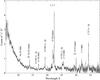 |
Fig. 1 The 2013−14 770 ks stacked RGS spectrum of NGC 5548 (observed frame). The strongest emission lines are labelled. The data points are shown in black. The data have been binned by a factor of two for clarity. |
3. Data analysis
Due to the low soft X-ray continuum flux, narrow emission lines (including He-like triplets of oxygen, nitrogen and neon) and radiative recombination continuum (RRC) features dominate the 2013−14 spectrum of NGC 5548. These features have not been seen so clearly in this source during previous observations, when the soft X-ray continuum was higher (e.g. Kaastra et al. 2000; Steenbrugge et al. 2003).
In order to accurately analyse the narrow emission features of this spectrum, a good model for the continuum and absorption was needed. Kaastra et al. (2014) conclude that the classical WA previously observed in NGC 5548 is not sufficient to explain the unexpected degree of absorption shown in this spectrum, and identify two new “obscurer” components needed to fit the intrinsic and reflected continuum well, in addition to six WA components (named from A to F; parameters shown in Table 1). The continuum was modelled with a combination of a modified black body and power-law, including reflection from distant material and an exponential cut-off at high energies. The details of this are in the supplementary materials of Kaastra et al. (2014). The exact physical interpretation of this continuum does not affect this work on the narrow emission features as it is used only as a continuum level above which we measure the emission features. Galactic neutral absorption is included with H I column density in the line of sight set to NH = 1.45 × 1020 cm-2 (Wakker et al. 2011). This continuum and absorption model is used throughout the analysis in this paper.
Due to low numbers of counts per bin, χ2 is not the appropriate goodness-of-fit parameter. Instead, goodness-of-fit should be measured by minimising the C-statistic (Cash 1979) parameter as it is based on the Poisson distribution and so does not suffer from the same drawbacks when using low count statistics. We therefore use the C-statistic for all analysis in this work. The errors used in this paper are all at the 1σ (68%) confidence level unless stated otherwise.
The high spectral resolution of RGS (λ/ Δλ ~ 340 at 22 Å; den Herder et al. 2001) compared to lower resolution X-ray spectroscopy leads to more detailed models being needed to fully describe the data. Our knowledge of many aspects of these models is not yet complete (for example presence of additional astrophysical components in the line of sight towards the source and imperfect atomic data) and we also have to deal with imperfect instrumental calibration, systematic effects and statistical fluctuations, so there will necessarily be differences between the data and the best physical model that can be found. As discussed in Blustin et al. (2002), the use of goodness-of-fit statistics when modelling RGS data must be coupled with careful consideration of the physical meaning of the models, as physical self-consistency is more important than reaching a nominally “acceptable” goodness-of-fit value.
All the spectral fitting in this paper was done with the spex1 spectral fitting program (Kaastra et al. 1996) version 2.05.02. Additional analysis compares simulated photoionisation spectral models from Cloudy (version 13.03; Ferland et al. 2013) with the observational data (Sects. 4 and 4.1). The adopted cosmological parameters in our modelling are H0 = 70 km s-1 Mpc-1, ΩΛ = 0.70 and Ωm = 0.30.
Broad emission line parameters from the 2013−14 RGS spectra.
Initial parameters for the O VII triplet from the 770 ks spectrum.
3.1. Broad emission lines
Although broad emission lines are difficult to identify in the 2013−14 spectrum, Kaastra et al. (2014) include four of these in their model (C VI Ly-α, O VII He-α, O VII He-β, O VIII Ly-α). All of their parameters (FWHM, luminosity and outflow velocity) were initially taken from the Steenbrugge et al. (2005) analysis of the Chandra LETGS 2002 spectrum, when the continuum was higher, and we begin by setting the broad lines at those values, using a Gaussian model for each. The 2002 parameters were estimated from knowledge of the UV broad line parameters in this source as they could not be directly fitted. We then allowed these parameters (FWHM, outflow velocity and luminosity of each line) to vary so we could fit them to the 2013−14 770 ks spectrum where possible (see Table 3). We take the broad line source to be interior to the obscurer, as expected from the results of Kaastra et al. (2014), therefore (as the fitted model parameters are different to the 2002 analysis) the new luminosities differ from those found previously. We can fit the broad O VIII Ly-α line (over the range 18.5−20 Å; C-stat = 80, and d.o.f. = 41) and the broad C VI Ly-α line (33.5−35 Å; C-stat = 75, and d.o.f. = 44), both shown in Fig. 2.
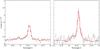 |
Fig. 2 The two broad emission lines that are well fitted; O VIII Ly-α (18.5−20 Å) and C VI Ly-α (33.5−35 Å). Both can be seen on the blue side of their corresponding narrow emission line. See text for details. |
For both of the O VII broad lines (He-α and He-β), we assume their FWHM and outflow velocity values have not changed since the values derived for the 2002 spectrum due to difficulties fitting new values in the 2013−14 spectrum. Therefore these two lines are set to their rest wavelength (i.e. assuming no outflow velocity), as they are in Steenbrugge et al. (2005). For the O VII He-α line this gives us a luminosity estimate, but for the O VII He-β this only gives an upper limit to the luminosity (see Table 3). As we only have an upper limit, we do not include the broad O VII He-β line in any further analysis.
The parameters for the O VIII Ly-α, O VII He-α and C VI Ly-α lines are fixed at the values in Table 3 throughout all the rest of the analysis in this paper.
3.2. Initial fit and He-like triplet diagnostics
There are He-like emission line triplets of oxygen, nitrogen and neon within the NGC 5548 stacked spectrum. The O VII triplet is the strongest and the O VII forbidden line component is the highest flux emission line in the data. For this reason, we have concentrated our diagnostics on the O VII triplet.
All three emission lines within any triplet (four if taking into account the intercombination line as an unresolved doublet) are expected to have consistent velocities. When fitting the He-like oxygen triplet by using three simple Gaussian models in spex, we found the forbidden and intercombination lines to have outflow velocities of −320 ± 40 km s-1 and −480 ± 160 km s-1 respectively, while the resonance line had a best fit velocity consistent with being at rest (−20 ± 50 km s-1; all values shown in Table 4).
First we looked at whether calibration issues could have caused this apparent difference by comparing with a 68 ks exposure of Capella taken close to our data, on 31-08-2013 (ObsID 0510781201), and processed the same way as our NGC 5548 data. We compared the line centroids of 8 strong emission lines between 6.64 and 33.74 Å with their laboratory wavelengths and found the weighted mean difference to be −2.7 ± 0.4 mÅ, corresponding to −17 ± 2 km s-1 at 20 Å. This very small offset is compatible with the typical orbital velocity of 30 km s-1 of the binary components of Capella, and shows that the uncertainties on the absolute wavelength scale are much smaller than the offsets we find for the forbidden and intercombination lines in our NGC 5548 data. In the Capella data, between 15 and 25 Å, the centroids of the five strongest lines were consistent within the error bars with the weighted mean and all had uncertainties of less than 30 km s-1. We conclude that there is no instrumental reason to doubt the measured line centroids of the O VII triplet in the NGC 5548 spectrum.
Further evidence that this velocity discrepancy is a real effect can be found in historical data; the same apparent velocity difference is seen in 1999 Chandra data, analysed by Kaastra et al. (2000, 2002), where the O VII resonance line appears ~300 km s-1 redshifted with respect to the O VII forbidden and intercombination lines, i.e. displaced in the same direction as we find in the 2013−14 spectrum. This previous work focussed on the narrow absorption lines that could be seen in the data, therefore those authors did not investigate the velocity discrepancy between these emission lines.
3.3. Investigation into O VII triplet velocity discrepancy
After ruling out calibration effects, we investigated various scenarios to explain the velocity discrepancy between the O VII triplet lines. First we explored the case in which we may be observing the combined emission from two ionised cones propagating out from the central source in opposite directions. Then we investigated the possibility that the velocity discrepancy is due to absorption.
3.3.1. Two cone model
First we looked at the possibility that the velocity discrepancy between the O VII triplet lines is caused by the presence of two contributing O VII triplets of different line ratios, one redshifted and one blueshifted with respect to the host galaxy. This could be the case if the narrow emission lines are being produced in two opposing cone shaped regions, each illuminated by and expanding away from the central source, with more gas in the cone closer to (and outflowing towards) the observer. In this case, the optically thin lines (such as forbidden and intercombination lines) would be seen from all of the gas and therefore would have one average (measured) velocity, dominated by that of the closer region with more gas. If the optically thick lines (such as the resonance line) are mainly produced at the illuminated face of the gas and shielded by the cooler gas, then we would preferentially see the lines formed in the gas which faces towards the observer (the further cone from us, outflowing away from us, and therefore redshifted). This would cause an apparent velocity difference between the resonance and both the intercombination and forbidden lines.
We tested this theory in spex by modelling each narrow emission line as a combination of two separate Gaussian components, one blueshifted and one redshifted, to represent the two opposing conical regions. The velocity difference between these components must be small enough that the observed emission lines retain their single peak appearance; this restriction is more important at longer wavelengths. The narrow emission line we observe in our data with the longest rest wavelength is C VI 1s-2p (33.736 Å), therefore the single peak appearance of this line in our data sets a limit on the velocity difference between the two conical regions in this model.
The best fit to the C VI 1s-2p line had ouflow velocities of −305 ± 40 and +125 ± 50 km s-1 for the blueshifted and redshifted components respectively. This model (with the outflow velocities fixed to those values) was then extended to fit all the emission lines in the spectrum, one by one, leaving widths and normalisations free. Finally the outflow velocities of the Gaussian components were left free to vary to find the final best fit for this model. The final best fit outflow velocities in this case are −320 ± 30 and + 190 ± 30 km s-1 respectively, with a C-statistic of 1832 (d.o.f. = 1027).
This model is not without problems, as the statistical best fit does not physically match the two cone model explained above. In this model the observed O VII forbidden line should be a combination of O VII forbidden emission from both the blueshifted and redshifted emission cones (as it is an optically thin line), whereas in the best fit model described above, the O VII forbidden line only has a contribution from the blueshifted Gaussian component (see Fig. 3). In contrast, the Ne IX and N VI forbidden lines in this model do have contributions from both the blue- and redshifted components, as expected. As we discuss in Sect. 3, physical self-consistency of our best fit model is the most important factor for acceptance, so for this reason we do not favour the two emission cone model as a physical explanation of the apparent O VII velocity discrepancy.
For completeness, we do look into this scenario further in Sect. 4.1 when investigating possible geometries for the narrow-line emitting gas using self-consistent photoionization models from Cloudy (this is not tried with spex as it does not yet include photoionisation emission models).
 |
Fig. 3 Final two cone model fit of the O VII triplet. Each emission line is fitted with two Gaussian components, one at velocity of −320 km s-1 (shown in blue) and the other at velocity of + 190 km s-1 (shown in red). The data are shown in black and the overall fit is shown in green. Clearly, the O VII forbidden line (on the right) only requires the blueshifted Gaussian component but this does not match the physical requirements of the two cone model (see text for details). |
3.3.2. Absorption
We then explored the possibility that the shift in the resonance line with respect to the other components of the O VII triplet is due to absorption on its blue side. This could then allow the true velocity of the resonance line to match the outflow velocity of around −300 km s-1 measured for the intercombination and forbidden lines. The resonance line could be more strongly affected by absorption than the other components of the triplet due to resonant scattering and the possible geometry of the region (Porquet et al. 2010). The comparative widths of these three lines, when simply fitted with Gaussian models, are already an indication that absorption may be playing a role in the appearance of the resonance line. As shown in Table 4, the measured width of the O VII resonance line is extremely small, especially compared to the intercombination and forbidden lines within that same O VII triplet. As all three of these lines should have the same widths, this implies that part of the resonance line is not being observed for some reason; absorption could cause this effect.
C-statistic values for fitting the O VII triplet, and the whole RGS spectrum, with WA absorption of narrow emission lines (and RRCs when looking at the whole data range).
We tested whether absorption of the triplet by any of the six WA components applied by Kaastra et al. (2014) could explain the shift of the resonance line in this way, as all WA components are found to have blueshifted velocities. Previous distance estimates for both the X-ray WA components (at least one component <7 pc; Detmers et al. 2008) and X-ray NLR (1−15 pc; Detmers et al. 2009) are similar, but the “obscurer” components discovered by Kaastra et al. (2014) are known to be located much closer to the ionising source than the NLR. Therefore these “obscurer” components were not included in this absorption test. Parameters of the WA components can be seen in Table 1. For this test the normalisations of the three O VII triplet lines were left free to vary after being placed inside each of the WA components in turn. The FWHM values for each of the O VII triplet lines were coupled and left free to vary. The outflow velocities for the three O VII triplet lines were also coupled and initially fixed to −300 km s-1 (the approximate outflow velocity of the forbidden line), to reduce the number of free parameters at this stage. This led to the C-statistic listed in Table 5. The outflow velocity is left free to vary after this test.
When comparing different, non-nested best fit models with the same number of degrees of freedom, as in this case, standard tests (such as the F-test) are not applicable, so we must use another method to determine if any improvement in the C-statistic is significant. In this case, given the tight relation between χ2 and C-statistic, we test the significance by taking the square root of the Δ C-statistic (measuring the improvement in C-statistic when comparing one model to another) and this gives us the significance of that improvement in σ. For example, ΔC of 9 corresponds to a 3σ improvement.
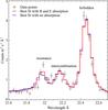 |
Fig. 4 Best fit model to O VII triplet. The data are shown in black. Shown in red is the best fit including absorption from X-ray WA components B and E (C-statistic = 82, for 43 d.o.f). Shown in blue is the best fit with no absorption (C-statistic = 104, for 43 d.o.f). In both models the outflow velocities and line widths of all three triplet lines are coupled together. The outflow velocity, line width and normalisations were left free to vary to find the best fit for each scenario. |
Narrow emission line best fit parameters from the 770 ks spectrum when absorption from WA components B and E is applied.
We focus on the results using only the O VII triplet wavelength range, as the C-stat of this region is not affected by any other regions where the continuum model does not match the data exactly (for example the excess of data over model in the range 35−38 Å). We conclude that one model is an improvement over another when the C-stat improves by ≥9, relating to a 3σ improvement.
As shown in Table 5 we also calculated the C-statistic values for each scenario over the whole spectrum. Initially we considered absorption by each WA component in turn; we determined that absorption by WA component B improved the fit substantially, and more so than the other components (from a C-stat of 104 to 93, d.o.f.=44). We then tested whether this fit further improved by adding another absorption component and found that including absorption by component E decreased the C-stat (by 10, to 83). Adding a third absorbing component (F) also decreased the C-stat around the triplet range again, but this time only by 5, so we do not consider this enough improvement to justify use of this model over the previous one. We also tested a different absorption scenario by using components A−C to absorb the narrow emission lines. This gave a better C-statistic when fit to the whole spectrum, but a worse value for only the O VII triplet range (see Table 5). As this test is focussed on how well we can fit the O VII triplet, we marginally prefer the scenario using absorption by B and E only because it requires a smaller number of absorbing components and gives a reasonable fit for both the O VII triplet and the whole spectrum.
We then allowed the outflow velocity of the triplet lines (still coupled together) to vary freely, using absorption from WA components B and E, giving a best fit outflow velocity of −300 ± 30 km s-1 (the C-statistic reduced by 1, to 82). This fit, compared to the fit with coupled O VII triplet line velocities but no absorption, is shown in Fig. 4. Clearly, the inclusion of absorption shifts the fitted peak of the O VII resonance line towards the peak seen in the data.
The evidence from these tests so far implies that WA components B and E are doing most of the absorbing of the O VII r line; we decided to explore how important the outflow velocities of these components are to this determination. To do this we took each of the other WA components and fixed their velocity to that of B and E in turn. Absorption by component A had very little effect on the fit around the O VII triplet, whether it was at its measured velocity or that of component B or E. We put this down to the fact that the measured velocities of components A, B and E are similar (−588 ± 34 km s-1, −547 ± 31 km s-1 and −792 ± 25 km s-1 respectively, taken from Kaastra et al. 2014). When the other components (C, D and F) were set to the velocities of components B and E, absorption by them caused a substantial improvement in the fit of the O VII triplet, compared to when they were set to their measured velocities. The C-statistic improved by between 5 and 29 (d.o.f. = 44) for each case.
The above indicates that having well determined outflow velocities for these warm absorber components is vital to calculate the effect that absorption by each one would have on the fit of the O VII triplet. Therefore the details of this absorption scenario for the narrow emission lines should be seen as strongly dependent on the determined warm absorber properties; in the context of this work we are testing the concept that the narrow emission lines could be absorbed by some warm absorber components, not the specific order of the involved warm absorber components.
While this absorption scenario does not give a perfect fit, it is the only physically plausible explanation for the O VII velocity discrepancy so far. Therefore we have used absorption by WA components B and E as our best fit scenario for the remainder of this work.
Using this absorption scenario for the O VII triplet, we recalculated the parameters of all narrow emission lines and RRCs (using the RRC model in spex, see Sect. 3.4.2) assuming that all are absorbed by the same combination of WA components. The results of this can be seen in Table 5. Absorbing all the narrow lines and RRCs by WA components B and E led to the best fit for the O VII triplet, but not for the whole spectrum. The best fit for the whole data range (5.7−38.2 Å) is obtained when the narrow lines and RRCs are all absorbed by WA components A, B and C; while this could be another physically acceptable scenario, the improved fit around the O VII triplet when absorbed by WA components B and E leads to our decision to focus on the latter for this work.
The best fit values for the narrow-line and RRC parameters over the whole spectrum, after absorption from WA components B and E, are presented in Sect. 3.4 and in Tables 6 and 7 respectively. These parameters are of course dependent on which scenario is used; here we adopt the simplest absorption scenario that gives the best fit to the O VII triplet region (with ΔC ≥ 9 from any simpler scenario).
3.4. spex best fit for the 770 ks stacked spectrum
3.4.1. Narrow emission line parameters
There are 14 narrow emission lines detected and an upper limit to one further narrow emission line in the stacked spectrum; their best-fit parameters are in Table 6. These were obtained using the absorption scenario (B and E absorption) described in detail in Sect. 3.3.2. We have checked all the best-fit values we would measure for parameters in Tables 6 and 7 if we had used absorption from WAs A−C (instead of B and E) and all are within 3σ uncertanties from the ones we provide. This shows that, for the X-ray narrow lines in this source, choosing a different specific absorption scenario does not significantly alter the overall results. The presence of this absorption is more important than which specific components are causing it.
Three complete emission triplets, of forbidden, intercombination and resonance lines (O VII, N VI and Ne IX) are present, plus four Ly-α (Ne X, N VII, O VIII and C VI), O VII He-α and O VIII Ly-β lines. These lines, with a few exceptions, were fitted using the simple Gaussian model in spex with the outflow velocity, FWHM and normalisation kept as free parameters. The exceptions to this are the Ne IX, O VII and N VI triplet lines, which had some values coupled together (see Table 6 for details), and the Ne X Ly-α and the Ne IX resonance and intercombination lines, which were fixed at their NGC 5548 rest frame wavelengths. The rest wavelengths were all taken from the internal spex line list.
Table 6 also shows which of these narrow lines have been previously detected in NGC 5548 (Kaastra et al. 2002; Steenbrugge et al. 2005; Detmers et al. 2009).
3.4.2. Radiative recombination continuum feature parameters
We detect eight RRC features in this spectrum; the final best fit parameters are presented in Table 7. All eight RRC features were simultaneously fitted with one RRC model in spex, which uses one temperature and allows different emission measures for each ion. This first RRC model gives an electron temperature in eV which is shown (along with the emission measures for each ion) in Table 7 (third column). The RRC features were then split into element pairs (e.g. O VII and O VIII together) and fitted with one RRC model for each pair. The carbon, oxygen and neon RRC models all give temperatures of the same order of magnitude (Table 7). The nitrogen RRC features are very weak in this spectrum, therefore the temperature for the nitrogen RRC model was fixed at the best fit value for that of the oxygen RRC model as the O VII RRC is the strongest, non-contaminated RRC feature in this spectrum. Nitrogen RRC emission measure values using this temperature are shown in Table 7. Fitting the RRC features in this “paired” way marginally improved the overall C-statistic by ΔC = 10 compared to using just one RRC model (and therefore one temperature) for all features. The best-fit temperatures for the carbon and neon RRC pairs are inconsistent with each other at the 3σ level (the uncertainties in Table 7 represent 1σ), which gives some evidence for stratification of the emission regions producing these RRC features.
The threshold energies (E) of all the RRC features are of the order of several hundred eV, and the electron temperatures (ΔE) are measured to be of the order of a few eV, therefore ΔE/E ≪ 1 which is strong evidence for photoionised conditions dominating within the emitting gas.
Results from automated fitting of the 770 ks stacked spectrum with Cloudy simulated spectra.
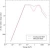 |
Fig. 5 The two SED shapes used as input for Cloudy. Cloudy scales the input SEDs using either luminosity or intensity values, so absolute values on the y-axis are not relevant. |
4. Testing the absorption model using Cloudy
In order to test the physical self-consistency of our modelling (as spex does not include a photoionised emission model) we use the spectral synthesis program Cloudy (Ferland et al. 2013). We created a number of simulated spectra for a range of physical parameters and compared them to our NGC 5548 data using the absorption scenario described above. We assume a plane parallel geometry, with the central source illuminating the inner face of the cloud and with a flux density dependent on a chosen ionisation parameter, ξ.
The spectrum produced by photoionisation processes strongly depends on the shape of the ionising continuum, described by the SED. Two sets of Cloudy results were compared with the 770 ks RGS spectrum; one was generated using the historical unobscured SED of NGC 5548 and one used the new obscured SED from 2013−14, both shown in Fig. 5. These SEDs are smoothed and simplified compared to those presented in Mehdipour et al. (2015a), but qualitatively very similar in shape, which is enough for this analysis. Both sets of Cloudy spectra were compared with the data in order to determine which gave the best fit. If the unobscured SED gives a better fit to the data, this would be evidence that we see the X-ray NLR as still receiving and reacting to the unobscured flux from the central source. If the obscured SED gives a better fit, then this would suggest that the NLR is located close enough to the central source that we see it as already receiving and reacting to the obscured flux.
For both SEDs, the Cloudy simulated spectra explored a parameter range of log ξ = 0.1−3.3 (with 0.2 step size), hydrogen column density =1021−1024 cm-2 (with 100.25 step size) and turbulent velocity = 101−103.5 km s-1 (with 100.5 step size). The electron density was set to 108 cm-3 because as long as this remains under the critical density2 for the species of interest (109−1010 cm-3; see Porquet & Dubau 2000; and Porter & Ferland 2007 for details) its value is unconstrained by the data we are comparing to.
The 1326 simulated spectra within this parameter grid for each SED were compared with the stacked 770 ks spectrum.
Each one of the Cloudy generated spectra was imported into a spex file model and compared with the data using an automated fitting process, with the normalisation of the simulated spectra left free to vary. This fitting process used a Python script to run spex and generate a C-statistic value for each one of the simulated spectra. Throughout this process there is no interpolation between the 1326 Cloudy models in the grid specified above. Unless otherwise stated, the Cloudy spectra were all given an outflow velocity of −300 km s-1 to match the measured value of the strongest emission line in the data, the O VII f line.
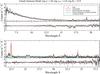 |
Fig. 6 Best fit self-consistent photoionisation model from Cloudy for all emission features (5.7−38.2 Å), including absorption from X-ray WA components B and E (see Kaastra et al. 2014 for details). C-statistic: 2273, d.o.f. = 1084. The data are shown in black, the best fit model is shown in red and the components of that model are shown in different colours and line styles. |
There are numerous possible outputs from Cloudy because, depending on the geometry of the system, the user may want to model emission in different directions. In terms of emission from the cloud, there are two directional components: reflected and transmitted. The reflected emission is from the illuminated face of the cloud (illuminated by the source), travelling back towards the source. The transmitted emission is the emission from the shielded face of the cloud and travels outwards (away from the source).
For this first test we chose to use the reflected spectrum output to model the narrow emission lines (as done in e.g. Bianchi et al. 2010; Guainazzi et al. 2009). This is of course only one potential geometry of the NLR region; more geometrical possibilities are explored in Sect. 4.1.
Each Cloudy reflected spectrum includes diffuse emission from within the cloud and scattered (absorbed and re-emitted) radiation from the intrinsic continuum, therefore it includes only the narrow emission lines and a scattered continuum. This means the incident continuum itself, WAs, obscurer and broad emission lines must be modelled separately. The observed continuum, WAs and obscurer are modelled as in Kaastra et al. (2014) and the 2013−14 broad emission line parameters from Sect. 3.1 in this paper are used. We tested whether the continuum should be left free to vary to allow any extra flux from the scattered Cloudy continuum to be included in the model without duplicating flux, but this did not change the results. There is not enough scattered continuum in the Cloudy spectra for this to be an important factor in the RGS band.
The narrow emission lines Cloudy produces are intrinsically narrower than those we see in the RGS data because, while Cloudy takes the effect of turbulence within the gas into account for the line strengths, it does not use this to broaden the lines in the produced spectra3. Therefore for the absorption to be applied properly, the narrow emission lines in the Cloudy spectra must be broadened. This was done using the vgau model in spex, set to a sigma velocity of 450 km s-1 as this was manually found to be the best overall fit to the data; it is also consistent with the average Gaussian sigma broadening value (460 ± 30 km s-1) found for all the narrow emission lines in Kaastra et al. (2014) and overall with the FWHM values in Table 6.
When fitting the whole 770 ks spectrum, we found that, with absorption from WA components B and E applied, the Cloudy results based on the obscured and unobscured SEDs gave best C-statistic values of 2213 and 2298 respectively (d.o.f. = 1084). All the C-statistic values from the Cloudy fits are collected in Table 8.
At this point we compared how well the Cloudy models from obscured and unobscured SEDs fit the data. In the RGS data range the Cloudy simulated spectra using the obscured SED gave a better fit to the data (ΔC = ~ 90). We tested to see if this is compatible with the rest of the NGC 5548 spectrum extending to the hard X-rays by applying our best fit model for the RGS band to the EPIC-pn data from the same campaign (see M. Cappi, in prep. for details of the analysis of the EPIC-pn data). This showed a severe excess of flux in the higher energy (>2 keV) range of the obscured SED Cloudy model in comparison to the EPIC-pn spectrum, and leads us to conclude that the Cloudy results from the unobscured SED are more physically appropriate, despite the slightly worse statistical quality of the fit in the RGS band.
In order to derive the errors in the best fit parameters for the emitting gas we created a finer grid of models with Cloudy, using the unobscured SED.
From this we calculate uncertainties on the parameters of the emitting gas for both absorption scenarios investigated above (B, E and A−C), giving 1σ uncertainties of log ξ = 1.45 ± 0.05, log NH = 22.9 ± 0.4 cm-2 and log vturb = 2.25 ± 0.5 km s-1. It is clear that the ionisation parameter of the emitting gas is much better constrained than the column density (and by extension the turbulent velocity, as this depends strongly on the column density).
This model is plotted in Fig. 6.
4.1. Testing further geometries with Cloudy
In the previous section we have investigated fitting the 770 ks spectrum with the reflected output from Cloudy models. As stated above, this is only one geometrical possibility for the NLR region, and so here we look into other potential geometries using different Cloudy outputs4.
In Sect. 4 we briefly described the outputs that Cloudy calculates are produced in different directions from the modelled cloud. The main transmitted (away from the source) output from Cloudy contains both the emission from the cloud itself and the attenuated emission from the source; for this work we do not want to include the attenuated emission from the source, so we additively combine the more specific Cloudy outputs of transmitted line emission and diffuse emission from the cloud. This approximates the outwards emission from the cloud without including the transmitted attenuated continuum emission, which is not appropriate as we are only using Cloudy to model the narrow emission lines, not all components of the total spectrum.
We compare three main different geometries to draw some simple conclusions; this is by no means a full investigation into all possible geometries of this system. These tests were all done with the Cloudy grid of models used in the previous section, but with varying outputs used.
Geometry 1) The simplest interpretation of the reflected output, adopted in the previous section, is that we are observing emission from the illuminated face of NLR clouds on the opposite side of the source to our line of sight.
Geometry 2) We could be observing emission from the shielded face of NLR clouds on the same side of the source as our line of sight. The Cloudy outputs of transmitted lines and diffuse emission were additively combined to approximate this geometry. The best fit parameters for this geometry gave a C-stat value of ~300 larger than the best fit for geometry 1), with smaller NH, but very similar ξ and vturb values (log ξ = 1.5, log NH = 22 and log vturb = 2.5).
Geometry 3) We could be observing a combination of the two above geometries: emission from both the illuminated face of NLR clouds on the far side of the source and the shielded face of NLR clouds on the near side of the source, with respect to our line of sight. To model this we used a combination of the outputs used for geometries 1) and 2) above. To restrict the permutations of this geometry, and therefore reduce computational time, we made the simplifying assumption that both the near and far NLR clouds have the same parameters (ξ, NH and vturb). The reflected output (representing emission from clouds on the far side of the source) was given a positive velocity shift (+300 km s-1) and the transmitted outputs (representing emission from clouds on the near side of the source) were given a negative velocity shift of (−300 km s-1), so that both are outflowing away from the source. We tested this geometry in three ways: i) with no absorption of either emission components; ii) with absorption of the far clouds’ emission (the reflected output) by WA components B and E and no absorption of the near clouds’ emission; and iii) with absorption of the far clouds’ emission (the reflected output) by all WA components (A−F) and no absorption of the near clouds’ emission. The first form of this geometry, i), also represents the two-cone scenario we discussed in Sect. 3.3.1; while our previous tests using spex indicated this geometry is not applicable to NGC 5548, we have included it here for completeness within our Cloudy tests. In all three cases, i)−iii), the best fit parameters were: log ξ= 1.5, log NH = 22.25 and log vturb = 2.5. The best of these cases, in terms of C-statistic value, is ii), but even in this case the C-statistic value is ~200 larger (d.o.f. = 1083) than the best fit for geometry 1).
These tests have shown that, when comparing these three simple geometries, emission from the illuminated face of the cloud modelled in Cloudy is the best match to the narrow emission line data of NGC 5548. The simplest interpretation is that the NLR we see is emission from the illuminated face of clouds on the far side of the source. Assuming there are absorbing clouds (WAs) closer to the source than the NLR (or on the near side of the source), then absorption of the NLR emission by these clouds would explain the velocity discrepancy seen in the O VII triplet (see Sect. 3.3.2). The problem with this interpretation is that these emission lines are blueshifted, therefore if this emission was coming from the far side of the source the emitting material would be inflowing towards the source, not outflowing from it, as we would expect.
It is very likely that the geometry in this system is more complex than the plane-parallel cloud assumed in Cloudy to cause this, so we cannot be more specific at this stage.
5. Discussion
As previously stated, the 2013−14 770 ks RGS spectrum shows the largest number of soft X-ray narrow emission lines and RRC features ever observed in NGC 5548. In total, fourteen narrow lines and eight RRCs are detected, with upper limits for one more narrow emission line. Due to the low soft X-ray continuum flux during these observations, we identify six narrow lines and six RRCs which had not previously been detected in NGC 5548. We also present new parameters for eight narrow emission lines and two RRCs identified in previous observations of this source.
We detect six of the ten narrow lines found by Steenbrugge et al. (2005); one of their lines (C V f) falls outside our wavelength range, and the other three (Mg XI f, Al XII f and Si XIII f) are in the steep, noisy short wavelength part of our spectrum, so it is very difficult to set stringent limits to their parameters using these data.
Using photoionisation models from Cloudy we have constrained the emitting gas to an ionisation parameter of log ξ = 1.45 ± 0.05, column density of log NH = 22.9 ± 0.4 cm-2 and turbulent velocity of log vturb = 2.25 ± 0.5 km s-1. Using the same conversion between the ionisation parameters of ξ and U as in Arav et al. (2015) for the historical SED of NGC 5548 (log ξ = log U + 1.6), we gain an estimate for our emitting gas of log U = −0.15 ± 0.05. We can now compare both the ionisation parameter and column density from this work to similar work on other Seyfert objects (see Table 2 for a summary of previous work). The column density value we find (1022.9 ± 0.4 cm-2) is similar to the highest values found for other objects. For example NGC 4051, NGC 4151 and NGC 1365 (by Nucita et al. 2010; Armentrout et al. 2007; Guainazzi et al. 2009, respectively) are all found to need emitting gas with column densities of the order of 1023 cm-2 in order to model their X-ray NLR emission. Our NGC 5548 ionisation parameter, converted to log U = −0.15 ± 0.05, is lower than most for other Seyfert galaxies, except for the low ionisation component of the three phase model for NGC 4151 (Armentrout et al. 2007). As expected, our ionisation parameter is higher than that needed to model the UV narrow emission lines in NGC 5548 itself (Kraemer et al. 1998). Due to the much higher soft X-ray continuum flux in previous observations of NGC 5548, and therefore a much smaller number of measurable X-ray narrow emission lines, this is the first time photoionisation modelling has been used to constrain the ionisation parameter and column density of the X-ray narrow-line emitting gas in this galaxy.
5.1. Warm absorption of the NLR
Our initial fit (using a Gaussian model in spex for each narrow line) to the 2013−14 stacked spectrum of 770 ks shows a difference in velocity between the O VII resonance line (−20 ± 50 km s-1) and the forbidden and intercombination lines (−320 ± 40 km s-1 and −480 ± 160 km s-1, respectively). This result is hard to interpret physically; the triplet lines should all be formed by the same plasma and therefore have consistent velocities. We investigated possible explanations for this mismatch of velocities such as calibration effects, emission from two ionisation cones, and absorption, concluding that absorption is most likely (as detailed in Sect. 3.3).
An alternative hypothesis could be considered, that the O VII triplet may be a superposition of emission by photoionised and collisional plasmas, such as found in star forming regions. However, this is very unlikely; NGC 5548 does not have a high star formation rate, and the AGN is too bright to allow any star formation rate contribution to be detected unless it were a very significant one (Doroshenko et al. 1998).
Our main result, which resolves the velocity discrepancy of the O VII triplet, is by having the narrow emission lines absorbed by at least one of the six X-ray WA components found by Kaastra et al. (2014). The implications of this in terms of the distance of the NLR from the source are discussed in Sect. 5.3 below.
A similar result has been obtained for the UV narrow emission lines in NGC 7469, where Kriss et al. (2003) found that the best fit to their Far Ultraviolet Spectroscopic Explorer (FUSE) data included absorption of the narrow emission line components by the UV warm absorbers, at the same covering fraction as the absorption of the broad emission lines and continuum.
Using the best fit model from the scenario with absorption of both the narrow emission lines and RRC features by WA components B and E, we calculated the ratio of the unabsorbed flux of O VII RRC to the O VII forbidden line (RRC/f), as was done in Kaastra et al. (2002). The 2013−14 absorption scenario RRC/f value is 0.44 ± 0.05, much closer to (and consistent within 3σ to) the value of 0.57 from Behar et al. (2002) photoionisation models for an adopted temperature of 5 eV 5 than the value from the 1999 observations (0.07 ± 0.12; Kaastra et al. 2002). Within Kaastra et al. (2002) the authors suggest that their smaller than expected RRC/f value may be due to a combination of limited statistics and nearby WA absorption features contaminating the RRC flux measurement. Without WA absorption of either narrow emission lines or RRCs, a smaller than expected RRC/f value is also observed in the 2013−14 data (0.28 ± 0.03), which again is not at all consistent with the model value. Therefore including the absorption by WA components B and E of both the RRCs and the narrow emission lines greatly reduces the tension between observed and modelled O VII RRC/f values, further supporting this absorption scenario.
5.2. NLR reacting to unobscured SED
Our work using Cloudy (see Sect. 4), with both RGS and EPIC data, shows that the narrow-line emitting gas is still reacting to the unobscured SED. This implies that we should not expect any additional variation in the narrow lines compared to previous observations and levels of variability between them. As previous analysis of historical observations did not take into account any absorption of the narrow lines by the WAs that we now see, in order to make appropriate comparisons we must make the same assumptions as in previous analyses. The 2013−14 O VII f unabsorbed flux, calculated without including any absorption by WA components, is 0.65 photons m-2 s-1, which is between values from observations between 1999 and 2001 (4 observations, with flux values 0.81 ± 0.16, 0.82 ± 0.18, 1.3 ± 0.2 and 1.1 ± 0.1 photons m-2 s-1, in chronological order), and the 2005 and 2007 values (0.35 ± 0.06 and 0.27 ± 0.06 photons m-2 s-1 respectively), when the source was seen in an unobscured but intrinsically low-flux state (these historical measurements of O VII f fluxes are collated in Detmers et al. 2009). The unabsorbed flux of the O VII f line in 2002 (0.75 ± 0.07 photons m-2 s-1) is the historical value closest to our 2013−14 measurement, still differing from it by just over the 1σ level. We conclude that there is marginal evidence for variability between 2013−14 and some previous epochs, which is well within the expected range for this source (Detmers et al. 2009). This supports our claim that the NLR is still reacting to the unobscured SED, as it would have been during all these previous epochs.
5.3. Distance estimates of NGC 5548’s X-ray NLR
In our best fit absorption scenario, the emitting gas (determined from Cloudy modelling) has the parameters: log ξ = 1.45 ± 0.05, log NH = 22.9 ± 0.4 and log vturb = 2.25 ± 0.5. Using this result, and the definition of ξ (ξ ≡ L/nr2, Sect. 1) we can determine a lower limit to the distance of the emitting gas from the source. We use n< 5 × 109 cm-3 as this is the critical density for O VII (Porquet & Dubau 2000) and as we know this gas is photoionised (from the presence of narrow RRCs), the density must be below this value. L (= 11.7 × 1043 erg s-1) is taken from Mehdipour et al. (2015a), and is the luminosity of the unobscured 2013−14 SED, and ξ (log ξ = 1.45) is taken from the Cloudy best fit to the data. This gives a (not very restrictive) lower limit to the distance of the emitting gas of r> 9.3 × 10⁻³ pc.
For another distance estimate, we can begin by writing the column density, NH, as: 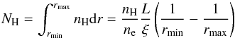 (1)which, using the same method as Behar et al. (2003) and assuming rmax ≫ rmin, can be rewritten as:
 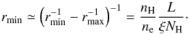 (2)We can then use the simplifying relation ne = 1.2nH (for a fully ionized cosmic plasma), and our values of L, ξ and NH (see previous paragraph) to calculate rmin = 13.9 ± 0.6 pc. This is consistent with the previous distance estimate of 1−15 pc for the X-ray NLR by Detmers et al. (2009), especially when considering that the Cloudy modelling in this work suggests that the narrow-line emission comes mainly from the illuminated face of the NLR cloud(s), which would be located at rmin.
We note that the log ξ value of the emitting gas found from Cloudy analysis, 1.45 ± 0.05, is consistent with the 2002 log ξ value of WA component B (1.51 ± 0.05, when the WAs were reacting to the unobscured ionizing flux). Combining this with the consistent distance estimates for the X-ray NLR (rmin = 13.9 ± 0.6 pc, this work; 1−15 pc, Detmers et al. 2009) and WA component B (<40 pc, J. Ebrero, in prep.), can we identify the NLR emission gas with the WA absorption gas? The column density for the emitting gas determined with Cloudy, log NH = 22.9 ± 0.4 cm-2, is higher than the combined column densities of all WA components. However, WAs are seen along the line of sight while the X-ray NLR emission is likely coming from a much larger region, given the fact that it is still reacting to the unobscured SED, so there could be column density variations over that region. The coincidence of ionisation parameters and compatible distances of the X-ray NLR gas with one of the WA components is not seen here as enough evidence to conclusively identify any of the WA components as the same physical gas as the narrow-line emitting gas, although it is suggestive of that possibility.
6. Conclusions
We have used the 770 ks RGS spectrum of NGC 5548 from our 2013−14 observational campaign to show evidence that the narrow emission lines undergo absorption by at least one of the six known warm absorber (WA) components in this source. There are indications that the main absorption comes from WA component B (labelled as such by Kaastra et al. 2014). We have established this from careful analysis of the O VII triplet, in the wavelength range 21.5−23 Å. This solution also resolves tension between modelled and observed values of the O VII RRC/f unabsorbed flux ratio. Unfortunately the data do not allow us to conclusively distinguish between competing detailed scenarios of absorption of the narrow emission lines by different combinations of WA components. The presence of this absorption is a more important result than which of the specific components are causing it.
Through comparison to simulated spectra produced by the photoionisation code Cloudy, we use both RGS and EPIC-pn data to determine that the emitting gas can be described as reacting to the unobscured SED (i.e. to ionising radiation before the intervention of the “obscurer” discovered in our observing campaign). The emitting gas has a well constrained ionisation parameter of log ξ = 1.45 ± 0.05 and column density and turbulent velocity of log NH = 22.9 ± 0.4 cm-2 and log vturb = 2.25 ± 0.5 km s-1 respectively. This is the first time the X-ray NLR emitting gas in this source has been characterised by an ionisation parameter and column density. From this we estimate the distance of these emitting clouds from the central source as 13.9 ± 0.6 pc.
The critical density for any species is the density at which collisional and radiative de-excitation rates are equal; collisional processes become more (less) important for higher (lower) densities.
See Hazy 1 documentation, page 162.
For detailed information of Cloudy’s geometry see Hazy 1, page 6.
As the temperature dependence of this ratio is weak (Kaastra et al. 2002), and our best fit temperature from the pair of oxygen RRCs (O VII and O VIII) is 6.6 ± 0.06 eV, this is a reasonable comparison to make.
Acknowledgments
The data used in this research are stored in the public archives of the satellites that are involved. We thank the International Space Science Institute (ISSI) in Bern for support. This work is based on observations obtained with XMM-Newton, an ESA science mission with instruments and contributions directly funded by ESA Member States and the USA (NASA). M. W. acknowledges the support of a Ph.D. studentship awarded by the UK Science & Technology Facilities Council (STFC). SRON is supported financially by NWO, the Netherlands Organization for Scientific Research. M.M. acknowledges the support of a Studentship Enhancement Programme awarded by the UK Science & Technology Facilities Council (STFC). K.C.S. acknowledges financial support from the Fondo Fortalecimiento de la Productividad Científica VRIDT 2013. E.B. is supported by grants from Israel’s MoST, ISF (1163/10), and I-CORE program (1937/12). B.M.P. acknowledges support from the US NSF through grant AST-1008882. M.C. and S.B. acknowledge INAF/PICS support. G.P. acknowledges support via an EU Marie Curie Intra-European fellowship under contract no. FP-PEOPLE-2012-IEF-331095. P.O.P. acknowledges funding support from the CNES and the French-Italian International Project of Scientific Collaboration: PICS-INAF project n181542. This research has made use of the NASA/IPAC Extragalactic Database (NED), which is operated by the Jet Propulsion Laboratory, California Institute of Technology, under contract with the National Aeronautics and Space Administration. This research has made use of NASA’s Astrophysics Data System Bibliographic Services’. M.W. thanks Mat Page for useful discussions. The authors thank the anonymous referee for the useful suggestions.
References
- Arav, N., Chamberlain, C., Kriss, G. A., et al. 2015, A&A, 577, A37 [NASA ADS] [CrossRef] [EDP Sciences] [Google Scholar]
- Armentrout, B. K., Kraemer, S. B., & Turner, T. J. 2007, ApJ, 665, 237 [NASA ADS] [CrossRef] [Google Scholar]
- Behar, E., Kinkhabwala, A., Sako, M., et al. 2002, Mass Outflow in Active Galactic Nuclei: New Perspectives, ASP Conf. Proc., 255, 43 [NASA ADS] [Google Scholar]
- Behar, E., Rasmussen, A. P., Blustin, A. J., et al. 2003, ApJ, 598, 232 [NASA ADS] [CrossRef] [Google Scholar]
- Bentz, M. C., Walsh, J. L., Barth, A. J., et al. 2009, ApJ, 705, 199 [NASA ADS] [CrossRef] [Google Scholar]
- Bianchi, S., Guainazzi, M., & Chiaberge, M. 2006, A&A, 448, 499 [NASA ADS] [CrossRef] [EDP Sciences] [Google Scholar]
- Bianchi, S., Chiaberge, M., Evans, D. A., et al. 2010, MNRAS, 405, 553 [NASA ADS] [Google Scholar]
- Blustin, A. J., Branduardi-Raymont, G., Behar, E., et al. 2002, A&A, 392, 453 [NASA ADS] [CrossRef] [EDP Sciences] [Google Scholar]
- Cash, W. 1979, ApJ, 228, 939 [NASA ADS] [CrossRef] [Google Scholar]
- Chiang, J., Reynolds, C. S., Blaes, O. M., et al. 2000, ApJ, 528, 292 [NASA ADS] [CrossRef] [Google Scholar]
- de Vaucouleurs, G., de Vaucouleurs, A., Corwin, Jr., H. G., et al. 1991, Third Reference Catalogue of Bright Galaxies, Vol. I: Explanations and references, Vol. II: Data for galaxies between 0h and 12h, Vol. III: Data for galaxies between 12h and 24h (Springer, New York, USA) [Google Scholar]
- den Herder, J. W., Brinkman, A. C., Kahn, S. M., et al. 2001, A&A, 365, L7 [NASA ADS] [CrossRef] [EDP Sciences] [Google Scholar]
- Denney, K. D., De Rosa, G., Croxall, K., et al. 2014, ApJ, 796, 134 [NASA ADS] [CrossRef] [Google Scholar]
- Detmers, R. G., Kaastra, J. S., Costantini, E., McHardy, I. M., & Verbunt, F. 2008, A&A, 488, 67 [NASA ADS] [CrossRef] [EDP Sciences] [Google Scholar]
- Detmers, R. G., Kaastra, J. S., & McHardy, I. M. 2009, A&A, 504, 409 [NASA ADS] [CrossRef] [EDP Sciences] [Google Scholar]
- Doroshenko, V. T., Lyutyi, V. M., & Shenavrin, V. I. 1998, Astron. Lett., 24, 160 [NASA ADS] [Google Scholar]
- Erkens, U., Appenzeller, I., & Wagner, S. 1997, A&A, 323, 707 [NASA ADS] [Google Scholar]
- Ferland, G. J., Porter, R. L., van Hoof, P. A. M., et al. 2013, Rev. Mex. Astron. Astrofis. 49, 137 [Google Scholar]
- Guainazzi, M., Risaliti, G., Nucita, A., et al. 2009, A&A, 505, 589 [NASA ADS] [CrossRef] [EDP Sciences] [Google Scholar]
- Kaastra, J. S., Mewe, R., & Nieuwenhuijzen, H. 1996, 11th Colloq. UV and X-ray Spectroscopy of Astrophysical and Laboratory Plasmas, 411 [Google Scholar]
- Kaastra, J. S., Mewe, R., Liedahl, D. A., & Brinkman, A. C. 2000, A&A, L83 [Google Scholar]
- Kaastra, J. S., Steenbrugge, K. C., Raassen, A. J. J., et al. 2002, A&A, 386, 427 [NASA ADS] [CrossRef] [EDP Sciences] [Google Scholar]
- Kaastra, J. S., de Vries, C. P., Steenbrugge, K. C., et al. 2011, A&A, 534, A37 [NASA ADS] [CrossRef] [EDP Sciences] [Google Scholar]
- Kaastra, J. S., Kriss, G. A., Cappi, M., et al. 2014, Science, 345, 64 [NASA ADS] [CrossRef] [Google Scholar]
- Kinkhabwala, A., Sako, M., Behar, E., et al. 2002, ApJ, 575, 732 [NASA ADS] [CrossRef] [Google Scholar]
- Korista, K. T., Alloin, D., Barr, P., et al. 1995, ApJS, 97, 285 [NASA ADS] [CrossRef] [Google Scholar]
- Kraemer, S. B., Crenshaw, D. M., Filippenko, A. V., & Peterson, B. M. 1998, ApJ, 499, 719 [NASA ADS] [CrossRef] [Google Scholar]
- Kriss, G. A., Blustin, A., Branduardi-Raymont, G., et al. 2003, A&A, 403, 473 [NASA ADS] [CrossRef] [EDP Sciences] [Google Scholar]
- Longinotti, A. L., Nucita, A., Santos-Lleo, M., & Guainazzi, M. 2008, A&A, 484, 311 [NASA ADS] [CrossRef] [EDP Sciences] [Google Scholar]
- Marinucci, A., Bianchi, S., Matt, G., et al. 2010, A&A, 526, A36 [Google Scholar]
- Mehdipour, M., Kaastra, J. S., Kriss, G. A., et al. 2015a, A&A, 575, A22 [NASA ADS] [CrossRef] [EDP Sciences] [Google Scholar]
- Mehdipour, M., Kaastra, J. S., & Raassen, A. J. J. 2015b, A&A, 579, A87 [NASA ADS] [CrossRef] [EDP Sciences] [Google Scholar]
- Nucita, A. A., Guainazzi, M., Longinotti, A. L., et al. 2010, A&A, 515, A47 [NASA ADS] [CrossRef] [EDP Sciences] [Google Scholar]
- Peterson, B. M., Berlind, P., Bertram, R., et al. 2002, ApJ, 581, 197 [NASA ADS] [CrossRef] [Google Scholar]
- Peterson, B. M., Ferrarese, L., Gilbert, K. M., et al. 2004, ApJ, 613, 682 [NASA ADS] [CrossRef] [Google Scholar]
- Peterson, B. M., Denney, K. D., De Rosa, G., et al. 2013, ApJ, 779, 109 [NASA ADS] [CrossRef] [Google Scholar]
- Porquet, D., & Dubau, J. 2000, A&AS, 143, 495 [NASA ADS] [CrossRef] [EDP Sciences] [Google Scholar]
- Porquet, D., Dubau, J., & Grosso, N. 2010, Space Sci. Rev., 157, 103 [NASA ADS] [CrossRef] [Google Scholar]
- Porter, R. L., & Ferland, G. J. 2007, ApJ, 664, 586 [NASA ADS] [CrossRef] [Google Scholar]
- Rodríguez-Ardila, A., Viegas, S. M., Pastoriza, M. G., & Prato, L. 2002, ApJ, 579, 214 [NASA ADS] [CrossRef] [Google Scholar]
- Steenbrugge, K. C., Kaastra, J. S., de Vries, C. P., & Edelson, R. 2003, A&A, 402, 477 [NASA ADS] [CrossRef] [EDP Sciences] [Google Scholar]
- Steenbrugge, K. C., Kaastra, J. S., Crenshaw, D. M., et al. 2005, A&A, 434, 569 [NASA ADS] [CrossRef] [EDP Sciences] [Google Scholar]
- Tarter, C. B., Tucker, W. H., & Salpeter, E. E. 1969, ApJ, 156, 943 [NASA ADS] [CrossRef] [Google Scholar]
- Wakker, B. P., Lockman, F. J., & Brown, J. M. 2011, ApJ, 728, 159 [NASA ADS] [CrossRef] [Google Scholar]
All Tables
Parameters of the 2013−14 warm absorber components (WA comp.) from Kaastra et al. (2014).
Previously reported results of Seyfert galaxy narrow line region modelling using Cloudy.
C-statistic values for fitting the O VII triplet, and the whole RGS spectrum, with WA absorption of narrow emission lines (and RRCs when looking at the whole data range).
Narrow emission line best fit parameters from the 770 ks spectrum when absorption from WA components B and E is applied.
Results from automated fitting of the 770 ks stacked spectrum with Cloudy simulated spectra.
All Figures
|
Fig. 1 The 2013−14 770 ks stacked RGS spectrum of NGC 5548 (observed frame). The strongest emission lines are labelled. The data points are shown in black. The data have been binned by a factor of two for clarity. |
| In the text | |
|
Fig. 2 The two broad emission lines that are well fitted; O VIII Ly-α (18.5−20 Å) and C VI Ly-α (33.5−35 Å). Both can be seen on the blue side of their corresponding narrow emission line. See text for details. |
| In the text | |
|
Fig. 3 Final two cone model fit of the O VII triplet. Each emission line is fitted with two Gaussian components, one at velocity of −320 km s-1 (shown in blue) and the other at velocity of + 190 km s-1 (shown in red). The data are shown in black and the overall fit is shown in green. Clearly, the O VII forbidden line (on the right) only requires the blueshifted Gaussian component but this does not match the physical requirements of the two cone model (see text for details). |
| In the text | |
|
Fig. 4 Best fit model to O VII triplet. The data are shown in black. Shown in red is the best fit including absorption from X-ray WA components B and E (C-statistic = 82, for 43 d.o.f). Shown in blue is the best fit with no absorption (C-statistic = 104, for 43 d.o.f). In both models the outflow velocities and line widths of all three triplet lines are coupled together. The outflow velocity, line width and normalisations were left free to vary to find the best fit for each scenario. |
| In the text | |
|
Fig. 5 The two SED shapes used as input for Cloudy. Cloudy scales the input SEDs using either luminosity or intensity values, so absolute values on the y-axis are not relevant. |
| In the text | |
|
Fig. 6 Best fit self-consistent photoionisation model from Cloudy for all emission features (5.7−38.2 Å), including absorption from X-ray WA components B and E (see Kaastra et al. 2014 for details). C-statistic: 2273, d.o.f. = 1084. The data are shown in black, the best fit model is shown in red and the components of that model are shown in different colours and line styles. |
| In the text | |
Current usage metrics show cumulative count of Article Views (full-text article views including HTML views, PDF and ePub downloads, according to the available data) and Abstracts Views on Vision4Press platform.
Data correspond to usage on the plateform after 2015. The current usage metrics is available 48-96 hours after online publication and is updated daily on week days.
Initial download of the metrics may take a while.